1. Introduction
Active matter provides a playground to study non-equilibrium statistical physics and self-organizing properties of living systems [
1,
2]. The constitutive ingredients are the active particles which, unlike in thermal equilibrium, constantly consume and dissipate energy to propel or perform mechanical work. Because a unifying description of these non-equilibrium systems is missing, it is important to explore the properties of simple models and their relation to equilibrium statistical physics.
Two classes of simple activity models can be determined. The prominent
vectorial class, where the particles are propelled in a given direction that randomizes through various mechanisms on longer time scales, includes Viscsek model, Active Brownian particles, Run and Thumble, and Ornstein–Uhlenbeck particles [
3,
4,
5,
6,
7]. The simpler and less explored
scalar activity, on which we focus in this work, is modeled as thermal-like fluctuations of elevated temperature with respect to the passive surroundings. Therefore, it is defined in mixtures of active and passive particles [
8,
9].
It was shown that a sufficiently high temperature ratio of the two particle species results in a phase separated steady state [
8,
9]. While the critical ratio is unfeasibly high for colloidal particles, if the particles are polymers, the ordered phase may be experimentally realized, as the critical ratio decreases with their length [
10]. This supports the hypothesis that the effect might play a role in separation of active and passive DNA strands in living cells [
9,
10,
11,
12]. There, the activity can originate from transcription, repair or looping extrusion processes that consume energy to fuel the molecular motors that drag the DNA strands. For example, it was observed that the euchromatin, the transcriptionally active DNA fiber, is spatially separated from the mostly transcriptionally silent heterochromatin. As shown in [
13], some data on the dynamics of the active DNA fibers in living cells can be understood by such a simple two-temperature model.
The heat transport and related entropy production both take place at the interface and govern the system’s behavior [
10]. Investigating the interface of the phase-separated steady state can help to reveal not only the underlying principles of the non-equilibrium phase transition, but also new phenomena. For example, there are indications that a spontaneously separated
vectorial active matter exhibits similar interfacial fluctuation spectra as the equilibrium phase separated state [
14,
15,
16]. However, unlike in equilibrium, positive interfacial stiffness arises as a competition between negative interfacial tension and the work of oriented active particles stabilizing the interface. These features are hypothesized to be a generic characteristic of activity induced phase separated matter, but it is not clear if this applies to scalar activity blends as well. Comparing the interfacial properties of the non-equilibrium steady states with equilibrium phase-separated systems enables delineation of where the physical understanding built on the equilibrium systems is applicable.
In this work, we use molecular dynamics (MD) to study the interfacial properties of a well-separated steady state of a blend of two identical polymer types connected to two different thermostats. First, we describe the model details. Subsequently, we characterize the interface profiles, derive the phase diagrams, explore the critical behavior, and show that the entropy production is an accurate indicator of the phase transition. A significant part of our study is dedicated to interface fluctuations. We characterize their spectrum, which allows for a mechanistic definition of the interfacial stiffness. The various results point to a common conclusion that this non-equilibrium system resembles in many respects an equilibrium polymer blend with a lower critical solution temperature.
Model
Our system consists of
M monodisperse fully flexible chains of
monomers with purely repulsive shifted Lennard–Jones interactions with a cutoff at
The chain connectivity is maintained by the finitely extensible nonlinear elastic (FENE) potential
where
and
The natural time scale of this standard polymer model is
. All energy quantities are in units of
and the Boltzmann constant is set to unity.
of the chains are coupled to a “cold” Langevin thermostat with temperature
and the other half to a “hot” Langevin thermostat of
. Each thermostat is coupled to the system by the same coupling friction
. In the original work on polymers, Ref. [
10]
was chosen to be rather high
to be comparable to the overdamped limit used in other works [
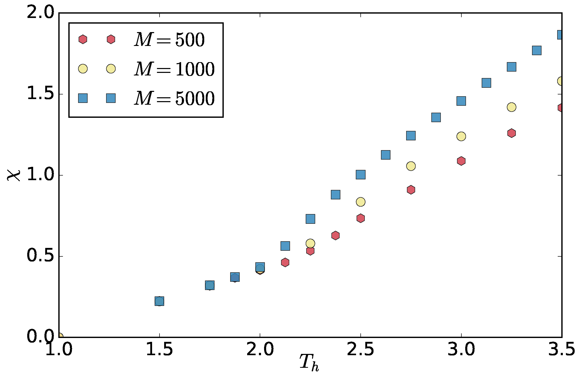
11] and to observe phase separation at relatively low thermostat temperatures. The critical temperature of the hot thermostat decreases with increasing friction (see
Figure 1a) because the heat transfer from the thermostat to the particles becomes more efficient, which increases the difference between the effective temperature of the hot and the cold particles. As mentioned in [
10], a natural asymmetry parameter of the system is
which captures the relative difference in the effective temperatures
and
(one third of the mean squared velocity) of the hot and cold components, respectively. We use
because of its low sensitivity to the choice of friction as shown in
Figure 1b, where we compare order parameter profiles for different frictions for the system of
chains. The order parameter used is
, where
x is the average inter-chain like-particles number fraction in a
neighborhood i.e., if inter-chain cold-cold monomer contacts are equally likely to hot-cold
. As can be seen in
Figure 1b, some systematic variation with
still remains, which we leave for future study.
To obtain a well separated state for profile and capillary wave analysis, we start with an equilibrium configuration of a well mixed system at a constant volume setting with density of , temperature with periodic boundary conditions. We connect the hot chains to the hot thermostat of , which is sufficient for phase separation to occur given the coupling friction used throughout this work. We simulate the system with time step until the phase separated steady state is reached. This process typically takes about the time needed for all the chains to diffuse through the whole system. Above the critical temperature ratio, the interface aligns with one of the box coordinates as is typical also for the equilibrium phase separation—there, due to the minimization of the interfacial area. For our largest system of , the aligned steady states were observed for at least . We sampled the configurations every , which is enough time to get uncorrelated chain conformations. We had at least 400 configurations for each in total.
To characterize the steady state, we will use various averages of the physical quantities. The brackets stand for average over the ensemble of the configurations in the steady state and this represents an average over subset of the phase space that characterizes the steady state. For certain quantities, such as the density, the average can vary with distance from the interface. In that case, the average at a given distance is calculated over the steady state configurations of the particles that fall within a given slab at that distance.
2. Profiles and Phase Diagrams of Density and Effective Temperature
The phase separation occurs because the local difference in temperatures gives rise to a pressure difference that is compensated with a density change by the redistribution of the particles. In steady state, the mass transport is suppressed, and heat flow is mostly localized at the interfaces. Therefore, in a separated steady state, the effective temperature and density exhibit non-constant profiles, while the pressure tensor component perpendicular to the interface is constant (hydrostatic equilibrium
). To investigate the profiles, we orient the interface perpendicular to the
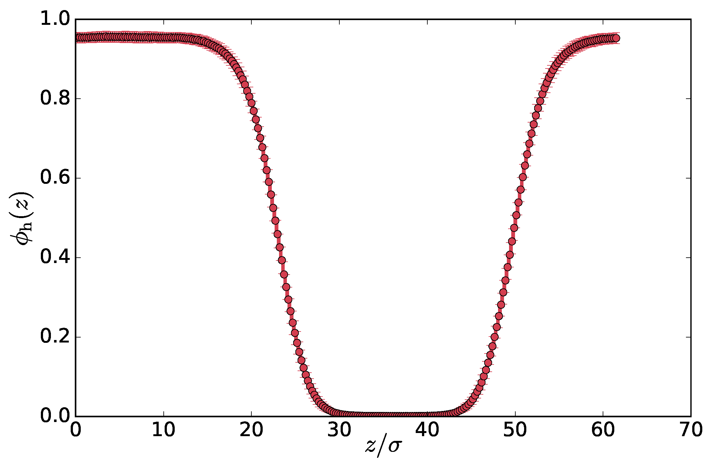
z-axis and align the different system snapshots by subtracting the center of mass from the coordinates. The average density exhibits a two-phase profile with two interfaces due to the periodic boundary conditions, as can be seen in
Figure 2a for
. We illustrate other properties of the system in figures with
, but we measured the same properties for all the examined temperatures
.
To examine the kinetic properties of the particles, we compute the following quantities: (i) is the mean square particle velocity (msv) over all particles in a slab at position z and (ii) and , which is one third of the mean square velocity of only the hot and cold particles in the slab, respectively. We found that for each z the and have (two different) approximately Maxwell distributions and therefore represent effective temperatures for the subsets of particles in a given slab. The only deviation from the Maxwell distribution occurs very close to the interface, which we discuss later below. The msv , on the other hand, is a mean over all particles in a slab and therefore is Maxwell distributed only if the slab contains just a pure phase.
The less dense hot phase exhibits lower msv than
because it contains some cold chains as well (see
Figure A2). The msv profile is in fact effective temperatures weighted by the number fractions of the components:
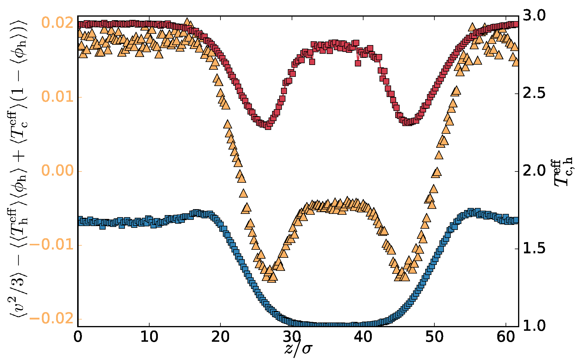
computed in each slab and averaged over the different system steady state configuration, with
being the number fraction of the hot monomers. One can also compute the average profiles of the number fractions and the effective temperature and calculate the profile of the combined quantity
. Both of these quantities are plotted in
Figure 2b. Their difference (
Figure 3) captures the correlation of the number fraction of the hot monomers and the msv. These quantities are positively correlated in the hot phase, mostly uncorrelated in the transition region, and negatively in the cold phase. This is expected since increasing the effective temperature of the hot subset should favour further segregation, increasing the hot number fraction. The correlation profile follows the effective temperature of the hot subset of the particles. Interestingly hot particles are hotter deep inside the cold phase than in the adjacent transition region and, similarly, cold chains are slightly colder in the hot phase than in the transition region (
Figure 3). To avoid excessive heat transfer, the conformation of the hot chain in the cold phase is more compact, increasing self-contacts. We confirm this by calculating the mean square gyration radius of the chains in the different regions (
Table 1). Analogous effect is observed also in equilibrium phase-separated blends, where the chains of the minority phase are more compact to decrease the unfavourable contacts with the chains of the majority phase.
In fact, deep in the bulk phase, the number fraction of hot monomers
and the msv are related by
(see
Figure 2). This is a consequence of a local flux conservation because there is no heat transport out of the region deep in the bulk phase. In the interfacial region, this relation is slightly violated, as there is a net heat transport to the surrounding areas.
To understand the directional and ensemble properties of the profiles deeper, we investigate the pressure tensor
This is derived from mechanics considerations only [
9,
17] and in the non-equilibrium case should be interpreted in the mechanical sense. For example, the trace of the tensor represents the mechanical force per unit area that the box experiences by the presence of the polymer mixture. Our particles do not have any directionality and therefore we do not need to consider any additional “active” terms that appear for vectorial activity class models [
14,
18]. The averaging in Equation (
3), as before, represents an average over the configurations characterizing the steady state.
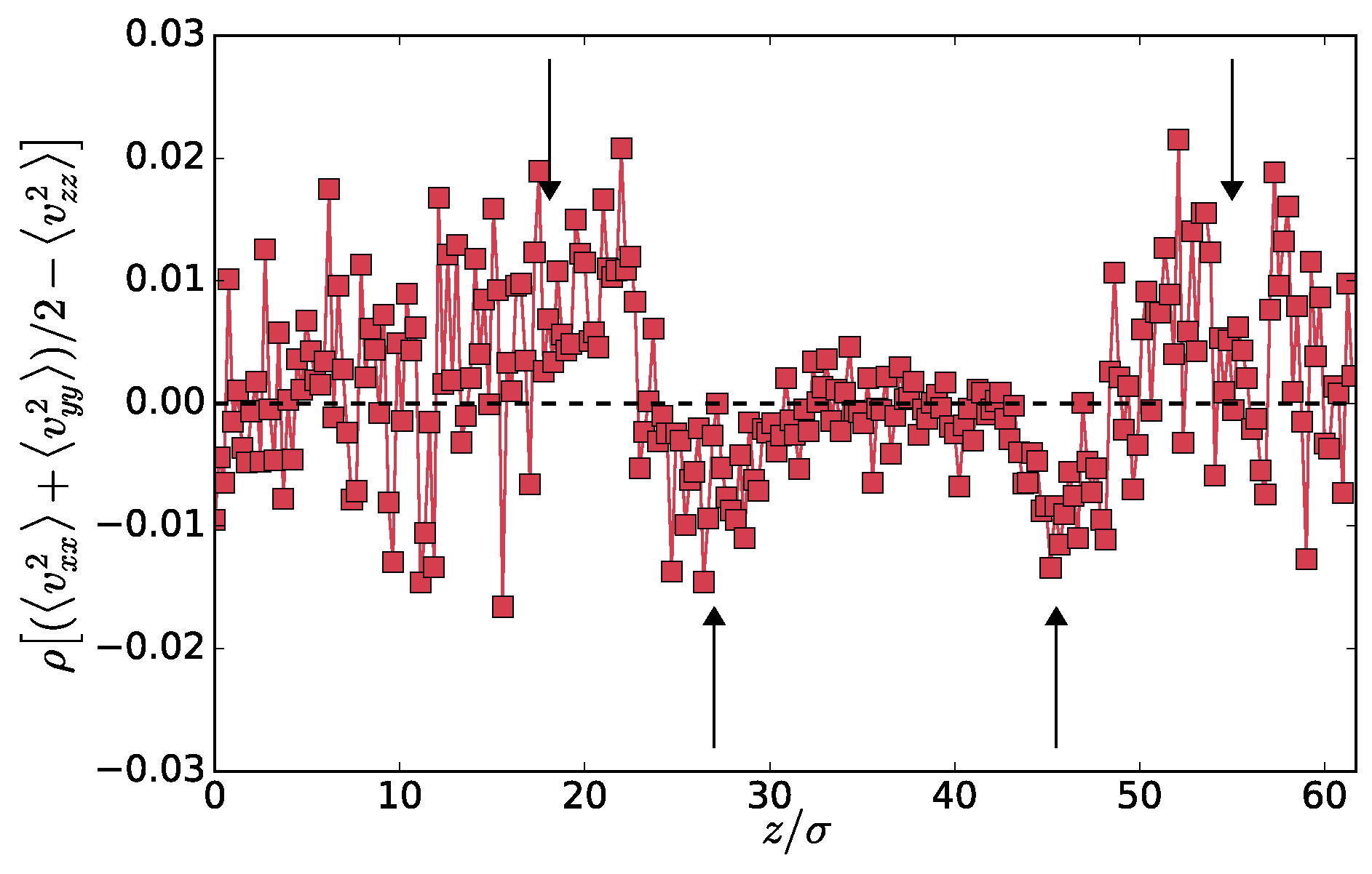
First, in
Figure 4, we plot the profile of the difference between mean tangential and normal components of the kinetic part of the pressure tensor:
. Although the data is a bit noisy, as we are now using both particles types, we can still observe a non-monotonous profile similar to the one shown in
Figure 3. This is particularly interesting in the context of the interfacial tension. In equilibrium phase separation, the interfacial tension
can be computed as
where the
and
are the normal and tangential components of the pressure tensor. The kinetic part of the pressure tensor does not contribute to
because it is constant and cancels out from the two components. Interestingly, if an analogous definition of
applies to the present non-equilibrium system, the non-monotonous profile in
Figure 4 shows that the kinetic part of the pressure tensor might contribute to
. An analogous definition of the surface tension seems to be applicable in the vectorial activity phase separation [
14,
15].
Figure 4 also shows that, very close to the interface, the distribution of the velocities is not isotropic. This also means that the velocity distributions of the hot or cold particles separately can not be Maxwellian at the interface because the
z-component has different mean squares than the other two. In the mixed phase, it was found [
10] that the two particle types preserve Maxwellian distributions. It is therefore the interface that breaks the rotational symmetry even in the momentum space, which is a pure non-equilibrium effect. The off-diagonal components of the kinetic part of the tensor are within our accuracy zero on average.
We computed the second (virial) part of the pressure tensor (
3) as detailed in [
19]. That is, the summation goes over particle pairs
n and
m connected by vector
, which intersects a mid-plane of a slab at given
z. The full pressure tensor exhibits a flat profile but unfortunately is too noisy (see
Figure A3a,b). Therefore, we can not confirm numerically that the asymmetry shown in
Figure 4 is present for the whole tensor, nor can we compute reliably the surface tension as the integral of the difference of its tangential and normal components. However, we observe that the system in the steady state is in mechanical equilibrium.
We use the plateau values of temperature, density and number fraction, in the average profiles of these quantities, to construct a phase diagram as a function of the
. In
Figure 5, we show the phase diagram for the overall density of the two phases and
Figure A4a,b shows the number fraction of the hot particles and the msv, respectively.
Based on the phase diagrams, one can try to measure an analogue of the equilibrium critical exponent,
, governing the composition difference as a function of
. From the density phase diagram (
Figure 5), we extract the difference in the phase densities
and examine it as a function of the asymmetry parameter
. We plot it in
Figure 6 in double log scale and fit the data to
, to compare it to the behavior of equilibrium phase separation. There, the order parameter (e.g., the density difference) scales with interaction strength with the exponent
from the Ising universality class, and
is found for a system in the mean-field approximation. The best fit of our data gives
,
and
. Within our precision, we could not get too close to the critical point and therefore our exponent
shows the mean-field behavior. This is typical for polymeric blends due to the extensive number of contacts for each chain (proportional to
), which effectively extend the interaction range, and the Ising behavior is observed only when the correlation length becomes much larger than the polymer gyration radius [
20]. The critical activity ratio
is a bit lower than the one found by entropy production
; however, comparably good fits can be achieved when only parameters
A and
are fitted with
set to
or when
is set to
and
A and
are fitted (see
Figure 6 for details). However, these estimates of the critical exponent and
should be taken with a grain of salt. Firstly, the density difference fluctuations are of the order of
, which is relatively high. Secondly, the choice of the order parameter should have no effect, apart from a different numerical sensitivity on the value of the exponent
. However, for example, when we take the difference of the volume fraction of the hot particles as the order parameter, we could not extract any definite range of the exponent (Inset of
Figure 6). On the other hand, our finite-size scaling analysis gives some additional support that we see
close to the mean-field exponent
. Certainly, a more detailed work is necessary to determine these and other exponents more precisely. This, however, is quite complicated in the present case as the effective interactions are asymmetric i.e., hot–hot pairs behave differently than cold-cold ones. In equilibrium phase separation, such cases are treated by the “field mixing” [
21], which relies on the equilibrium statistical mechanics inapplicable to the present case.
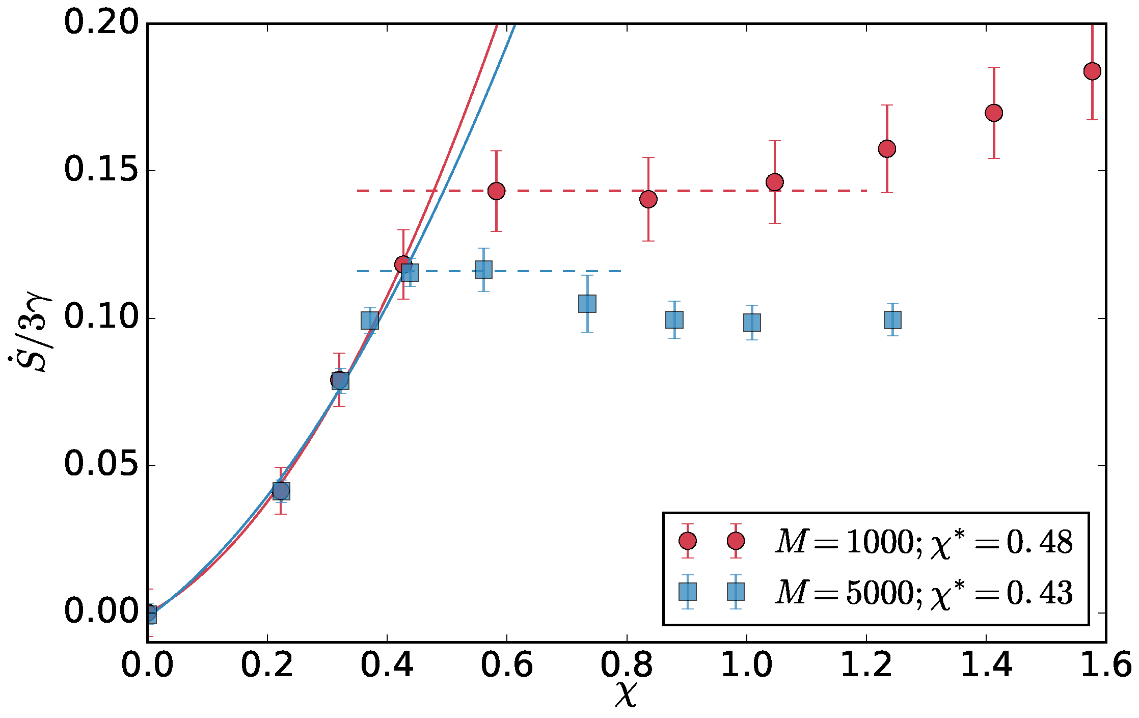
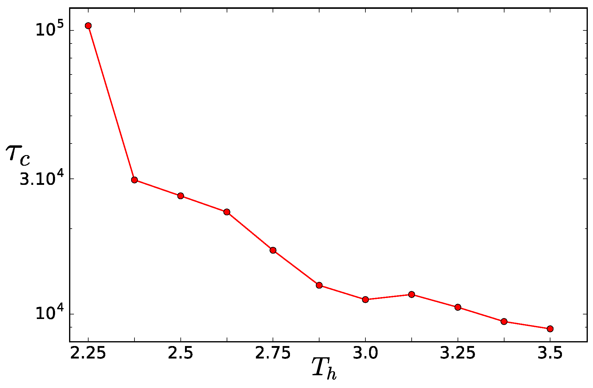
Finite Size Effects
As a first step, we want to validate the method to determine the critical temperature asymmetry using the crossover of the entropy production detailed in [
10]. There, only the entropy production of systems of
and
chains was compared to get the extent of the finite size effects. The entropy production (per hot particle)
in steady state is a sum of the contribution for each reservoir. For reservoir
i, it is the net heat flux to the reservoir per hot particle
divided by the temperature of the reservoir
per unit time. The total entropy production of the system per hot particle then reads
We measure the effective temperatures in the simulations and calculate the
as above. The entropy production per particle grows with
, until the two-dimensional interface develops in the system and then it plateaus (drops in the infinite system size limit). The
is obtained as the crossover point between these two regimes. Here, in
Figure 7, we compare two system sizes
and
.
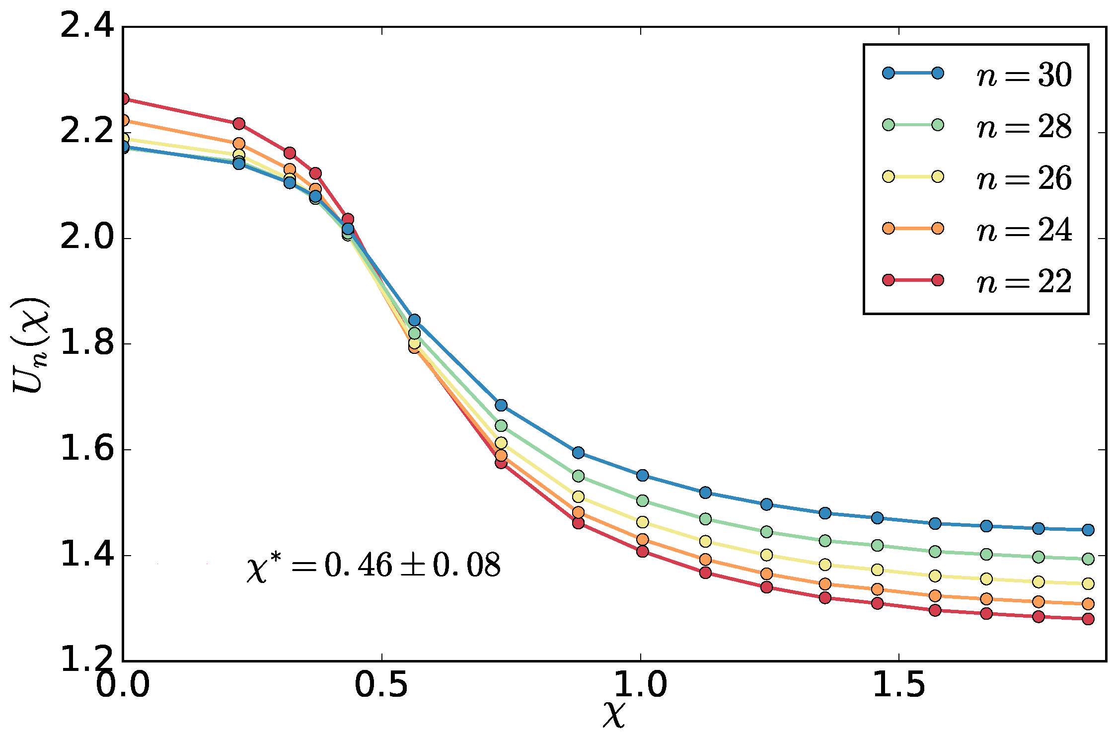
To validate the method, we extract the
using also the standard technique of the fourth order cumulant
of the density distribution in sub-boxes and compare the results of the two system sizes. The cumulant
where
is the density of the hot particles in
i-th sub-box out of total
equal sub-boxes covering the system,
is the average density of the hot particles (in our case
) and the brackets
denote average over the different conformations of the system in the steady state. We used also the density of the cold particles with the same results (not shown).
While the entropy production is affected by the choice of the fitting range above the transition point, which is affected by the finite size effects, the cumulant method relies on a proper choice of the value of
n, which determines the linear size of the sub-box
. This is to be larger than the correlation length and smaller than the overall system size, so the density fluctuations are not influenced by the fixed ratio of hot and cold particles in the system. As we don’t know these lengths a priori, we try a range of sub-box sizes for the system with
chains and look at the cumulants crossings. The average crossing point represents an estimate of the critical point and standard deviation an estimate of the error. We select a range of sub-box sizes that gives a result found from the entropy production
and use the same sub-box sizes to extract the critical point for the larger
system. The result (
Figure 8) is consistent within the error bars with the result found with the entropy production method. Relatively small sub-box sizes were used as, with our brute-force MD simulations, we could not get too close to the critical point, and, therefore, the correlation length is also limited.
The location of the crossings of the cumulants gives support to the values of the exponent
found above. It takes place around their value of about
, which is somewhat closer to the mean-field value of the equilibrium phase transition
[
22] than the value for the Ising universality class
[
23]. The exponent
is also closer to the mean-field value than the one for the Ising as discussed above. This is expected as we could not get very close to the critical point.
The different values of
for different system sizes are the consequence of the fact that
itself depends on the system size in the separated state. This is due to the fact that the interface represents a finite fraction of the finite system, the effective temperatures of the hot and cold components depend on the fraction and therefore on the system size. This is clearly visible in
Figure 9, where one also sees that, in the mixed state,
does not depend on system size.
Therefore, the cumulant technique represents only an estimate of the critical point for a given finite size system that determines the effective temperatures in the separated case. How the effective temperatures depend on system size remains an open question.
3. Capillary Waves and Interfacial Tension
In equilibrium phase separated system, one can extract the interfacial tension from the capillary wave spectrum of the interface [
24,
25,
26]. The capillary wave Hamiltonian is quadratic in the interface height gradient under the assumption of small gradients (no overhangs and bubbles). Thus, in Fourier space, it is diagonal
where
is the interfacial tension,
L is the system size and
As and
Bs are the amplitudes corresponding to the mode
. For more details, see [
25,
26] and the
Appendix A. Using the equipartition theorem, every modes carries on average energy of
and therefore the capillary wave spectrum is quadratic in inverse
q,
where we use the notation from [
25]:
and we drop the subscripts
.
In our out-of-equilibrium system, we can not write a Hamiltonian or use the equipartition theorem for capillary waves, but we can measure the spectrum of the interfacial fluctuations. The method to do so can be directly generalized for the present nonequilibrium case and is summarized in the
Appendix A. As detailed there, for analysis purposes, we examine the interface subdivided into
equal sized (
) blocks in
x- and
y-directions. This division into blocks filters out all wave vectors larger than
.
To obtain a correct spectrum, we have to take conformations separated by a time span larger than the correlation time of the slowest capillary mode (
and
, corresponding to
). We analyzed the interface position for the mode by computing its autocorrelation function
and fitting it with the exponential
. The correlation time
as a function of the thermostat temperature is plotted in
Figure 10. To get the spectrum, we only used a subset of all the configurations, i.e., configurations separated by
, which is larger than all
except for
. Contrary to [
25], the correlation time decreases with the increasing asymmetry characterized by
.
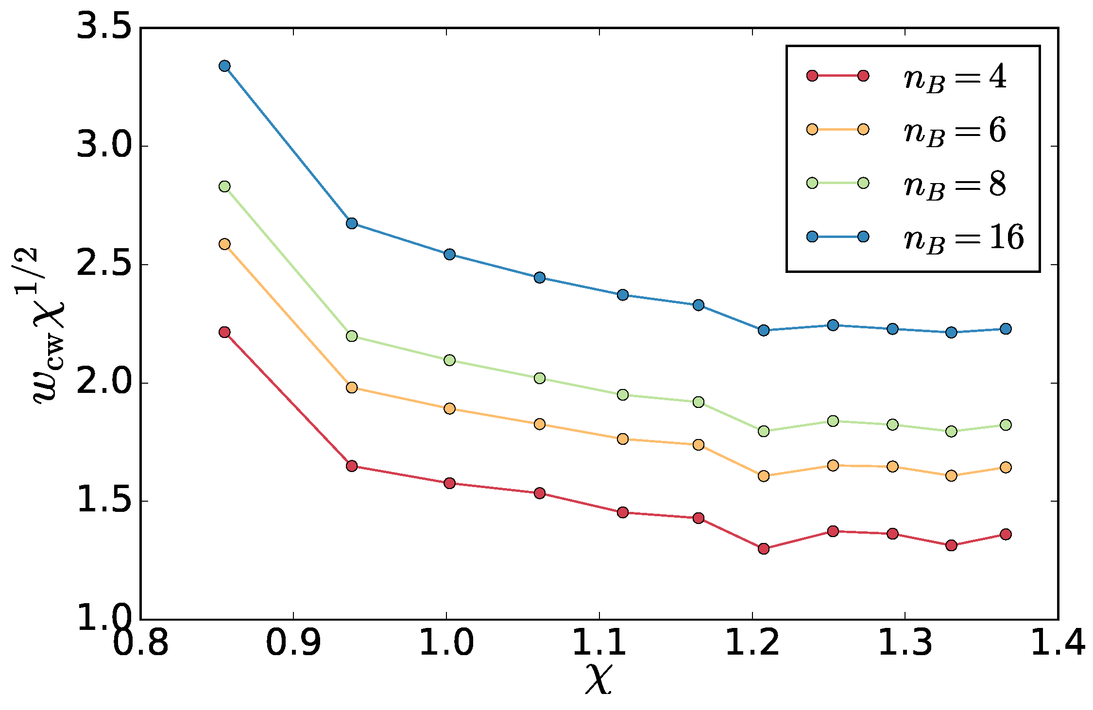
Surprisingly, we find that the amplitude is, as in equilibrium, proportional to
and independent from the block number
(
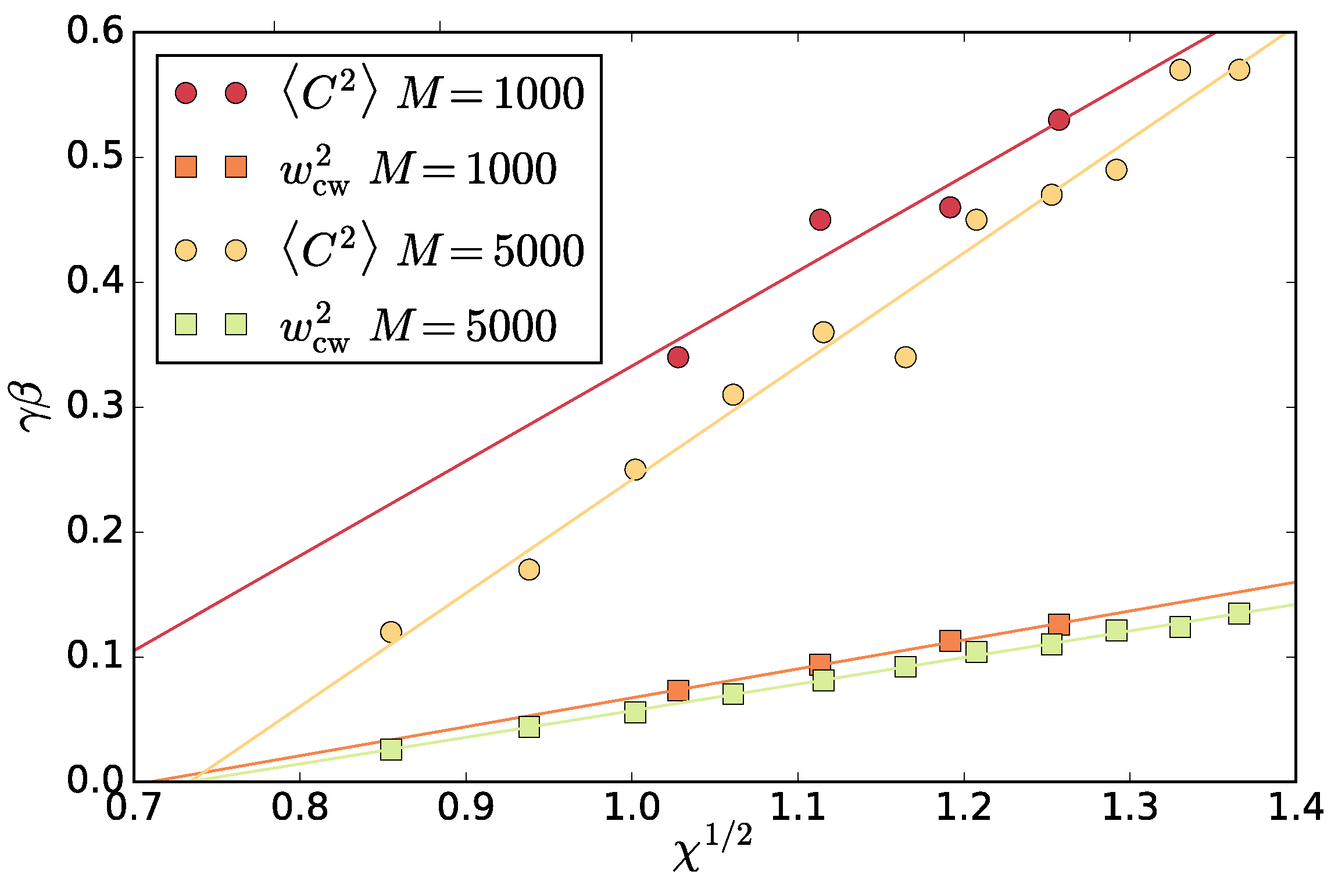
Figure 11). This allows us to use the interfacial fluctuations as a mechanistic definition of the interfacial stiffness
. One way to do this is extracting the
from a fit of (
8) to the spectrum. To ensure we are not affected by the correlations in the slowest mode, we additionally left out the slowest mode from the fit. In fact, this does not change the resulting values except for the correlated case of
. In
Figure 12, the resulting
as a function of
and
are shown.
We stress that, in equilibrium, the two symbols of interfacial stiffness
represent the product of the interfacial tension and the inverse temperature. The main result of [
14,
15] is that, for the vectorial activity separation,
is the surface tension consistent with the definition (
4), which is negative, and
corresponds to the active work dissipated to the environment, which is also negative. While the negative surface tension amplifies fluctuations, eventually leading to a surface rupture, the actively swimming particles oriented towards the surface push towards the dense phase and reform the surface again on the expense of their active work. This gives rise to the positive stiffness that governs the surface fluctuations. In the present scalar case, we cannot conclude the signs of
and
separately, but we do observe a positive interfacial stiffness and also an equilibrium-like spectrum. Although
can be related to the excess energy present in the system due to activity, there is no orientational order at the interface in the scalar case. We hypothesize that the velocity anisotropy in
Figure 4 could play a role.
An alternative way to obtain the interfacial stiffness is from the mean squared interfacial width. Because of the
dependence, the present non-equilibrium interface suffers from broadening similar to its equilibrium counterpart: The mean square width of the interface position due to capillary waves is given by
Using (
8), this can be written as an integral over wave vectors in polar coordinates
where the cutoff
is set by the smallest possible wave vector in a finite system of size
L. The cutoff
defines a length
a below which the approximation of smooth interface with small gradients is invalid. This length scale is unknown, but one can investigate the width at different resolutions by setting
. This gives
where
c is a constant.
Similarly to [
25], one could extract the interfacial stiffness also from the scaling of
with the system size. We do not use this method here because the
depends on the system size (shown in
Figure 9) and one would need to include this yet unknown dependency. For completeness, we provide in the
Appendix A an adaptation of the method for the present case of asymmetric phases and discuss where the
dependence comes into play.
In practice, using (
12), we measure the interface width as a function of the
and extract the slope in the log-linear regime (
Figure 13).
We do this for each temperature asymmetry and extract the dependence of the stiffness
on
(
Figure 12).
The different methods yield different values of interfacial stiffness. This is also observed in equilibrium systems, where the source of this discrepancy is not completely clear. It is attributed to correlation effects between subsequent interface snapshots, or the different methods inherently producing different results [
25]. The former reason seems unlikely for our case, as in our system the correlation time decreases with
(
Figure 10). The latter case is more likely. The phases in our system exhibit different densities at different
, which is an additional complication avoided in the standard work [
25]. Although we are not aware of how this difference should be incorporated at the level of
, it can not be denied that it has an effect on the resulting value of
, which would agree with the fact that the discrepancy is growing with
. Nevertheless, the trends for both methods are the same: the interfacial stiffness scales linearly with
, which is again reminiscent of the equilibrium case. This is more visible for the
method, which is less noisy as the values are obtained from a two parameter fit (
c and
) instead of one in the amplitude case.
From the linear fit of
versus
, we can extract another estimate of the critical asymmetry as
. Both methods give the same value
, which gives credence to our analysis. This value of
, agrees, within errorbars, with the one obtained from the cumulant method above (
). Additionally, in
Figure A6, we compare the present interfacial stiffness dependence with one obtained for a smaller system with
. The values and the location of
obtained from the width analysis agree very well with the ones found for the larger system.
From the analysis above and
Figure 13, we also obtained the width of the interface as a function of the temperature asymmetry
. This is plotted in
Figure 14 for various block numbers
from the linear regime of
Figure 13 (see also
Figure A5 in the
Appendix B for plot with respect to
). The width values depend on
, but the profile is universal, and, for large
, it approaches
dependence. This is the same as the dependence found for equilibrium phase separation with two polymer species characterized by Flory parameter
. The latter can be understood by a simple scaling argument: the energy of a loop of polymer A in the B phase gets an energy penalty of
. In equilibrium, this must be of the order of
and therefore we have
. As the width of the interface is proportional to the size of this loop
, we get the result above [
27]. In the non-equilibrium case, we hypothesize that a typical magnitude of the fluctuations of the entropy production gives rise to a loop size as
, which gives the same behavior of the interface width as in equilibrium.
4. Discussion
In this work, we examine a scalar active-passive (two-temperature) polymer mixture that for high-enough temperature asymmetry exhibits non-equilibrium phase separation. At first, we show that the system has low sensitivity to the chosen friction when studied using the effective temperatures in form of the asymmetry parameter of the two components. Still, a small variation of the order parameter with remains, which poses a question of the existence of a truly unifying description of systems with different frictions.
Using aligned, well-separated systems, we extract the spatial profiles of kinetic and static properties such as mean square velocities and densities. In contrast to the equilibrium behavior, analysis of the pressure tensor profile reveals that its kinetic part can contribute to the interfacial tension. Based on the profiles, we construct phase diagrams that can further be used to extract the critical exponents governing the transition. While our preliminary study suggests the related critical exponent to be between the equilibrium mean-field value and the Ising universality class , its exact value and the value of other critical exponents require a more detailed study. However, the complication lies in the asymmetry of the effective interactions. The equilibrium approach is to study the transition in a grand-canonical ensemble along with the use of histogram re-weighting and field mixing methods. Here, equilibrium statistics is violated, and new analogous methods would first have to be developed to allow for an accurate universality classification of the transition.
We determine the critical asymmetry
in our system using various methods: (i) density based fourth order cumulant; (ii) extrapolation of critical density difference; (iii) analysis of capillary waves amplitudes and (iv) interfacial width. We find consistent results with the entropy production crossover method introduced in [
10].
We perform the analysis of the interfacial fluctuations and find again scaling of the interfacial stiffness and interfacial width
similar to equilibrium mixtures with lower critical solution temperature. The works [
14,
16] with vectorial activity assumed the equipartition theorem and therefore also the equilibrium-like capillary waves spectrum. Here, we explicitly construct the spectrum for scalar activity and find its equilibrium like nature. The very fact that we obtain equilibrium-like spectrum suggests an existence of some sort of equipartition theorem source, which remains unknown. It is interesting that both the vectorial and scalar activity models exhibit similar properties of the interfacial fluctuations. This suggests that a unifying description of these fundamentally different out-of-equilibrium systems might be possible. Therefore , determining the origin of the equilibrium-like fluctuations certainly deserves attention in future. A step in this direction could be to find out whether the interfacial stiffness derived from the capillary waves and related interfacial tension are relevant in the nucleation kinetics.


