Non-Gaussian Systems Control Performance Assessment Based on Rational Entropy


Abstract
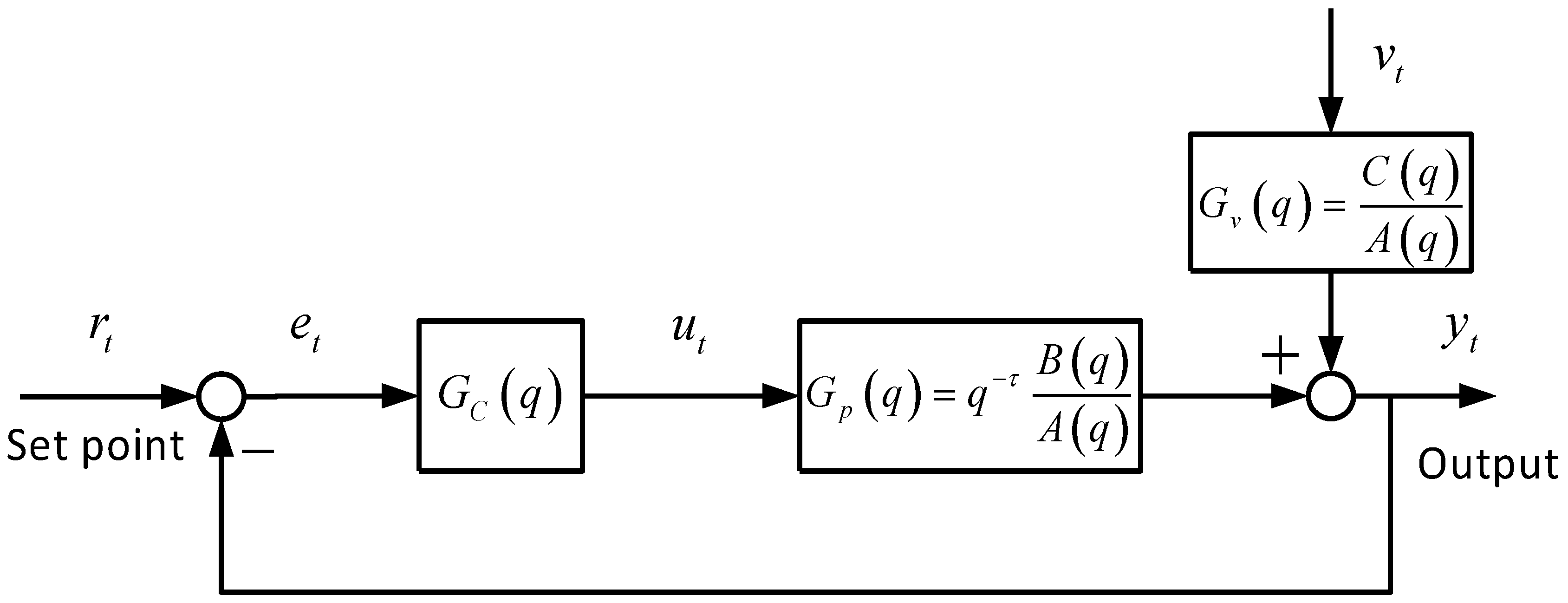
:1. Introduction
2. Minimum Entropy Control
2.1. MEC Index
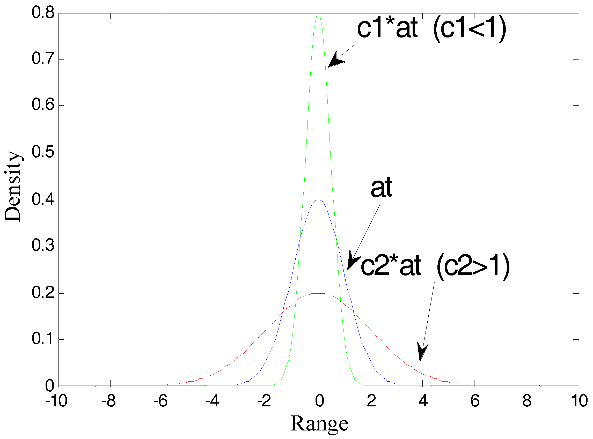
2.2. Rational Entropy
- (1)
- Select the time-series-model type. Determine/estimate the system time delay τ and system order.
- (2)
- Identify the closed-loop model from collected output samples.
- (3)
- Estimate the benchmark entropy of process data.
- (4)
- Compute the performance index.
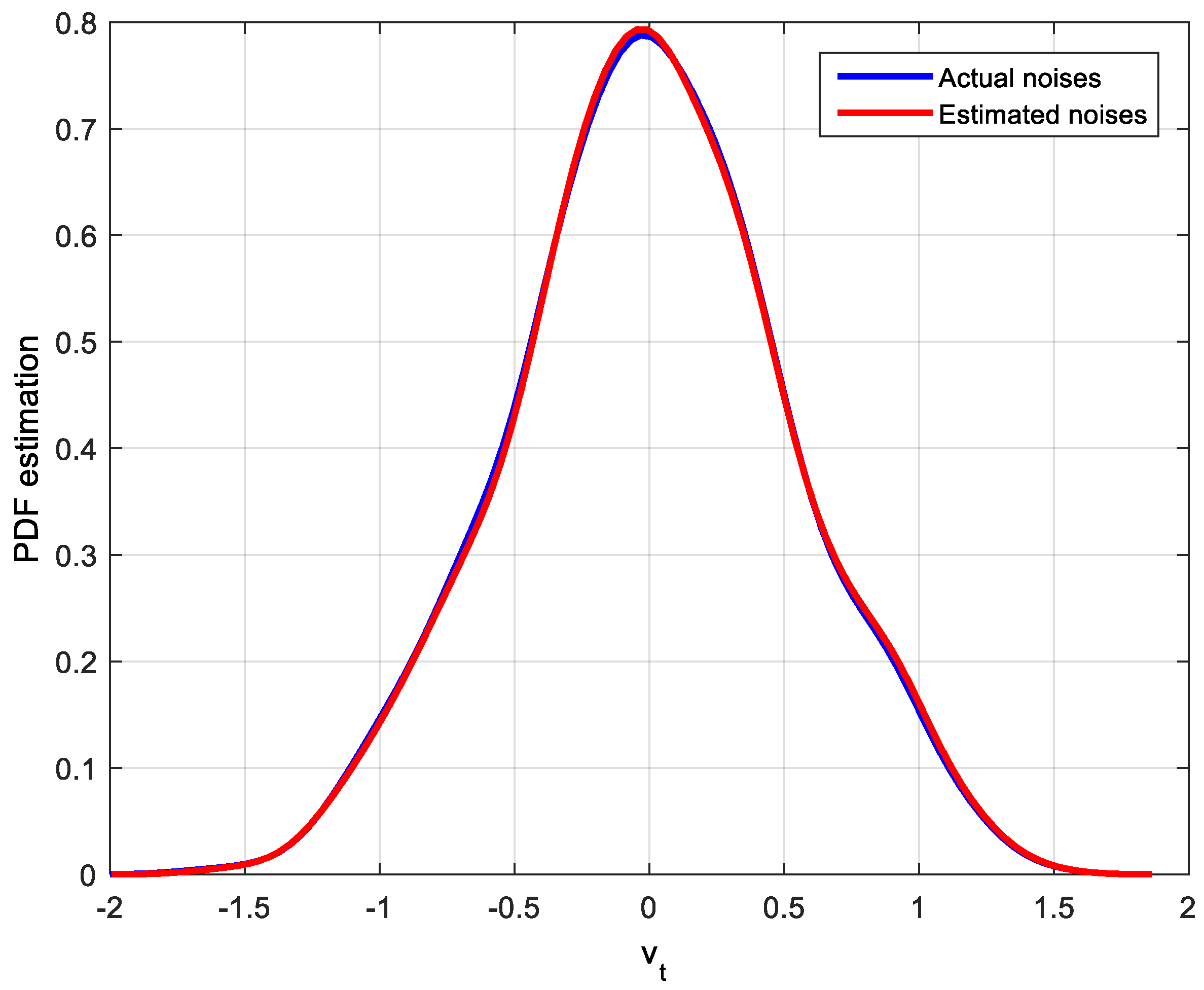
3. System Identification and Noise PDF Estimation
- (1)
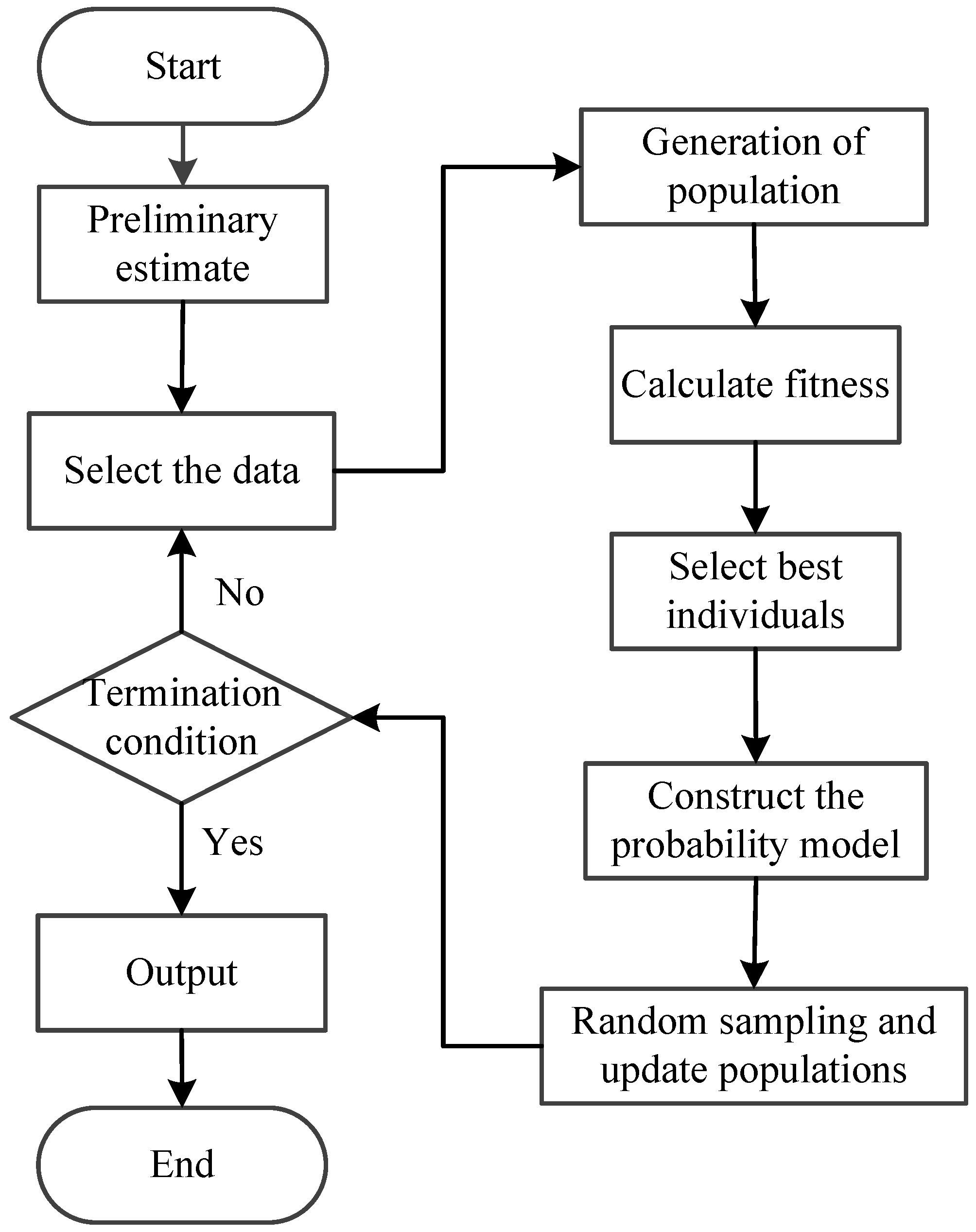
- Preliminary estimation. Rough estimation parameters are obtained by recursive maximum likelihood method. Then the task of initializing the parameters space can be accomplished with a uniform distribution using the initial value of parameter as the value range.
- (2)
- Screen seeds. From the first generation randomly select group seed from the parameter space and calculate the mean value of the residuals. Remove the seeds whose mean value is more than and keep the seeds whose mean value is less than . If the number of reserved seeds is less than , re-sampling is performed until the number of seeds retained is not less than and then the seeds reserved are collected in new parameter spaces .
- (2)
- Calculate fitness. Randomly create individuals from the parameter space . The error entropy of the parameter vector in is estimated based on the selected training data set .
- (4)
- Select superior individuals based on the cost function and estimate PDF based on the error entropy extracted from the selected individuals.
- (5)
- Calculate the estimated average value of the selected parameters and establish the probability models.
- (6)
- Set and resample individuals from the updated PDF.
- (7)
- Go to step 2 until the stopping criterion is met. This process can be represented by Figure 3.
4. Simulation
4.1. Parameters and CPA Index Estimation with Fixed Controller and Unimodal Distribution Noises
- (1)
- Normal distribution
- (2)
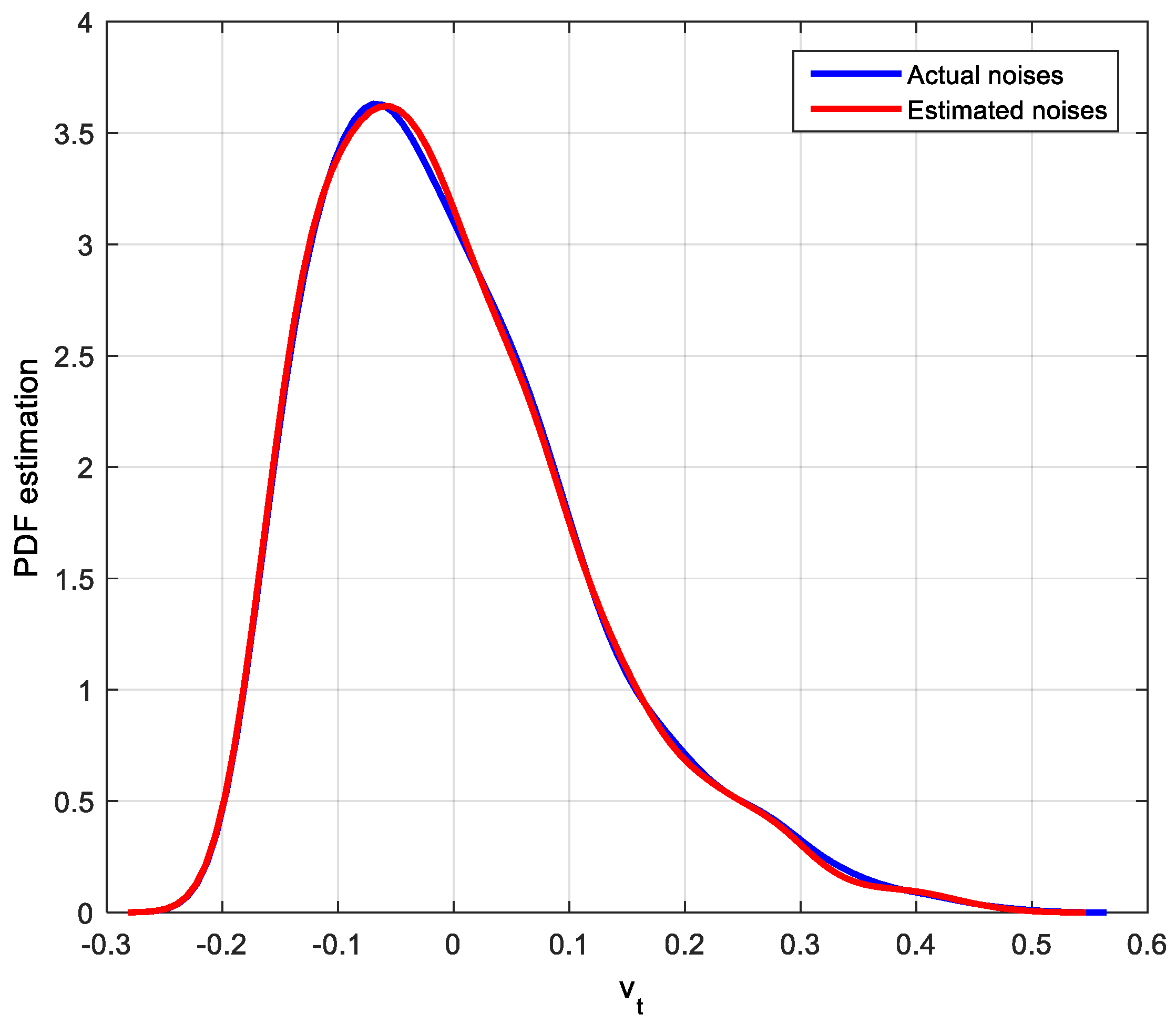
- Beta distribution
- (3)
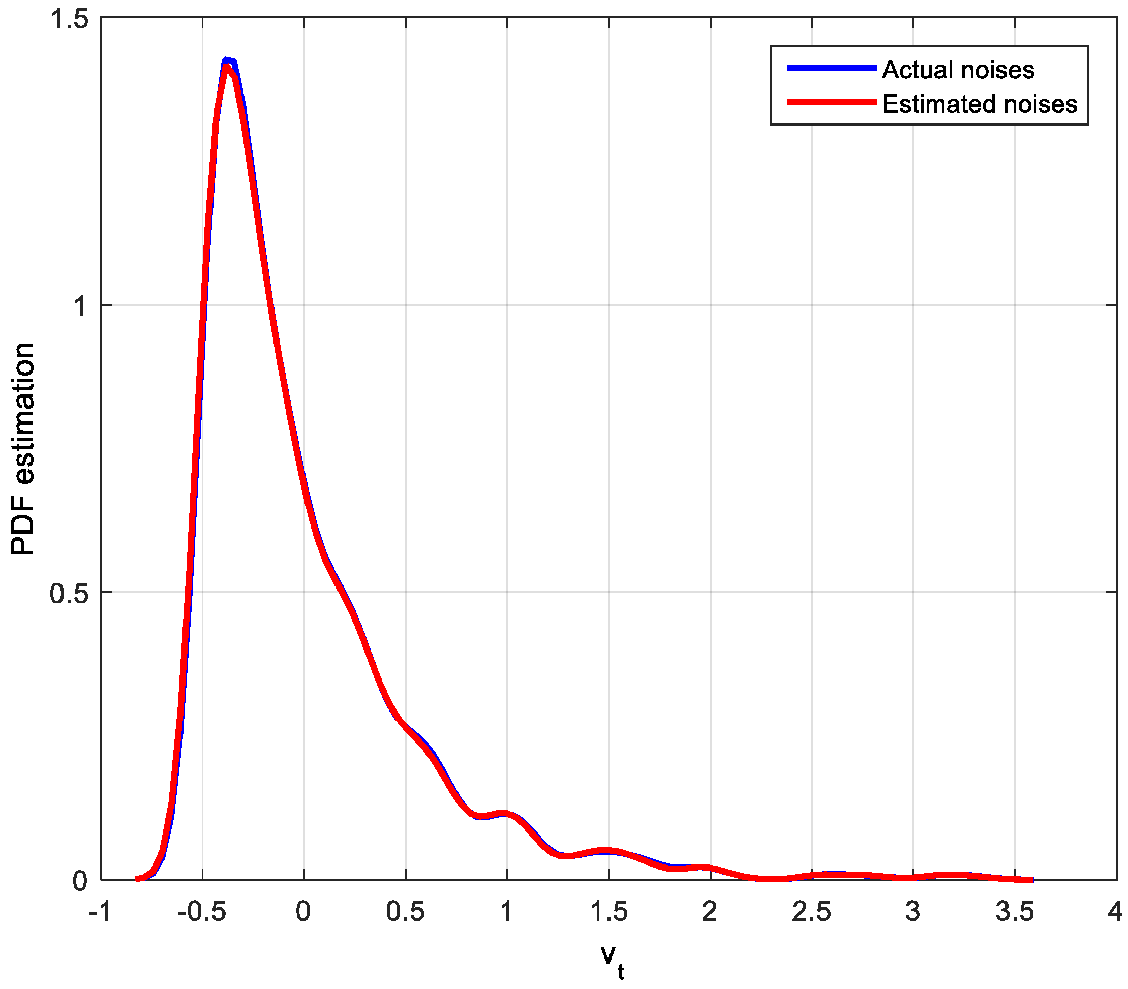
- Exponential distribution
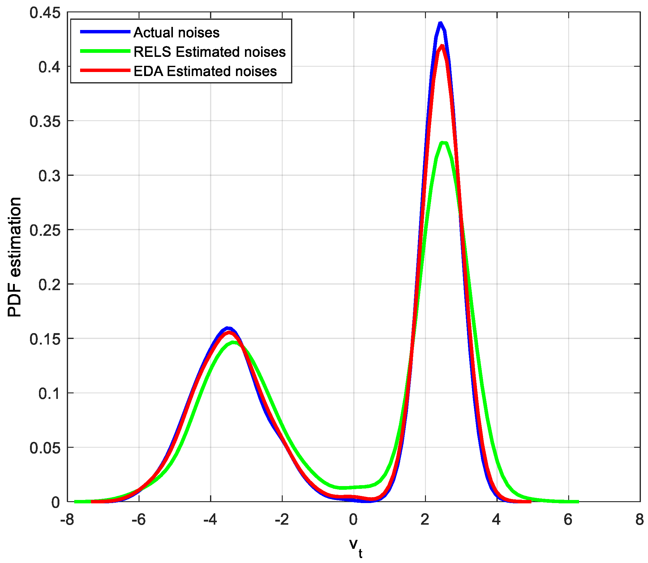
4.2. Parameters and CPA Index Estimation with Fixed Controller and Bimodal Distribution Noises
- (1)
- (2)
- (3)
4.3. CPA Index with Different Gain Controllers
5. Conclusions
Author Contributions
Funding
Conflicts of Interest
References
- Khamseh, S.A.; Sedigh, A.K.; Moshiri, B.; Fatehi, A. Control performance assessment based on sensor fusion techniques. Control Eng. Pract. 2016, 49, 14–28. [Google Scholar] [CrossRef]
- Jelali, M. Control Performance Management in Chemical Automation; Springer: London, UK, 2013. [Google Scholar]
- Astrom, K.J. Introduction to Stochastic Control Theory; Academic Press: New York, NY, USA, 1970. [Google Scholar]
- Harris, T.J. Assessment of control loop performance. Can. J. Chem. Eng. 1989, 67, 856–861. [Google Scholar] [CrossRef]
- Huang, B.; Shah, S.L. Performance Assessment of Nonminimum Phase Systems. Performance Assessment of Control Loops; Springer: London, UK, 1999. [Google Scholar]
- Huang, B. Minimum variance control and performance assessment of time-variant processes. J. Process Control 2002, 12, 707–719. [Google Scholar] [CrossRef]
- Chen, J.; Wang, W.Y. Performance assessment of multivariable control systems using PCA control charts. In Proceedings of the IEEE Conference on Industrial Electronics and Applications (ICIEA 2009), Xi’an, China, 25–27 May 2009. [Google Scholar]
- Grimble, M.J. Controller performance benchmarking and tuning using generalised minimum variance control. Automatica 2002, 38, 111–119. [Google Scholar] [CrossRef]
- Saha, P. Performance Assessment of Control Loops: Theory and Applications; Springer: Berlin/Heidelberg, Germany, 1999. [Google Scholar]
- Pour, N.D.; Huang, B.; Shah, S.L. Performance assessment of advanced supervisory–regulatory control systems with subspace LQG benchmark. Automatica 2010, 46, 1363–1368. [Google Scholar] [CrossRef]
- Kadali, R.; Huang, B. Controller performance analysis with LQG benchmark obtained under closed loop conditions. ISA Trans. 2002, 41, 521. [Google Scholar] [CrossRef]
- Julien, R.H.; Foley, M.W.; Cluett, W.R. Performance assessment using a model predictive control benchmark. J. Process Control 2004, 14, 441–456. [Google Scholar] [CrossRef]
- Sotomayor, O.A.; Odloak, D. Performance assessment of model predictive control systems. IFAC Proc. Vol. 2006, 39, 875–880. [Google Scholar] [CrossRef]
- Schäfer, J.; Cinar, A. Multivariable MPC system performance assessment, monitoring, and diagnosis. J. Process Control 2004, 14, 113–129. [Google Scholar] [CrossRef]
- Domański, P.D.; Ławryńczuk, M. Assessment of the GPC Control Quality Using Non–Gaussian Statistical Measures. Int. J. Appl. Math. Comput. Sci. 2017, 27, 291–307. [Google Scholar] [CrossRef]
- Srinivasan, B.; Spinner, T.; Rengaswamy, R. Control loop performance assessment using detrended fluctuation analysis (DFA). Automatica 2012, 48, 1359–1363. [Google Scholar] [CrossRef]
- Pillay, N.; Govender, P. A Data Driven Approach to Performance Assessment of PID Controllers for Setpoint Tracking. DAAAM Int. Symp. Intell. Manuf. Autom. 2013, 69, 1130–1137. [Google Scholar] [CrossRef]
- Qin, S.J. Control performance monitoring—A review and assessment. Comput. Chem. Eng. 1998, 23, 173–186. [Google Scholar] [CrossRef]
- Harris, T.J.; Seppala, C.T.; Desborough, L.D. A review of performance monitoring and assessment techniques for univariate and multivariate control systems. J. Process Control 1999, 9, 1–17. [Google Scholar] [CrossRef]
- Jelali, M. An overview of control performance assessment technology andchemical applications. Control Eng. Pract. 2006, 14, 441–466. [Google Scholar] [CrossRef]
- Yue, H.; Zhou, J.; Wang, H. Minimum entropy control of B-spline PDF systems with mean constraint. Automatica 2006, 42, 989–994. [Google Scholar] [CrossRef]
- Wang, H. Minimum entropy control of non-Gaussian dynamic stochastic systems. IEEE Trans. Autom. Control 2002, 47, 398–403. [Google Scholar] [CrossRef]
- Wang, H. Bounded Dynamic Stochastic Systems: Modelling and Control; Springer: London, UK, 2000. [Google Scholar]
- Zhou, J.L.; Wang, X.; Zhang, J.F.; Wang, H.; Yang, G.H. A New Measure of Uncertainty and the Control Loop Performance Assessment for Output Stochastic Distribution Systems. IEEE Trans. Autom. Control 2015, 60, 2524–2529. [Google Scholar] [CrossRef]
- Zhang, J.; Jiang, M.; Chen, J. Minimum entropy-based performance assessment of feedback control loops subjected to non-Gaussian disturbances. J. Process Control 2014, 24, 1660–1670. [Google Scholar] [CrossRef]
- Zhang, J.; Zhang, L.; Chen, J.; Xu, J.; Li, K. Performance assessment of cascade control loops with non-Gaussian disturbances using entropy information. Chem. Eng. Res. Des. 2015, 104, 68–80. [Google Scholar] [CrossRef]
- You, H.; Zhou, J.; Zhu, H.; Li, D. Performance assessment based on minimum entropy of feedback control loops. In Proceedings of the IEEE Data Driven Control and Learning Systems Conference, Chongqing, China, 26–27 May 2017. [Google Scholar]
- Meng, Q.W.; Fang, F.; Liu, J.Z. Minimum-Information-Entropy-Based Control Performance Assessment. Entropy 2013, 15, 943–959. [Google Scholar] [CrossRef]
- Giffin, A. Maximum Entropy: The Universal Method for Inference. arXiv, 2009; arXiv:0901.2987. [Google Scholar]
- Caticha, A. Relative Entropy and Inductive Inference. Am. Inst. Phys. 2004, 707, 75–96. [Google Scholar]
- Chan, Y.T.; Wood, J. A new order determination technique for ARMA processes. IEEE Trans. Acoust. Speech Signal Process. 1984, 32, 517–521. [Google Scholar] [CrossRef]
- Svante, B.; Ljung, L. A Survey and Comparison of Time-Delay Estimation Methods in Linear Systems; Division of Automatic Control, Department of Electrical Engineering, Linkoping University: Linkoping, Sweden, 2003. [Google Scholar]


| 0.8396 | 0.8256 | 0.8282 | |
| 0.8416 | 0.8251 | 0.8282 | |
| 0.9457 | 0.9375 | 0.9400 | |
| 0.9464 | 0.9452 | 0.9417 |
| 0.9447 | 0.9201 | 0.9323 | |
| 0.9359 | 0.9176 | 0.9294 |
| 1.0000 | 0.9903 | 0.9611 | 0.9096 | 0.8186 | ||
| 1.0060 | 0.9965 | 0.9669 | 0.9151 | 0.8238 | ||
| 0.9999 | 0.9829 | 0.9369 | 0.8625 | 0.7418 | ||
| 1.0094 | 0.9932 | 0.9464 | 0.8718 | 0.7487 | ||
| bimodal | 1.0001 | 0.8971 | 0.8188 | 0.7725 | 0.7615 | |
| 1.0540 | 0.9336 | 0.8539 | 0.8033 | 0.8044 | ||
| bimodal | 0.9992 | 0.9142 | 0.8616 | 0.8479 | 1.0216 | |
| 1.0389 | 0.9430 | 0.8948 | 0.8853 | 1.0688 | ||
| bimodal | 0.9999 | 0.9487 | 0.9106 | 0.9161 | 1.0901 | |
| 1.0170 | 0.9674 | 0.9210 | 0.9302 | 1.1060 |
| 1.0000 | 0.9979 | 0.9924 | 0.9829 | 0.9667 | ||
| 0.9953 | 0.9933 | 0.9878 | 0.9783 | 0.9622 | ||
| 1.0000 | 0.9967 | 0.9883 | 0.9747 | 0.9353 | ||
| 0.9960 | 0.9927 | 0.9844 | 0.9708 | 0.9496 | ||
| bimodal | 1.0000 | 0.9746 | 0.9482 | 0.9271 | 0.9064 | |
| 1.0010 | 0.9761 | 0.9509 | 0.9302 | 0.9098 | ||
| bimodal | 1.0000 | 0.9776 | 0.9592 | 0.9457 | 0.9309 | |
| 1.0009 | 0.9800 | 0.9611 | 0.9475 | 0.9330 | ||
| bimodal | 1.0000 | 0.9855 | 0.9712 | 0.9606 | 0.9481 | |
| 0.9998 | 0.9854 | 0.9713 | 0.9612 | 0.9488 |
| 0.9999 | 0.9607 | 0.9477 | 0.8286 | 0.7169 | ||
| 0.9981 | 0.9429 | 0.9421 | 0.8178 | 0.7124 | ||
| 0.9919 | 0.9512 | 0.9310 | 0.8242 | 0.7102 | ||
| 0.9871 | 0.9405 | 0.9212 | 0.8095 | 0.7260 | ||
| bimodal | 0.9944 | 0.9833 | 0.9350 | 0.8821 | 0.7210 | |
| 0.9925 | 0.9741 | 0.9350 | 0.8767 | 0.7158 | ||
| bimodal | 0.9978 | 0.9618 | 0.9209 | 0.8626 | 0.7481 | |
| 0.9982 | 0.9589 | 0.9194 | 0.8644 | 0.7495 | ||
| bimodal | 0.9989 | 0.9819 | 0.9207 | 0.8996 | 0.7299 | |
| 0.9987 | 0.9798 | 0.9212 | 0.8994 | 0.7289 |
| 0.9389 | 0.9394 | 0.9281 | 0.9000 | ||
| 0.9477 | 0.9208 | 0.9169 | 0.9186 | ||
| 0.9428 | 0.9391 | 0.9026 | 0.8055 | ||
| 0.9357 | 0.9250 | 0.8901 | 0.8021 | ||
| bimodal | 0.9816 | 0.9591 | 0.9423 | 0.9042 | |
| 0.9802 | 0.9560 | 0.9562 | 0.9117 |
© 2018 by the authors. Licensee MDPI, Basel, Switzerland. This article is an open access article distributed under the terms and conditions of the Creative Commons Attribution (CC BY) license (http://creativecommons.org/licenses/by/4.0/).
Share and Cite
Zhou, J.; Jia, Y.; Jiang, H.; Fan, S. Non-Gaussian Systems Control Performance Assessment Based on Rational Entropy. Entropy 2018, 20, 331. https://doi.org/10.3390/e20050331
Zhou J, Jia Y, Jiang H, Fan S. Non-Gaussian Systems Control Performance Assessment Based on Rational Entropy. Entropy. 2018; 20(5):331. https://doi.org/10.3390/e20050331
Chicago/Turabian StyleZhou, Jinglin, Yiqing Jia, Huixia Jiang, and Shuyi Fan. 2018. "Non-Gaussian Systems Control Performance Assessment Based on Rational Entropy" Entropy 20, no. 5: 331. https://doi.org/10.3390/e20050331
APA StyleZhou, J., Jia, Y., Jiang, H., & Fan, S. (2018). Non-Gaussian Systems Control Performance Assessment Based on Rational Entropy. Entropy, 20(5), 331. https://doi.org/10.3390/e20050331