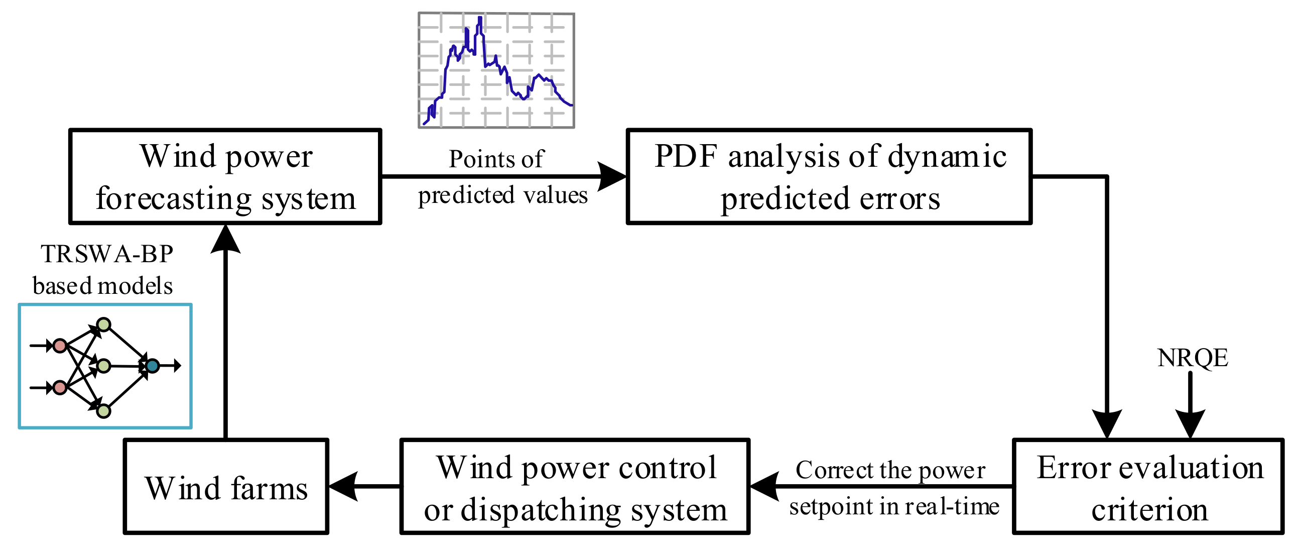
TRSWA-BP Neural Network for Dynamic Wind Power Forecasting Based on Entropy Evaluation


Abstract
1. Introduction
2. Modeling for TRSWA-BP Combined with EMD and PSR
2.1. Construction of the TRSWA-BP
2.1.1. Optimized Weight Iteration Calculation Based on the TRSWA
- Initialization is required at this stage, where the input data, including population size Dim, the maximum iteration Kmax, the temporary local network size ni, the search probability of local short-range connection Ps, the size of node neighborhood radius Rs and the maximum stored number of tabu list Ts, are defined. Furthermore, set the number of the current iterations as k = 1.
- Generate M (M > Dim) real-coded nodes by the Logistic chaotic map randomly, and calculate the fitness value of the objective function for each node. Find Dim optimal nodes among them as the initial population of node set for the TRSWA.
- Store the searched nodes in the tabu list.
- For each node of each generation in the node set of Dim population, there are ni searches of short-distance and random long-distance. Generate a random number Tm. If Tm < Ps, perform a local short-distance search, otherwise carry out a random long-distance search. Results are compared with the saved nodes in tabu list. If the results are in the list, search again. Calculate the updated objective function and find out the optimal node set.
- Generate a new node set, and calculate its objective function. The new node set is compared with the optimal one that has been generated in step (4), and then finds out the optimal set of the nodes. Record its location and the value of optimal fitness.
- Check the convergence criteria. If it is satisfied, end calculation. Otherwise, let k = k + 1 and return to step 3.
2.1.2. Modeling Process of the TRSWA-BP
- Determine the number of input and output nodes and the number of hidden layers and nodes in each hidden layer for the TRSWA-BP. Fix the set of training samples, and suppose k = 1.
- Set parameters for the BP, such as learning rate η and inertia coefficient α.
- Build an objective function through the training set, and the optimal weights of the BP are trained by the TRSWA.
- Set k = k + 1. Remove the earliest set from training samples, and add a newly acquired set into it. Repeat steps 3 and 4 until the termination condition is satisfied, and a TRSWA-BP with the best weights is established.
2.2. TRSWA-BP Combined with EMD
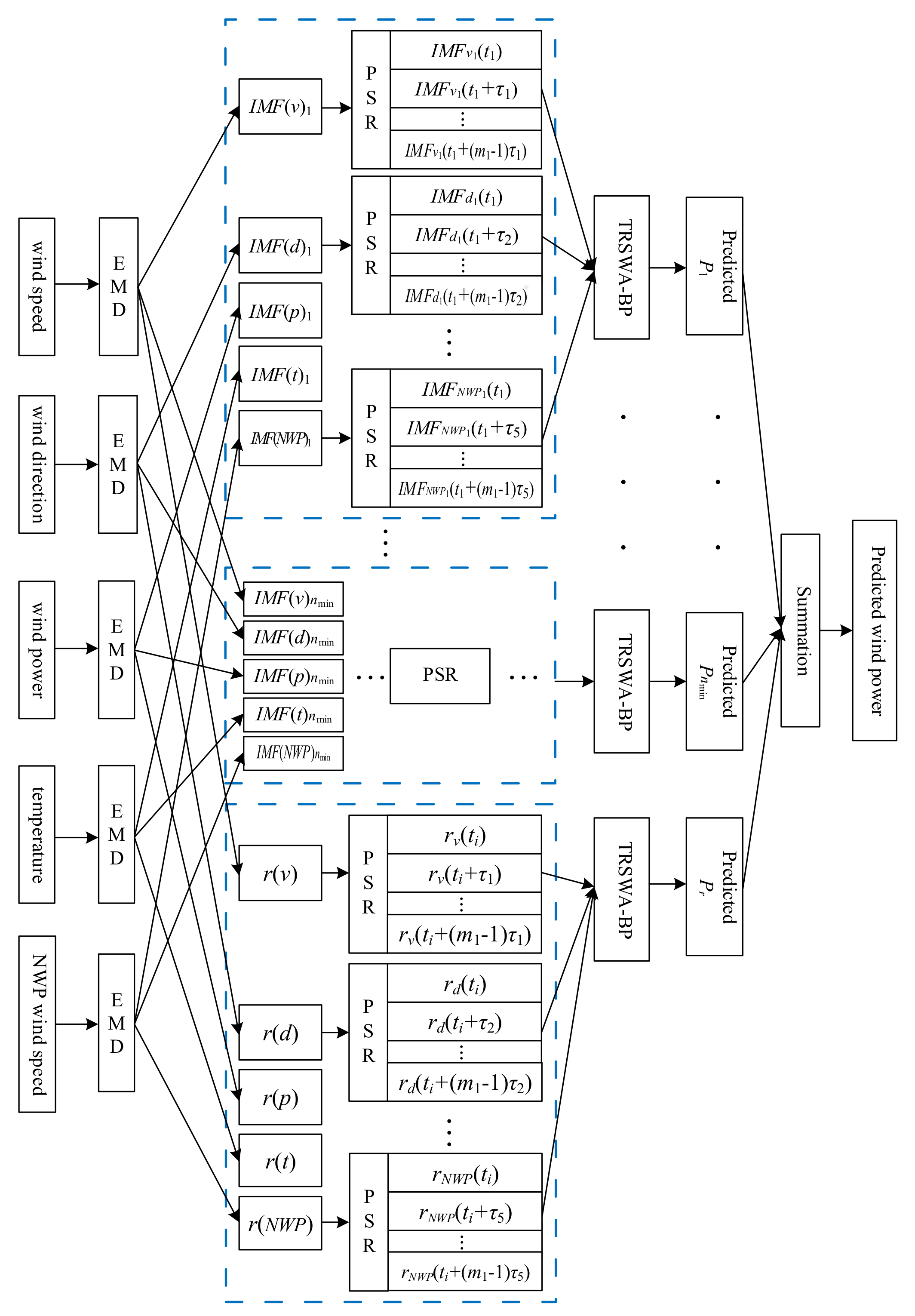
- Select data sequences, of which the length is N, including wind speed v(ti), wind direction d(ti), wind power p(ti), temperature tep(ti), and NWP wind speed denoted by vNWP(ti), i = 1, 2, …, N. Set k = 1.
- v(t), d(t), p(t), tep(t), and vNWP(t) are respectively decomposed by EMD first, whose principle is in the order of frequency from high to low. The intrinsic modal function (IMF) of nv, nd, np, nt, and nNWP layers, as well as a residual component r(·), are attained. They are denoted as IMF(v)1, …, IMF(v)nv, r(v), IMF(d)1, …, IMF(d)nd, r(d), IMF(p)1, …, IMF(p)np, r(p), IMF(t)1, …, IMF(t)nt, rt(t), and IMF(NWP)1, …, IMF(NWP)nNWP, r(NWP).
- As the number of nv, nd, np, nt, and nNWP may be unequal due to the decomposition, the minimum number nmin of them is taken as the number of the unified IMF layers of the five sequences.
- If nv > nmin in the data sequence of wind speed v(t), add all the IMF(v) behind the nminth layer together with IMF(v)nmin, to form a new IMF(v)’nmin, which means that IMF(v)’nmin = IMF(v)nmin + IMF(v)(nmin+1) + … + IMF(v)nv, (nv = 1, 2, 3, ..., nmin, …, nv). The other four sequences are treated the same way, except one (or those) when n* = nmin. Finally, the new unified sequences are obtained according to the decomposed layers. They are IMF(v)1, IMF(d)1, IMF(p)1, IMF(t)1, IMF(NWP)1; IMF(v)2, IMF(d)2, IMF(p)2, IMF(t)2, IMF(NWP)2; …, IMF(v)’nmin, IMF(d)’nmin, IMF(p)’nmin, IMF(t)’nmin, IMF(NWP)’nmin; and r(v), r(d), r(p), rt(t), r(NWP).
- Use the first N − 1 data of each layer’s new unified sequence, to train several forecasting models of TRSWA-BP, respectively. The best weights are obtained by the TRSWA (See Section 2.1.2), which are employed to predict the forecasted wind power P of each decomposed layer. They are denoted by P1, P2, P3, …, Pnmin, and Pr.
- To compose the predictions of each layer, we obtain the fitting wind power at the k moment, which is given by Pk = P1 + P2 + … + Pnmin + Pr.
- Set k = k + 1. A set of newly predicted wind power P is used as a known value to the training set, while the earliest set of data sequences is removed. Check whether it reaches the termination condition. If not, return to step (2), otherwise stop calculation.
2.3. TRSWA-BP Combined with PSR
- Select the same five sequences as step 1 in Section 2.2.
- Determine the m and τ of the above sequences through the C-C method.
- The sequences of v(ti), d(ti), p(ti), tep(ti), and vNWP(ti) are reconstructed, respectively, based on Equation (5), into the following sequences:
- 4.
- Set k = k + 1. Add the new actual value into the time series and replace the earliest one to form scrolling sequences over time. Repeat steps 2 to 5 until the termination condition is satisfied.
2.4. TRSWA-BP Combined with EMD-Based PSR
3. Entropy Evaluation for Error Sequence on Non-Gaussian Property
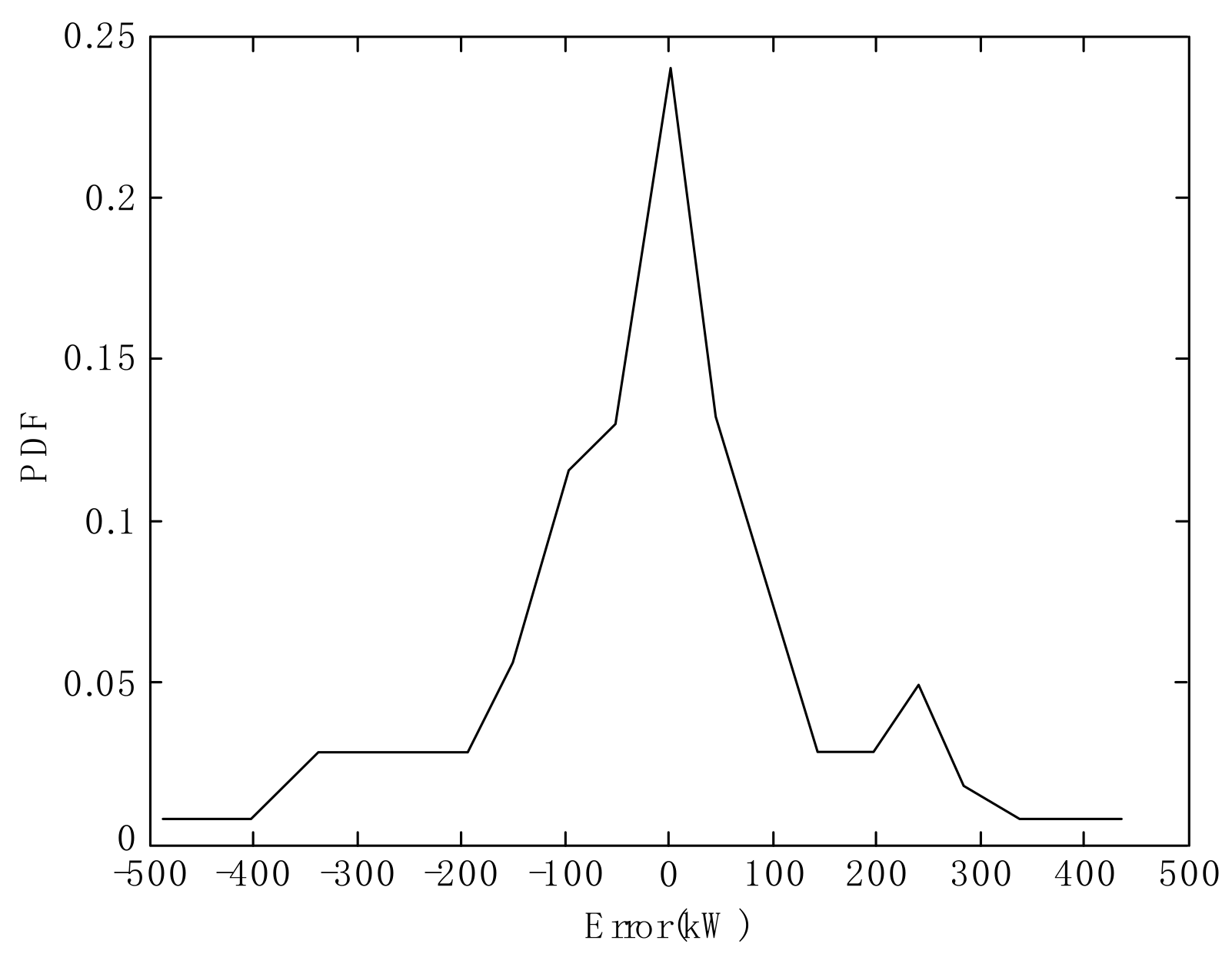
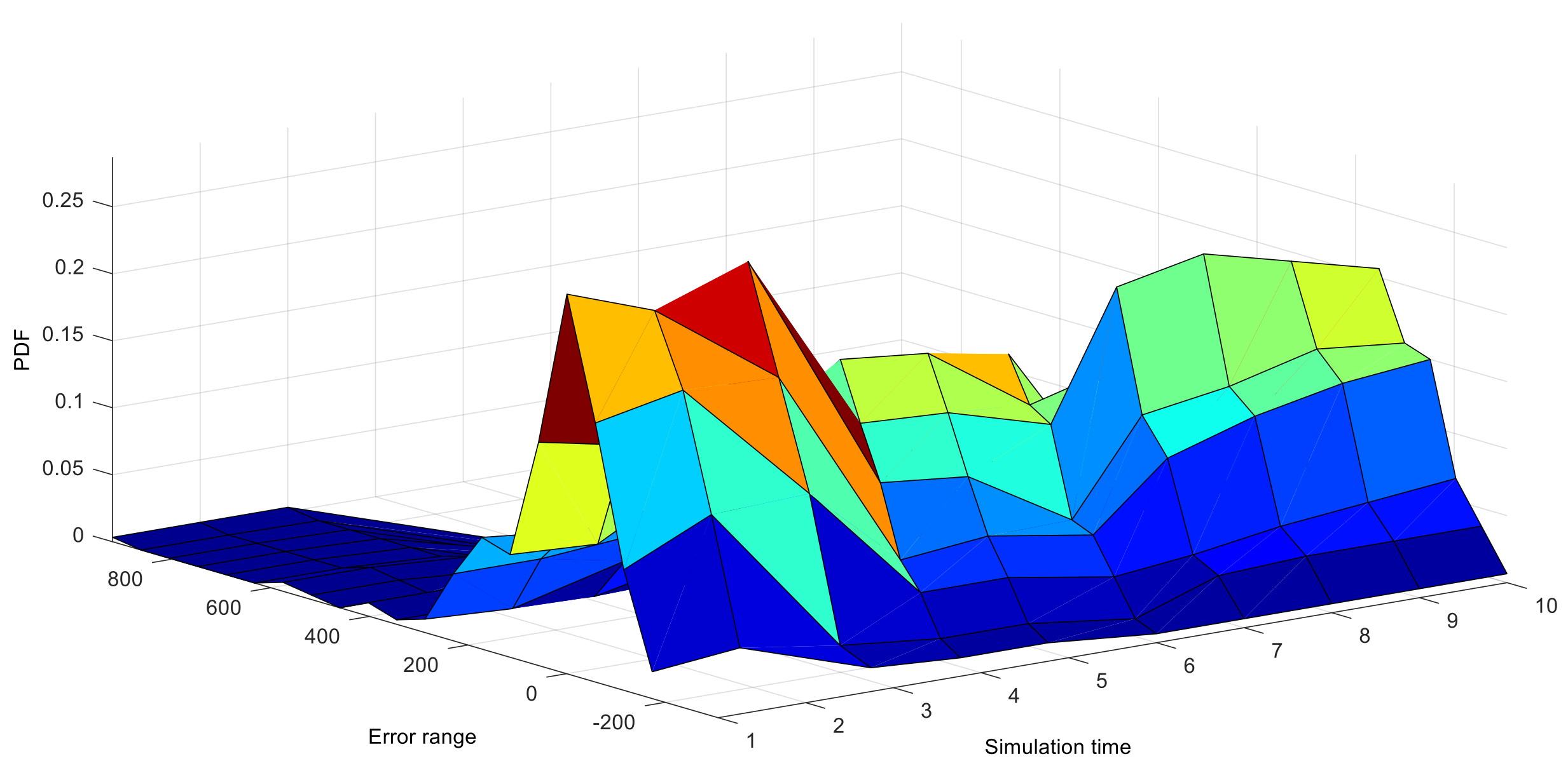
3.1. Non-Gaussian Property of Wind Power Error Sequence
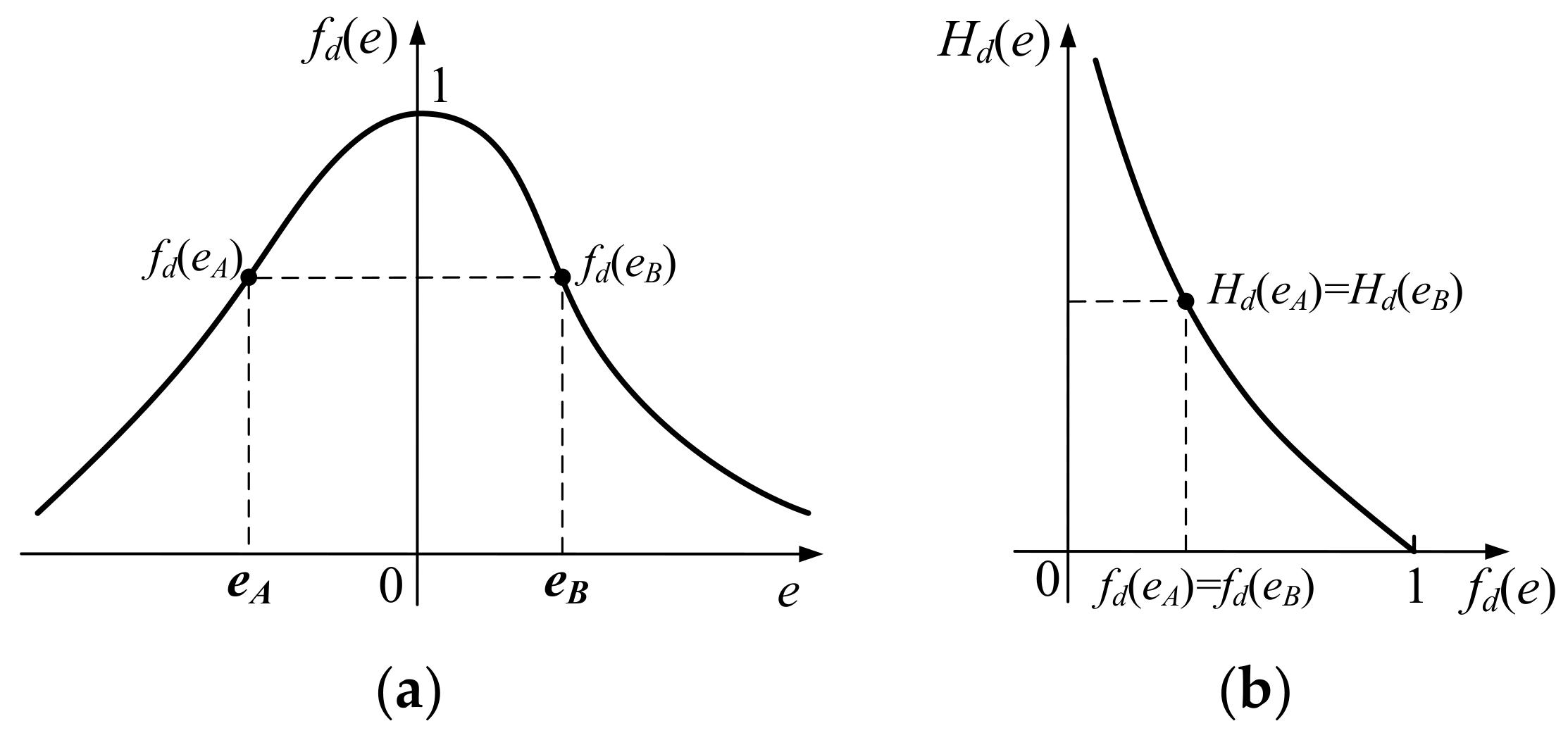
3.2. Evaluation Criterion Based on Normalized Renyi’s Quadratic Entropy
4. Simulation and Analysis
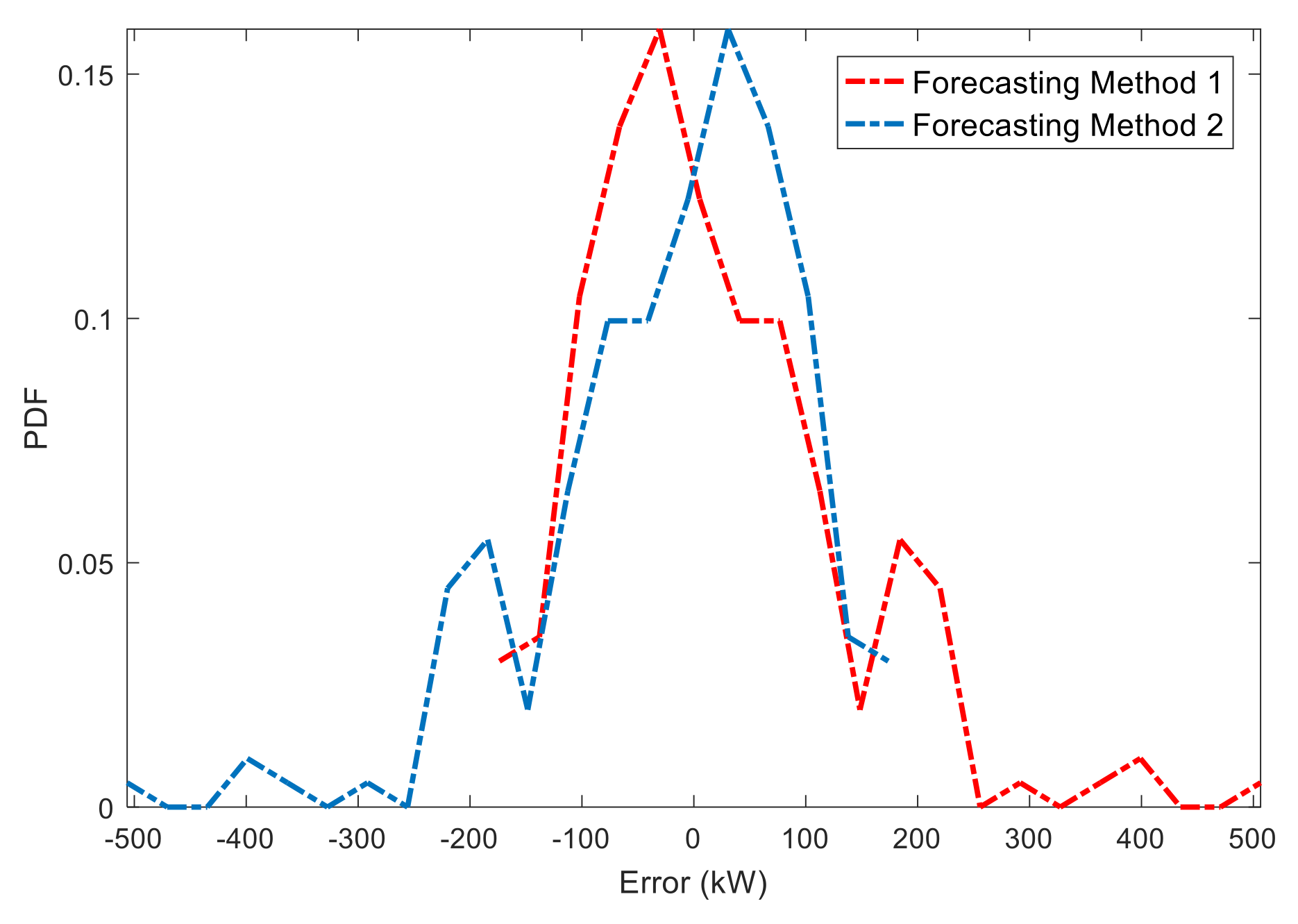
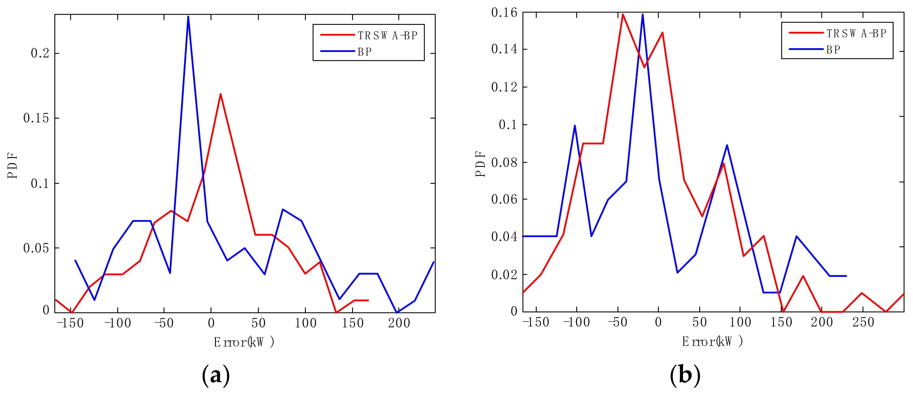
4.1. Prediction and Evaluation Based on the TRSWA-BP
4.2. Prediction Precision Based on the TRSWA-BP Combined with EMD & PSR
4.3. Training Times
5. Conclusions
Acknowledgments
Author Contributions
Conflicts of Interest
References
- Calif, R.; Schmitt, F.G.; Huang, Y. Multifractal description of wind power fluctuations using arbitrary order hilbert spectral analysis. Phys. A Stat. Mech. Appl. 2013, 392, 4106–4120. [Google Scholar] [CrossRef]
- Huang, N.E.; Shen, Z.; Long, S.R. The empirical mode decomposition and the Hilbert spectrum for nonlinear and non-stationary time series analysis. Proc. R. Soc. A 1998, 454, 903–995. [Google Scholar] [CrossRef]
- Yu, Y.L.; Li, W.; Sheng, D.R.; Chen, J.H. A hybrid short-term load forecasting method based on improved ensemble empirical mode decomposition and back propagation neural network. J. Zhejiang Univ. Sci. A 2016, 17, 101–114. [Google Scholar] [CrossRef]
- Yu, W.; Wang, M.; Feng, J. An adaptive denoising algorithm for chaotic signals based on complete ensemble empirical mode decomposition. Int. J. Inf. Commun. Technol. 2017, 11, 564–575. [Google Scholar] [CrossRef]
- Wang, S.; Zhang, N.; Wu, L.; Wang, Y. Wind speed forecasting based on the hybrid ensemble empirical mode decomposition and GA-BP neural network method. Renew. Energy 2016, 94, 629–636. [Google Scholar] [CrossRef]
- Sun, W.; Wang, Y. Short-term wind speed forecasting based on fast ensemble empirical mode decomposition, phase space reconstruction, sample entropy and improved back-propagation neural network. Energy Convers. Manag. 2018, 157, 1–12. [Google Scholar] [CrossRef]
- Wang, D.Y.; Luo, H.Y.; Grunder, O.; Lin, Y.B. Multi-step ahead wind speed forecasting using an improved wavelet neural network combining variational mode decomposition and phase space reconstruction. Renew. Energy 2017, 113, 1345–1358. [Google Scholar] [CrossRef]
- Koulaouzidis, G.; Das, S.; Cappiello, G.; Mazomenos, E.B.; Maharatna, K.; Morgan, J. A novel approach for the diagnosis of ventricular tachycardia based on phase space reconstruction of ECG. Int. J. Cardiol. 2014, 172, 31–33. [Google Scholar] [CrossRef] [PubMed][Green Version]
- Niu, M.; Gan, K.; Sun, S.; Li, F. Application of decomposition-ensemble learning paradigm with phase space reconstruction for day-ahead PM2.5 concentration forecasting. J. Environ. Manag. 2017, 196, 110–118. [Google Scholar] [CrossRef] [PubMed]
- Takens, F. Detecting strange attractors in turbulence. In Lecture Notes Mathematics; Springer: Berlin, Germany, 1981; Volume 898, pp. 366–381. [Google Scholar]
- Wolf, A.; Swift, J.B.; Swinney, H.L.; Vastano, J.A. Determining Lypunov exponents from a time series. Phys. D Nonlinear Phenom. 1985, 16, 285–317. [Google Scholar] [CrossRef]
- Guo, Z.; Chi, D.; Wu, J.; Zhang, W. A new wind speed forecasting strategy based on the chaotic time series modelling technique and the Apriori algorithm. Energy Convers. Manag. 2014, 84, 140–151. [Google Scholar] [CrossRef]
- Zhang, Y.; Lu, J.; Meng, Y. Wind power short-term forecasting based on empirical mode decomposition and chaotic phase space reconstruction. Autom. Electr. Power Syst. 2012, 36, 24–28. [Google Scholar]
- Gao, Y.; Xu, A.; Zhao, Y.; Liu, B.; Zhang, L.; Dong, L. Ultra-short-term wind power prediction based on chaos phase space reconstruction and NWP. Int. J. Control Autom. 2015, 8, 325–336. [Google Scholar] [CrossRef]
- Han, L.; Romero, C.E.; Yao, Z. Wind power forecasting based on principle component phase space reconstruction. Renew. Energy 2015, 81, 737–744. [Google Scholar] [CrossRef]
- Wang, C.; Zhang, H.; Fan, W.; Fan, X. A new wind power prediction method based on chaotic theory and Bernstein Neural Network. Energy 2016, 117, 259–271. [Google Scholar] [CrossRef]
- Safari, N.; Chung, C.Y.; Price, G.C.D. A Novel Multi-Step Short-Term Wind Power Prediction Framework Based on Chaotic Time Series Analysis and Singular Spectrum Analysis. IEEE Trans. Power Syst. 2017, 33, 590–601. [Google Scholar] [CrossRef]
- Ren, M.F.; Zhang, J.H.; Wang, H. Minimized tracking error randomness control for nonlinear multivariate and non-Gaussian systems using the generalized density evolution equation. IEEE Trans. Autom. Control 2014, 59, 2486–2490. [Google Scholar] [CrossRef]
- Song, X.; Sun, G.; Dong, S. Shannon information entropy for an infinite circular well. Phys. Lett. A 2015, 379, 1402–1408. [Google Scholar] [CrossRef]
- Macedo, D.X.; Guedes, I. Fisher information and Shannon entropy of position-dependent mass oscillators. Phys. A 2015, 434, 211–219. [Google Scholar] [CrossRef]
- Hempelmann, C.F.; Sakoglu, U.; Gurupur, V.P.; Jampana, S. An entropy-based evaluation method for knowledge bases of medical information systems. Expert Syst. Appl. 2016, 46, 262–273. [Google Scholar] [CrossRef]
- Zhao, X.; Wang, S.X. Convergence analysis of the tabu-based real-coded small-world optimization algorithm. Eng. Optim. 2014, 46, 465–486. [Google Scholar] [CrossRef]
- Wang, S.X.; Li, M.; Zhao, L.; Jin, C. Short-term wind power prediction based on improved small-world neural network. Neural Comput. Appl. 2018, 29, 1–13. [Google Scholar] [CrossRef]
- Naik, J.; Satapathy, P.; Dash, P.K. Short-term wind speed and wind power prediction using hybrid empirical mode decomposition and kernel ridge regression. Appl. Soft Comput. 2017, 8, 1–22. [Google Scholar] [CrossRef]
- Wang, J.; Zhang, W.; Li, Y.; Wang, J.; Dang, Z. Forecasting wind speed using empirical mode decomposition and Elman neural network. Appl. Soft Comput. 2014, 23, 452–459. [Google Scholar] [CrossRef]
- Kim, H.S.; Eykholt, R.; Salas, J.D. Nonlinear dynamics, delay times, and embedding windows. Phys. D 1999, 127, 48–60. [Google Scholar] [CrossRef]
- Yang, M.; Dong, J.C. Real-time prediction error analysis of wind power based on mixed Gaussian distribution model. Acta Energiae Sol. Sin. 2016, 37, 1594–1602. [Google Scholar]
- Liu, Y.; Wang, H.; Hou, C.H. UKF based nonlinear filtering using minimum entropy criterion. IEEE Trans. Signal Process. 2013, 61, 4988–4999. [Google Scholar] [CrossRef]
- Liu, Y.; Wang, H.; Guo, L. Observer-based feedback controller design for a class of stochastic systems with non-Gaussian variables. IEEE Trans. Autom. Control 2015, 60, 1445–1450. [Google Scholar] [CrossRef]


| Predictable Time Scales | 1 h | 4 h | 6 h | 24 h | |
|---|---|---|---|---|---|
| Continuous method | NMAE | 7.929% | 15.384% | 16.998% | 20.579% |
| NRMSE | 9.784% | 19.718% | 24.136% | 24.712% | |
| NRQE | 17.967 | 99.572 | 108.77 | 110.963 | |
| ARMA | NMAE | 7.117% | 15.244% | 18.729% | 23.411% |
| NRMSE | 10.258% | 20.012% | 23.881% | 27.160% | |
| NRQE | 17.845 | 94.533 | 104.686 | 123.148 | |
| SVM | NMAE | 6.090% | 9.108% | 11.153% | 14.872% |
| NRMSE | 9.488% | 10.359% | 15.025% | 18.431% | |
| NRQE | 14.333 | 25.959 | 38.65 | 88.303 | |
| BP | NMAE | 5.533% | 7.515% | 9.110% | 11.324% |
| NRMSE | 9.817% | 12.599% | 14.890% | 17.471% | |
| NRQE | 7.545 | 25.997 | 46.323 | 82.335 | |
| TRSWA-BP | NMAE | 5.218% | 6.782% | 8.080% | 10.175% |
| NRMSE | 8.144% | 10.779% | 14.033% | 17.029% | |
| NRQE | 5.945 | 20.442 | 38.422 | 64.807 | |
| Forecasting Time Scales | 1 h | 4 h | 6 h | 24 h | |
|---|---|---|---|---|---|
| TRSWA-BP and EMD (one input) | NMAE | 7.487% | 9.891% | 11.716% | 13.245% |
| NRMSE | 8.363% | 10.264% | 13.464% | 15.758% | |
| NRQE | 13.791 | 40.347 | 54.763 | 91.077 | |
| TRSWA-BP and EMD | NMAE | 6.122% | 8.325% | 9.898% | 11.652% |
| NRMSE | 7.248% | 10.029% | 12.425% | 14.780% | |
| NRQE | 2.439 | 17.967 | 23.890 | 58.461 | |
| TRSWA-BP and PSR | NMAE | 6.311% | 7.359% | 8.870% | 10.543% |
| NRMSE | 7.524% | 9.855% | 12.220% | 13.668% | |
| NRQE | 5.144 | 18.855 | 23.592 | 56.922 | |
| TRSWA-BP and EMD-based PSR | NMAE | 5.257% | 6.818% | 8.131% | 9.755% |
| NRMSE | 7.245% | 8.920% | 10.488% | 13.177% | |
| NRQE | 1.522 | 6.378 | 22.667 | 56.480 | |
© 2018 by the authors. Licensee MDPI, Basel, Switzerland. This article is an open access article distributed under the terms and conditions of the Creative Commons Attribution (CC BY) license (http://creativecommons.org/licenses/by/4.0/).
Share and Cite
Wang, S.; Zhao, X.; Li, M.; Wang, H. TRSWA-BP Neural Network for Dynamic Wind Power Forecasting Based on Entropy Evaluation. Entropy 2018, 20, 283. https://doi.org/10.3390/e20040283
Wang S, Zhao X, Li M, Wang H. TRSWA-BP Neural Network for Dynamic Wind Power Forecasting Based on Entropy Evaluation. Entropy. 2018; 20(4):283. https://doi.org/10.3390/e20040283
Chicago/Turabian StyleWang, Shuangxin, Xin Zhao, Meng Li, and Hong Wang. 2018. "TRSWA-BP Neural Network for Dynamic Wind Power Forecasting Based on Entropy Evaluation" Entropy 20, no. 4: 283. https://doi.org/10.3390/e20040283
APA StyleWang, S., Zhao, X., Li, M., & Wang, H. (2018). TRSWA-BP Neural Network for Dynamic Wind Power Forecasting Based on Entropy Evaluation. Entropy, 20(4), 283. https://doi.org/10.3390/e20040283