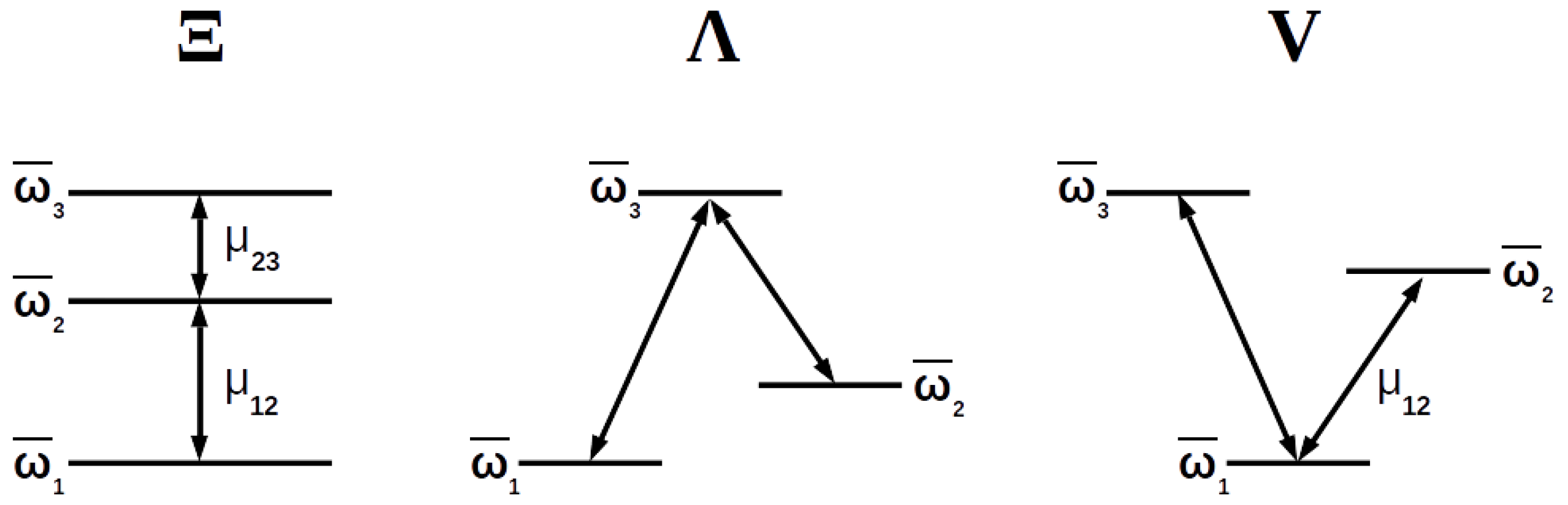
Figure 1.
Diagram showing the three possible configurations of a three-level atom according to the permitted transitions between its levels.
Figure 1.
Diagram showing the three possible configurations of a three-level atom according to the permitted transitions between its levels.
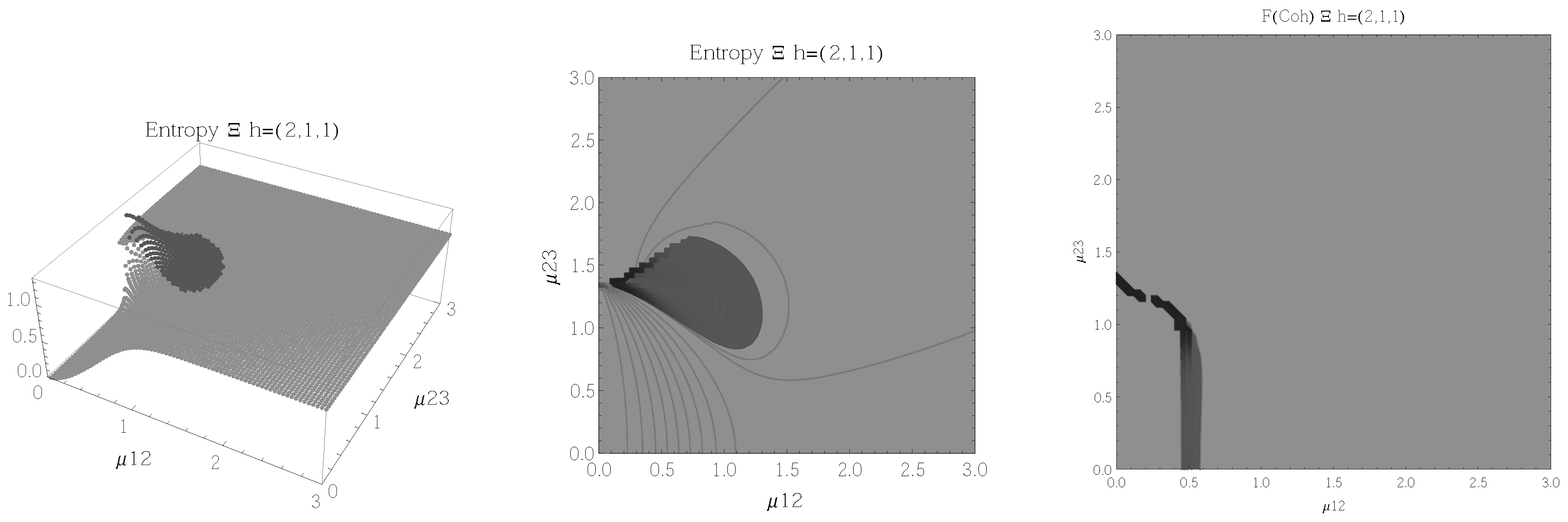
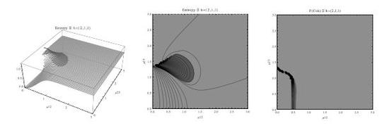
Figure 2.
(Left) 3D plot of the entropy of entanglement as a function of the coupling parameters and , the maximum value of the entropy is and the region where > 1.02 is shown in dark grey. (Center) Contour plot of the entropy of entanglement as a function of the coupling parameters and , the region where > 1.02 is shown in dark grey. (Right) Fidelity between neighbouring coherent states as a function of the coupling parameters and , dark grey region shows the fidelity’s minimum (i.e., the phase transition). All figures use , , and correspond to the configuration and the representation.
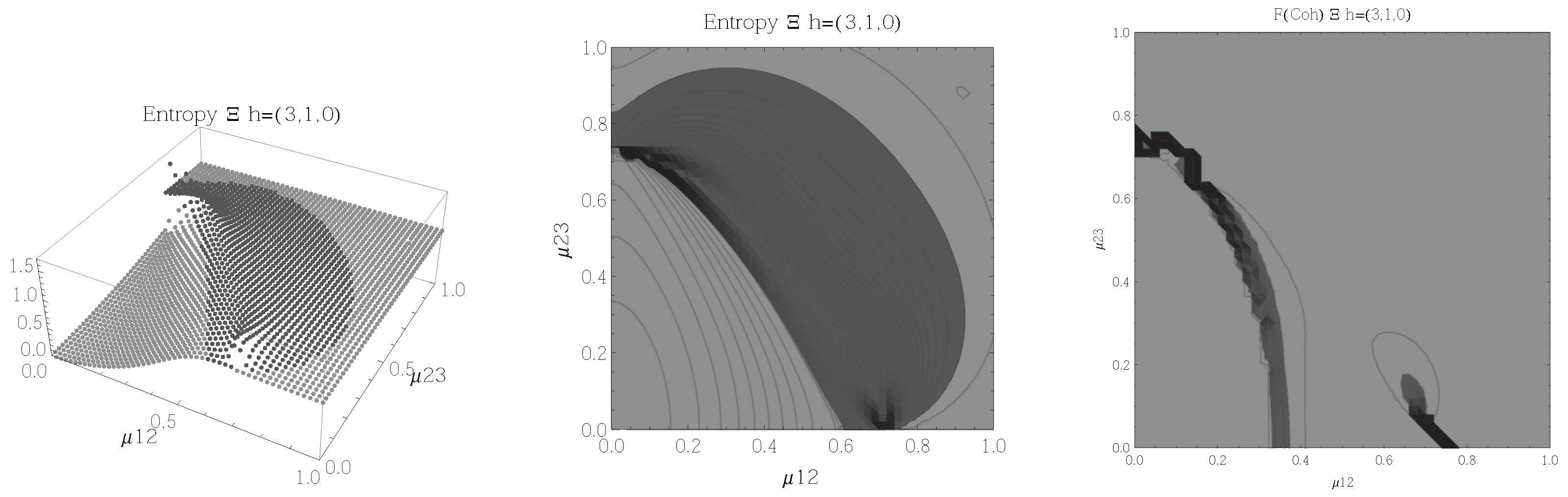
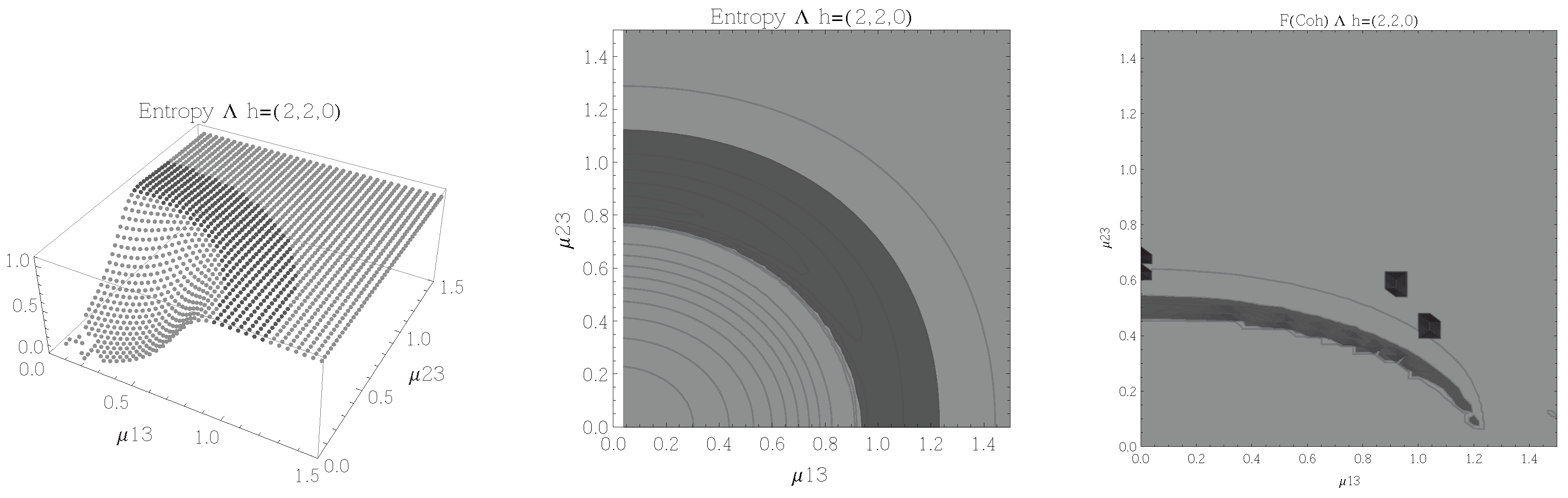
Figure 3.
(Left) 3D plot of the entropy of entanglement as a function of the coupling parameters and , the maximum value of the entropy is and the region where > 1.02 is shown in dark grey. (Center) Contour plot of the entropy of entanglement as a function of the coupling parameters and , the region where > 1.02 is shown in dark grey. (Right) Fidelity between neighbouring coherent states as a function of the coupling parameters and , dark grey region shows the fidelity’s minimum (i.e., the phase transition). All figures use , , and correspond to the configuration and the representation.
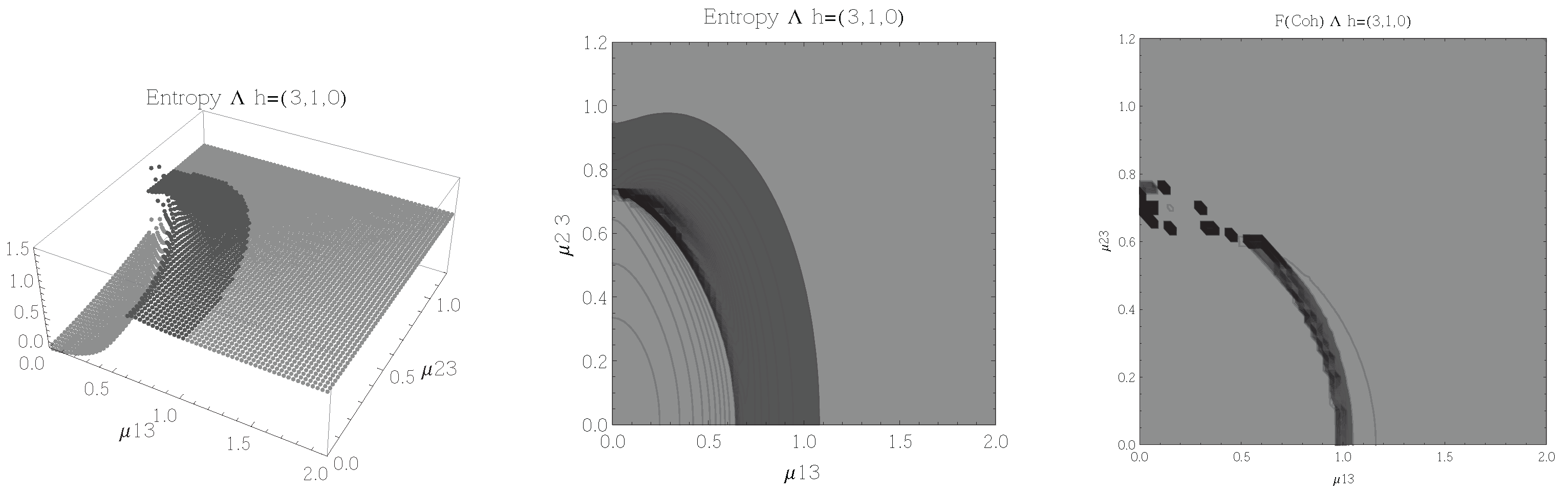
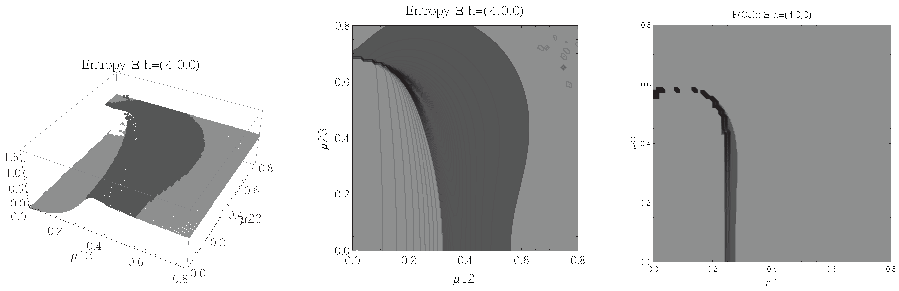
Figure 4.
(Left) 3D plot of the entropy of entanglement as a function of the coupling parameters and , the maximum value of the entropy is and the region where > 1.02 is shown in dark grey. (Center) Contour plot of the entropy of entanglement as a function of the coupling parameters and , the region where > 1.02 is shown in dark grey. (Right) Fidelity between neighbouring coherent states as a function of the coupling parameters and , dark grey region shows the fidelity’s minimum (i.e., the phase transition). All figures use , , and correspond to the configuration and the representation.
Figure 5.
(Left) 3D plot of the entropy of entanglement as a function of the coupling parameters and , the maximum value of the entropy is and the region where > 1.02 is shown in dark grey. (Center) Contour plot of the entropy of entanglement as a function of the coupling parameters and , the region where > 1.02 is shown in dark grey. (Right) Fidelity between neighbouring coherent states as a function of the coupling parameters and , dark grey region shows the fidelity’s minimum (i.e., the phase transition). All figures use , , and correspond to the configuration and the representation.
Figure 6.
(Left) 3D plot of the entropy of entanglement as a function of the coupling parameters and , the maximum value of the entropy is and the region where > 1.01 is shown in dark grey. (Center) Contour plot of the entropy of entanglement as a function of the coupling parameters and , the region where > 1.01 is shown in dark grey. (Right) Fidelity between neighbouring coherent states as a function of the coupling parameters and , dark grey region shows the fidelity’s minimum (i.e., the phase transition). All figures use , , and correspond to the configuration and the representation.
Figure 7.
(Left) 3D plot of the entropy of entanglement as a function of the coupling parameters and , the maximum value of the entropy is and the region where > 1.01 is shown in dark grey. (Center) Contour plot of the entropy of entanglement as a function of the coupling parameters and , the region where > 1.01 is shown in dark grey. (Right) Fidelity between neighbouring coherent states as a function of the coupling parameters and , dark grey region shows the fidelity’s minimum (i.e., the phase transition). All figures use , , and correspond to the configuration and the representation.
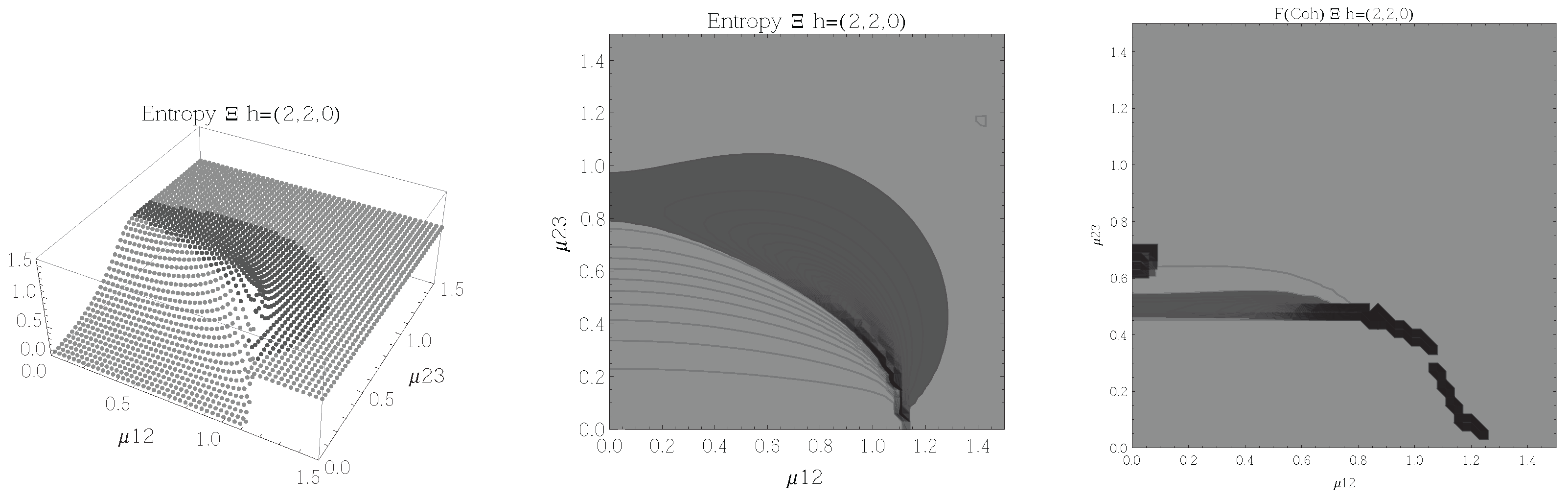
Figure 8.
(Left) 3D plot of the entropy of entanglement as a function of the coupling parameters and , the maximum value of the entropy is and the region where > 1.01 is shown in dark grey. (Center) Contour plot of the entropy of entanglement as a function of the coupling parameters and , the region where > 1.01 is shown in dark grey. (Right) Fidelity between neighbouring coherent states as a function of the coupling parameters and , dark grey region shows the fidelity’s minimum (i.e., the phase transition). All figures use , , and correspond to the configuration and the representation.
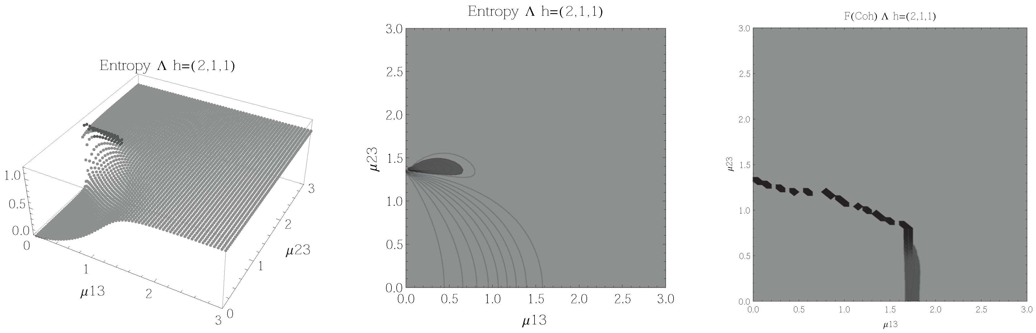
Figure 9.
(Left) 3D plot of the entropy of entanglement as a function of the coupling parameters and , the maximum value of the entropy is and the region where > 1.01 is shown in dark grey. (Center) Contour plot of the entropy of entanglement as a function of the coupling parameters and , the region where > 1.01 is shown in dark grey. (Right) Fidelity between neighbouring coherent states as a function of the coupling parameters and , dark grey region shows the fidelity’s minimum (i.e., the phase transition). All figures use , , and correspond to the configuration and the representation.
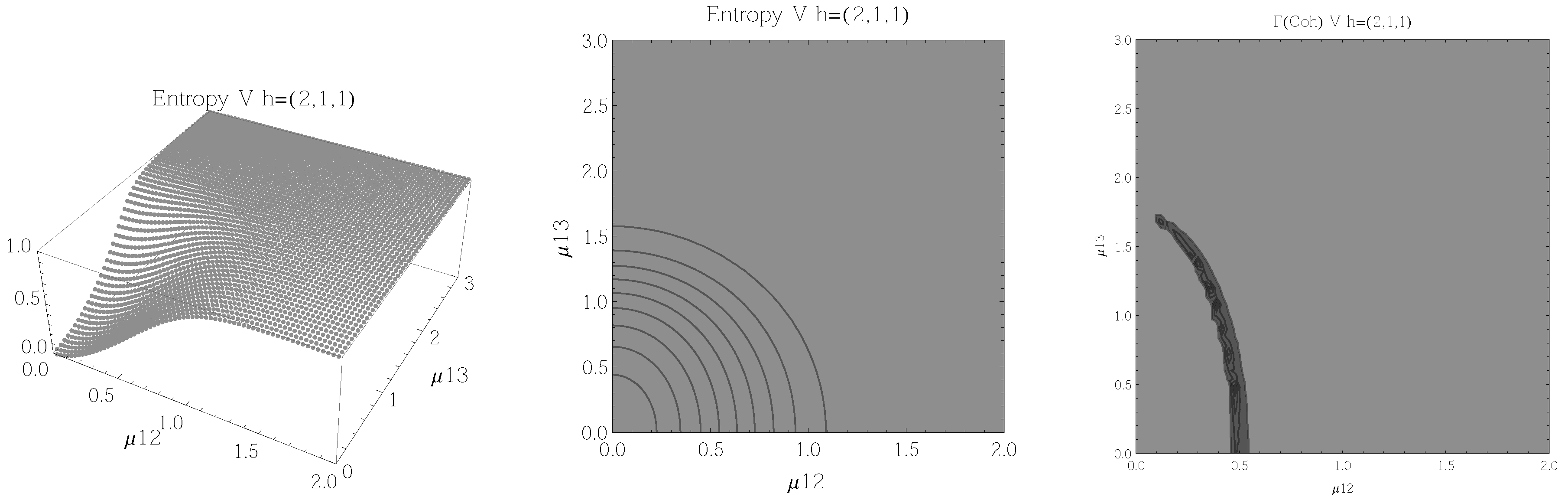
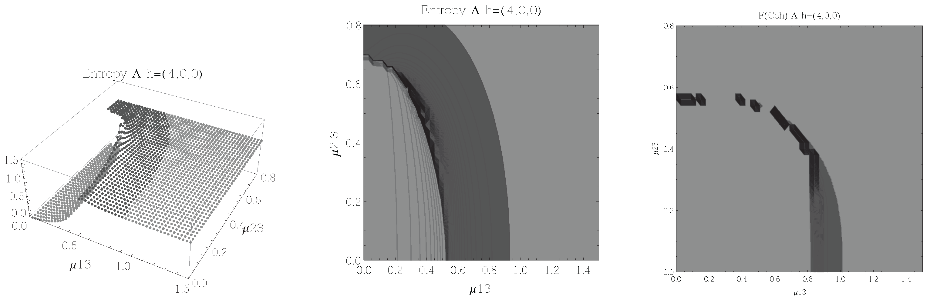
Figure 10.
(Left) 3D plot of the entropy of entanglement as a function of the coupling parameters and , the maximum value of the entropy is . (Center) Contour plot of the entropy of entanglement as a function of the coupling parameters and . (Right) Fidelity between neighbouring coherent states as a function of the coupling parameters and , dark grey region shows the fidelity’s minimum (i.e., the phase transition). All figures use , , and correspond to the V configuration and the representation.
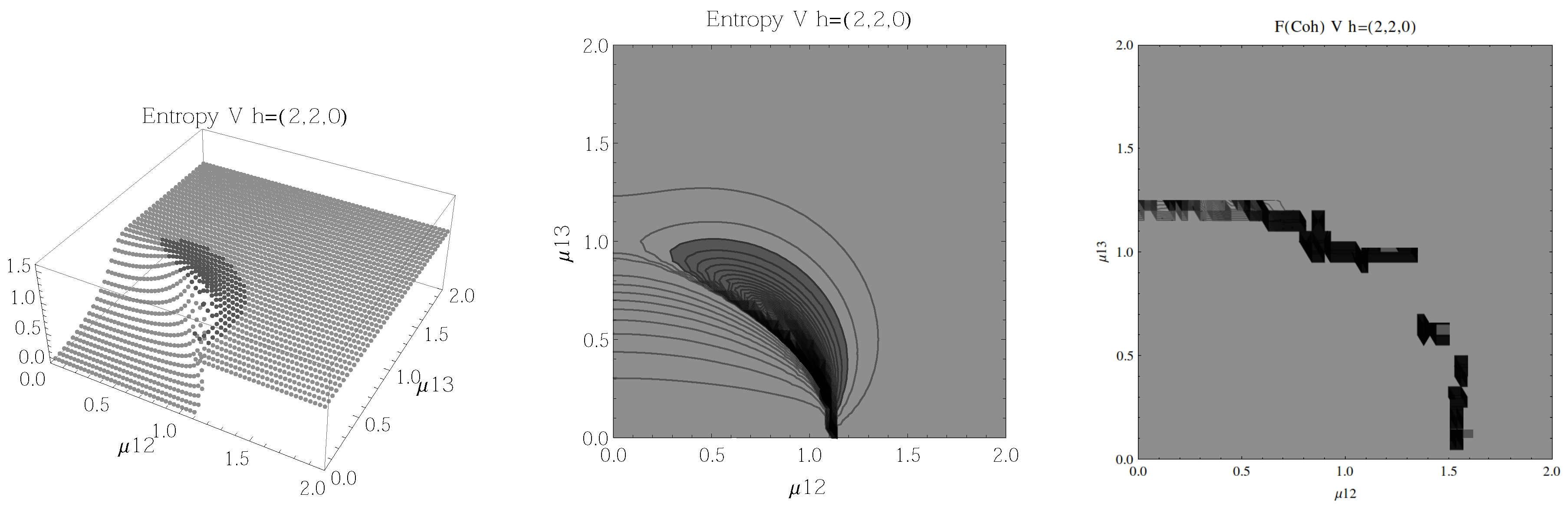
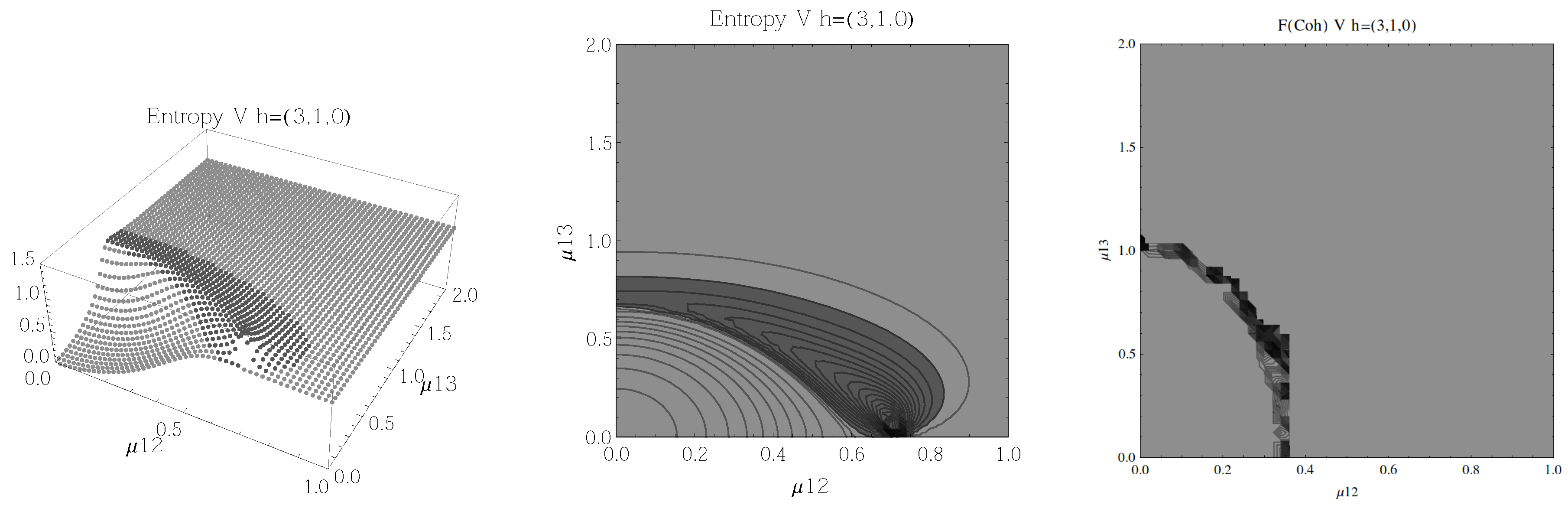
Figure 11.
(Left) 3D plot of the entropy of entanglement as a function of the coupling parameters and , the maximum value of the entropy is and the region where > 1.03 is shown in dark grey. (Center) Contour plot of the entropy of entanglement as a function of the coupling parameters and , the region where > 1.03 is shown in dark grey. (Right) Fidelity between neighbouring coherent states as a function of the coupling parameters and , dark grey region shows the fidelity’s minimum (i.e., the phase transition). All figures use , , and correspond to the V configuration and the representation.
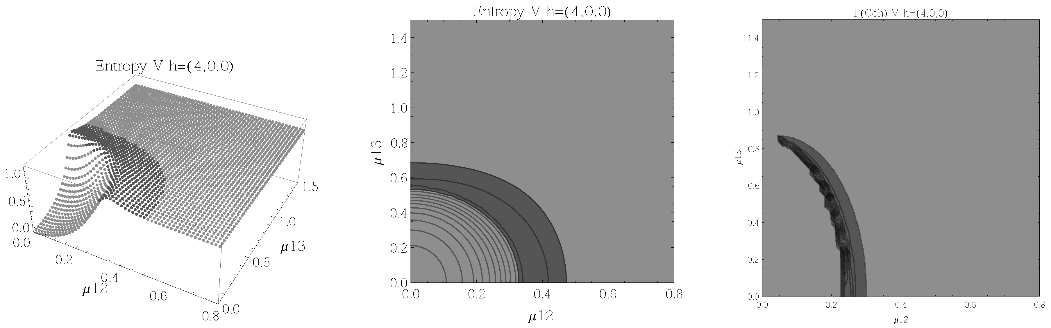
Figure 12.
(Left) 3D plot of the entropy of entanglement as a function of the coupling parameters and , the maximum value of the entropy is and the region where > 1.03 is shown in dark grey. (Center) Contour plot of the entropy of entanglement as a function of the coupling parameters and , the region where > 1.03 is shown in dark grey. (Right) Fidelity between neighbouring coherent states as a function of the coupling parameters and , dark grey region shows the fidelity’s minimum (i.e., the phase transition). All figures use , , and correspond to the V configuration and the representation.
Figure 13.
(Left) 3D plot of the entropy of entanglement as a function of the coupling parameters and , the maximum value of the entropy is and the region where > 1.03 is shown in dark grey. (Center) Contour plot of the entropy of entanglement as a function of the coupling parameters and , the region where > 1.03 is shown in dark grey. (Right) Fidelity between neighbouring coherent states as a function of the coupling parameters and , dark grey region shows the fidelity’s minimum (i.e., the phase transition). All figures use , , and correspond to the V configuration and the representation.

