1. Introduction
The knowledge of the probability distribution function (
pdf) for the velocities of systems composed of particles is an essential information to assess the nature of microscopic interactions governing such systems. A fundamental result of Statistical Mechanics concerns exactly the velocities
pdf for a collection of particles confined into a box, under the molecular chaos hypothesis, the celebrated Maxwell–Boltzmann distribution [
1]. In addition, under this assumption, collisions between particles occur randomly, and it is thus possible to anticipate that the fluctuations in the particle velocities will display a
pdf with Gaussian features. This is a consequence of the central limit theorem (
clt), once the particle velocity at a given time
t is the result of a sequence of random events (collisions), leading to a Gaussian distribution no matter how the events are distributed themselves.
These results are very robust and most of the researchers take them as a priori for data analysis. However, in nature, several systems exhibit long range inter-particle interactions, a feature which breaks one of the postulates of the molecular chaos hypothesis. In those systems, it is common to observe important deviations from Gaussian
pdf in the particle-fluctuation statistics. Tsallis and collaborators [
2] have shown that it is possible to extend the
clt to consider systems which exhibit long range or dissipative interactions by introducing the
q-Gaussian distribution [
3,
4], where the
q is an additional parameter that allows for controlling the weight of the
pdf tail. In the limit
, the Gaussian distribution is recovered, and, for
heavy or light tails—platycurtic or leptokurtic distributions, respectively—are obtained. Over the last few years, Tsallis statistics were proven to successfully describe several systems in high energy literature [
5,
6], magnetic systems [
7,
8], dissipative systems [
9] and, remarkably, several deviations from the Gaussian-like behavior were also reported in confined granular systems [
10,
11,
12].
Recently, studies with confined granular systems under shear introduced an additional problem assessing the displacement fluctuations
pdf of a given system (the displacement fluctuations correspond to the displacement deviations from the mean field). The authors have demonstrated that the
pdfs of particle fluctuations are strongly dependent on the strain increment (akin to time scale) considered in between the events [
13,
14]. The
pdf of fluctuations evolves from Gaussian-like, when large scales were considered, to heavy tail distribution for small scales, which are well described by
q-Gaussian up to five decades for the magnitude of the fluctuations of displacements [
15]. This unexpected result is indeed quite robust as it was used to verify the Tsallis–Bukman scaling law [
14,
16] which relates the
q-value obtained from fluctuation
pdf with the diffusion exponent
, related to the anomalous diffusion of the grains [
17]. Tsallis and Bukman have demonstrated that when long-range correlations are present in the system, leading to an anomalous behavior in the path drift of particles, the corresponding fluctuation
pdf exhibits heavy tails, diverging from the Gaussian-like shape. The predicted relation between these exponents, the Tsallis-Bukman scaling law
, was verified experimentally by some works [
11] but only at specific points. The first experimental verification of this law for a wide range of points was made by Combe and collaborators for a confined granular system under shearing [
14]. It is noteworthy that the measures of
q and
were completely independent, contributing to the strength of this result.
Indeed, the shear experiment with heterogeneous granular media is an ideal system to study the particle displacement fluctuations. It imposes a homogeneous deformation field over the system, but, due to the heterogeneous nature of the grains, the steric exclusion imposed by the rigidity of particles implies a wide range of magnitude to the grain fluctuations along the experiment (see Supplementary Material in [
14]). Thus, a detailed evaluation of the
pdf of grain fluctuations is essential to a proper analysis of the microscopic interactions going on in the system. In this work, we made a step further in this direction by considering a new granular system with a different size grading but applying the same methodology as in [
14]. The different grading curve employed in the present study resulted in a significant increase of the packing fraction of the system. Not surprisingly, we observed an earlier development of
shear bands during the experiments; they are zones of concentration of shear strain which are stable and can span the whole system. After a careful image analysis, we have concluded that it is possible to associate the emergence of a shear band with a sudden change in the value of the
q parameter measured as a function of the time scale. This singular behavior of
q associated with a localization event in a confined granular system, never reported before, opens a new perspective to use Statistical Mechanics tools as estimators for the emergence of shear bands or even other analogous phenomena in granular systems and heterogeneous media in general.
The paper is structured as follows: after this brief introduction, we present the experimental methodology and the details of the image analysis procedures. Next, we discuss the shear band mechanics and our results under the q-statistic viewpoint. An image analysis of the particle fluctuations considering percolation concepts is then discussed and compared with the preceding analysis. We close the paper presenting our conclusions and some perspectives for future works.
2. Materials and Methods
2.1. Experimental Setup
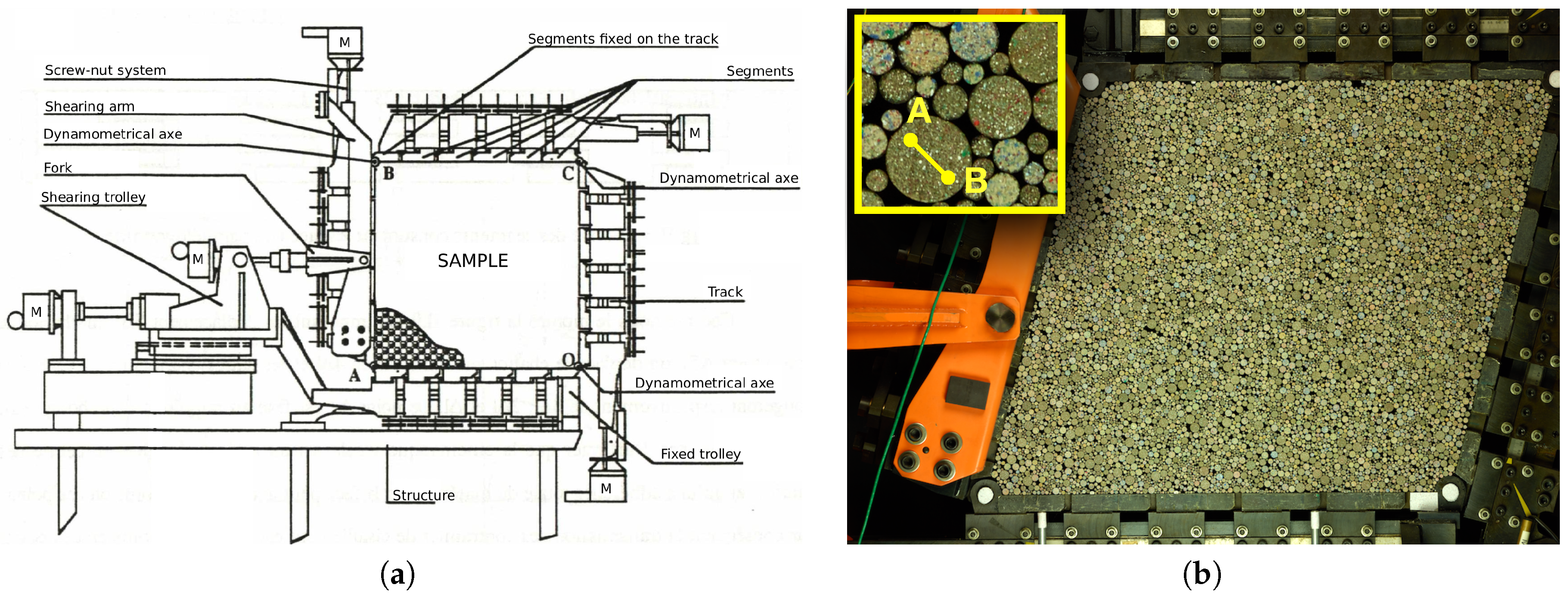
In this study, a 2D analogous granular material has been sheared with the
shear apparatus [
18,
19] at Laboratoire 3SR in Grenoble, France,
Figure 1. The
device is mainly a deformable parallelogram, which deformation is controlled by five electric motors (two synchronized for height, two for width and a last one for shear). Forces sensors installed at the corners of the parallelogram are used to compute the stress applied to the granular material. Thanks to a retro-action loop, the size of the parallelogram can be modified to impose a stress. All possible 2D strain and/or stress path can be imposed to the granular media: uniaxial compression, isotopic compression, shear, etc. This apparatus dedicated to granular materials have been used for research on various topics, such as the sensitivity of the mechanical behavior to the stress loading path [
19]; the influence of grain shape [
20] with the use of polygonal grains, mixed or not with round grains; the micro-mechanical investigations of the effect of a highly deformable intruder in a confined granular media [
21]; and the grain fluctuations in a sheared granular assembly [
14,
22].
The granular matter used in
is a 2D analogous material called Schneebeli rods [
23]. These rollers of 6 cm long, named grains hereafter, are painted on their visible face with a speckle to be followed during the test (see inset of the
Figure 1b). For all experiments presented in this paper, the granular samples were made of 11,975 grains with five different diameter sizes: 6656 grains of 3.09 mm, 2810 grains of 4.95 mm, 1459 grains of 7.09 mm, 833 grains of 9.06 mm and 217 grains of 12.14 mm. Two experimental tests were performed:
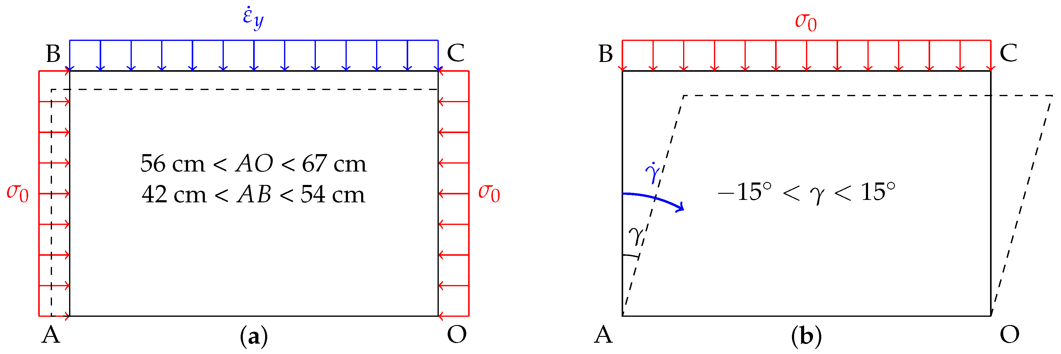
vertical compression with an imposed vertical velocity (constant imposed vertical strain rate ) with the lateral stress kept constant ( kPa)—also called biaxial vertical compression or biaxial test;
and shear test, for which parallelogram is tilted with an imposed shear rate . During the shear, the horizontal size of the sample is constant and a constant normal stress in imposed on the top of the sample. This test is also referred to as simple shear test.
The sketches of the principle of these tests are presented in
Figure 2. The imposed wall-velocity was always sufficiently low to consider that the evolution of the granular assemblies is quasi-static, which practically means that the overall mechanical response is not affected by possible adventitious “jumps” of some particles that would move dynamically; such dynamic effect can be neglected. This could be ensured considering the dimensionless
inertial number [
24,
25]
where
is the confinement pressure,
d is the mean grain diameter and
is the imposed shear rate. This inertial number measures the ratio of inertial forces of grains to imposed forces. It can also be interpreted as the time scale for grains to rearrange due to the confining stress, to the time scale for deformation by the flow. A third interpretation is the ratio of collisional stress to total stress. In terms of rheology, the so called
model discussed in [
25] allows for a clear partition of the flowing regimes as a function of
I; and it is observed and well established that
always satisfies the fact that, in a steady flow, both the internal friction
and the volume change (solid fraction) are not dependent of
I. The largest inertial number used in this paper is about
, which is well below
and allows us to safely make the assumption of quasistatic flow.
2.2. Assessment of the Full Grain-Kinematics
Digital Image Correlation (
DIC) is used to track each grain along all the photographs. This technique was firstly suggested in [
26] and largely developed since the beginning of the century to provide kinematics fields from images (displacement, strain, accelerations, etc.) in continuous materials (metals, polymers, concrete, etc.). In our case, the goal is not to determine strain fields from
local mean displacements of an amount of grains but to follow the motion of each individual grain (supposed to be rigid). The quantities to be determined are the displacement (components
and
) and the rotation (
) relative to the first image. This is very different from classical applications of
DIC as grains could move erratically and significantly between two successive images (especially in case of grain rearrangements), so the variations
,
and
are not necessarily small or continuous in space. Specific tools are thus needed to follow individual grains—without losing any of them and with high precision of the tracked motions—in granular materials. The tool
Tracker [
27] has been developed exactly for this purpose.
The basis of the
DIC is to find the displacement of a pattern (subset of the reference image) on all images. The best pixel position is chosen with the best correlation coefficient
, which is the
zero-mean normalized cross-correlation (ZNCC) coefficient. First, all positions and rotations are tested at pixels scale in a ranged neighborhood of last known position of the grain by assuming that grains do not move a lot during the 5 s between successive photographs, typically around 1 pixel. The recognition is supposed to be correct if
is not under a given threshold (
); otherwise, the neighborhood ranges are enlarged. At this point, the pixel position is given by integers and the rotation is
quantized due to the discrete nature of the signal. To refine the positions and rotations at a sub-pixel resolution, the signal from second image is made continuous thanks to a bi-cubic interpolation of the gray levels, and the best values of (
,
,
) are found with a sub-pixel precision by minimizing
; Powell’s conjugate direction method [
28] is used to this end.
For Schneebeli rods, circular patterns centered on grains are used; their diameters are 80% of the tracked grain diameters to avoid local deformations due to contact to be in the correlation area. Localization of already identified grains are also used to reduce the search area and make the first stage of the correlation faster. After the grain tracking, the positions are corrected to account for image distortion with the Brown–Conrady model [
29]. The scaling of images is done on the first images with two points whose distance is known at the beginning of the test. The movement of the camera is corrected with the help of a set of points which are not supposed to move on the frame of the
apparatus and covered by a speckle. Grains with an insufficient correlation coefficient (under 0.7) are removed from the data by checking that they remain very few.
In all photographs, it is also possible to measure the mean stream, following the four corners of the , which were also painted with a speckle. Finally, each grain comes with an actual motion and the affine motion it would have if it obeys a homogeneous deformation gradient.
2.3. Accuracy of Tracked Kinematics
Accuracies of measurements of grain kinematics must take into account the full measurement chain, from the camera lens to the
DIC software. In particular, but not exclusively, inaccuracies come from the lens distortion, the Charge-Coupled Device (CCD) sensor of the camera (that blur the image to avoid Moiré effects), the algorithm used for demosaicing the image (Bayer matrix), the quality of the speckle painted on each grain and the degree of complexity of the function of interpolation of the image (to obtain sub-pixel measurements). A way to assess a reliable measurement of the error on the kinematics is to grab every source of error together. Considering that the grains are perfectly rigid, any internal distance should remain constant whatever the strain/stress path imposed to the granular sample, i.e., whatever the displacements and the rotations of the grains. To test this, the two extremities
A and
B of several segments are tracked together with the translation and rotation of all grains in the sample; see inset in
Figure 1. Considering the first digital image as a reference, the initial lengths
of the segments
i should not change for the other images. Therefore, the variations of length
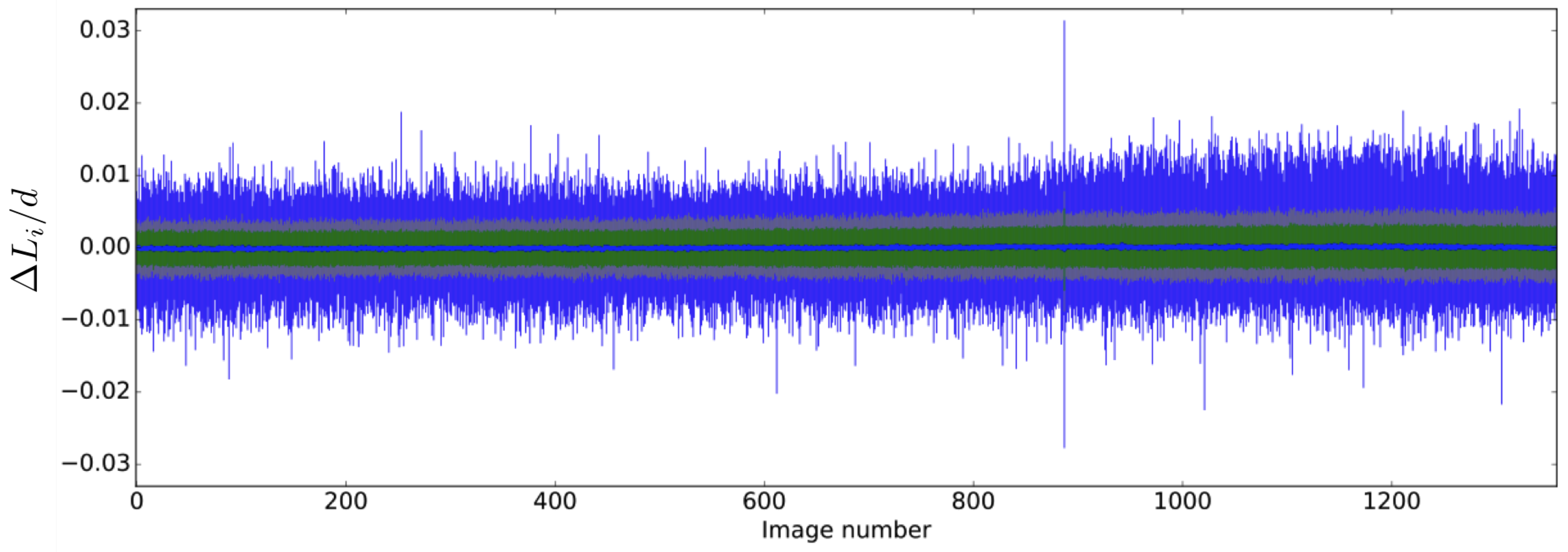
as a function of the
Nth image provides an estimation of the kinematics error. The average errors
for each photograph were computed from 434 segments over more than 1300 photographs that have been shot during a shear test (
Figure 3) for which the maximum grain displacement was about 10 cm.
In this example, it is possible to observe a standard deviation of in the range of the mean-diameter d with a nearly null average error. The distribution of errors follows a Gaussian function that remains nearly the same for all photographs. The maximum error is on the order of ∼1% of the mean diameter, and it goes exceptionally to (this appended actually only one time because of an unintentional kick in the camera). In view of the number of grains in each photograph, this high level of accuracy was made possible thanks to a 80 MPixels digital Camera and a particular care to circumvent the possible sources of inaccuracy (correction of lens distortion and camera parallax, check of pattern quality, choice of the debayering algorithm, careful choice of the interpolation function for sub-pixel gauging, uniform lighting, etc).
2.4. Fluctuation of the Displacements
In a granular packing, a grain trajectory does not necessarily follow the homogeneous displacement field imposed at the macroscopic level (sample scale). This is due to geometrical constraints at the grain scale (steric exclusion)—grains are not able to displace as continuum mechanics dictates that they should. The fluctuation of displacement can be defined as the difference between the actual displacement —measured with DIC—and the displacement that the same point would have if it had obeyed a homogeneous strain (equal to the imposed macroscopic one) .
It is useful to introduce a dimensionless fluctuation
v as a ratio between the physical displacement fluctuation and the typical length
where
is a homogeneous macroscopic strain and
d is the mean diameter of the grains:
Depending on the test, can be either an increment of shear strain (variation of the tilt angle) or the vertical strain . The apparatus was designed so that the sample is disposed vertically; that is to say, the gravity acts on the y component of our images which could introduce a bias in the fluctuations. To avoid this effect as much as possible, it has been chosen to study mainly the x coordinate of the fluctuations, .
2.5. Local Strains
A local two-dimensional strain tensor can be defined using the Delaunay triangulation of grain centers, where displacements are known. A mean strain tensor for each triangle is given thanks to the Stokes theorem as the contour integral:
where
is the displacement vector at the boundary of the triangle,
the outgoing normal vector,
S the triangle surface and
ℓ the contour length [
19]. From the tensor
, it is possible to use all the components to highlight local/microscopic strains. However, a convenient way to study the strain localization in granular material is basically to focus on two invariants of the strain: the volumetric strain
or the shear intensity
, where
are the two eigenvalues of
. It should be noticed that the chosen sign convention is such that a strain component is positive when lengths reduce.
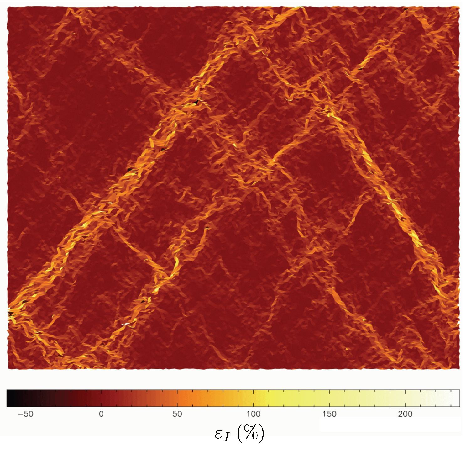
Figure 4 gives an example of a shear band network in a granular material subjected to a biaxial compression.
Hereafter, for a sake of simplicity, strain localization will generally be illustrated by means of which has the advantage of being always positive or equal to zero.
3. Shear Band Mechanism
When plasticity occurs in a heterogeneous material submitted to a deviatoric loading, strains can concentrate in specific zones, and their locations are generally impossible to predict. These specific zones are zones where the imposed strains on the sample (macroscopic scale) concentrate locally by making patterns in the form of bands (see
Figure 4). These bands are termed
shear bands since they are the places where the microscopic shear strain over-expresses, the rest of the volume being weakly deformed compared with the mean strain. For dense granular material, it has been shown that strain localization is a key mechanism of plasticity evolution. These shear bands are experimentally observed either for sand [
30], for analogous granular material like
Schneebeli materials [
19,
31] and also for virtual granular models like those used in DEM (Discrete Element Model) [
21], or double scale FEM × DEM (Finite Element Model at macroscopic scale, and Discrete Element Model at the microscopic scale) [
32]. It might be important to stress that shear bands are steady with fixed positions and orientation, but they can appear for different shear strain
during the loading; they, however, never decline for monotonic loading. The emergence of shear bands can be pictured by keeping in mind that the zones of concentrated shear-strain form straight bands (typically 10 to 20 particle diameters in width), they can be multiple and they can be reflected at the sample boundaries (like in the
Figure 4 where shearbands reflect on the rigid boundaries). For high shear strain levels, the map of strain anisotropy, as observable in
Figure 4 and
Figure 5 gives the false impression of locally varying inhomogeneities, but they are actually several straight shear bands having the same inclination (or reflected inclination) that intersect one another. When a granular material is submitted to an external loading path, shear bands do not appear instantaneously. Whereas the orientation of shearband can be more or less predicted by the Rankine’s earth-pressure theory, during the past 50 years, many research works tried to explore and to understand how shear bands appear and develop. Very recently, new progress in the
DIC technique and with the improvement of very high resolution of digital cameras helps to observe that shear banding can occurs well before reaching the maximum strength of the granular assembly [
33]. However, important questions remain: why and how do the shear bands appear?
We focus here on the so-called vertical biaxial compression test. An imposed vertical strain increases with a constant rate all along the compression. This strain rate is such that the sample deforms in a quasi-static regime. At the end of the test, the macroscopic vertical strain can reach
or more. After a given macroscopic vertical strain
(typically 2%), a network of oblique shear bands can already be observed. Strain localized zones can be plotted and identified for a given imposed macroscopic strain increment
using various local indicators like the increments of the second invariant
(shear intensity). Strain field of
have been computed for different macroscopic strain increments
from a macroscopic strain-level for which the shear bands have already started to develop,
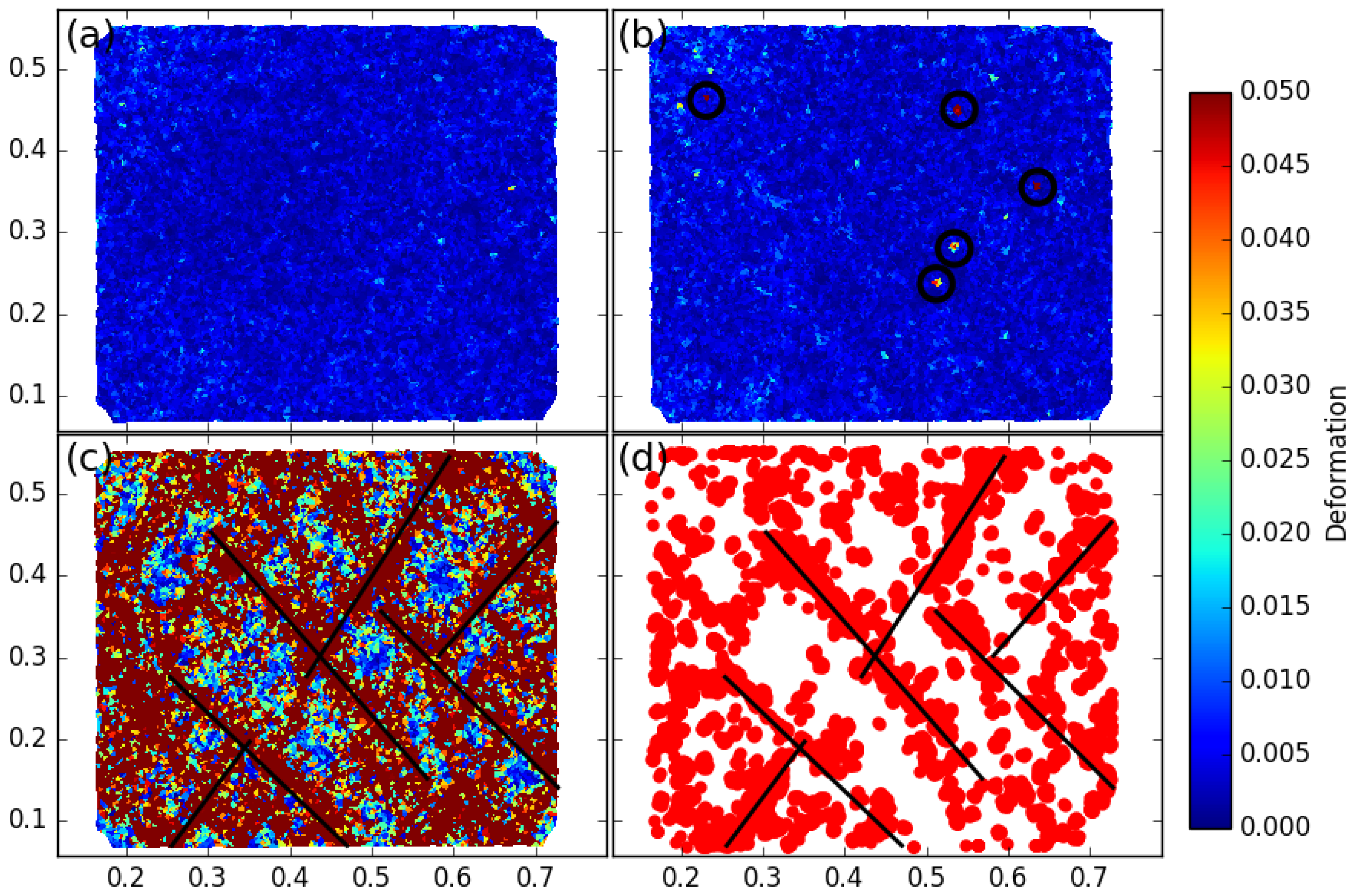
. The first striking point is that, when plotting the map of
for a very small increment
, the shear bands are not apparent, as shown in
Figure 5a. However, sometimes, for such very low strain increments, some concentrated local strain peaks occur (
Figure 5b). It is possible to observe fully developed shear bands only for increments of strain greater or equal to 2%, as shown in
Figure 5c.
It is observed in
Figure 5c that the rare local peaks of
(computed for the low strain increment,
Figure 5d) aggregated in the course of time reconstruct the picture of shear bands. Thus, the concept of shear bands seem to be relevant only when a sufficient macroscopic increment of strain is reached. This separates two regimes in terms of
: when the macroscopic increment of strain is small, no extended localization zone appears except some very local microscopic events with no manifest correlation in space; when the macroscopic strain reaches a sufficiently large value, the imposed macroscopic strain localizes into shear bands that percolate throughout the granular sample.


