The Interaction Analysis between the Sympathetic and Parasympathetic Systems in CHF by Using Transfer Entropy Method

Abstract
1. Introduction
2. Materials and Methods
2.1. Data
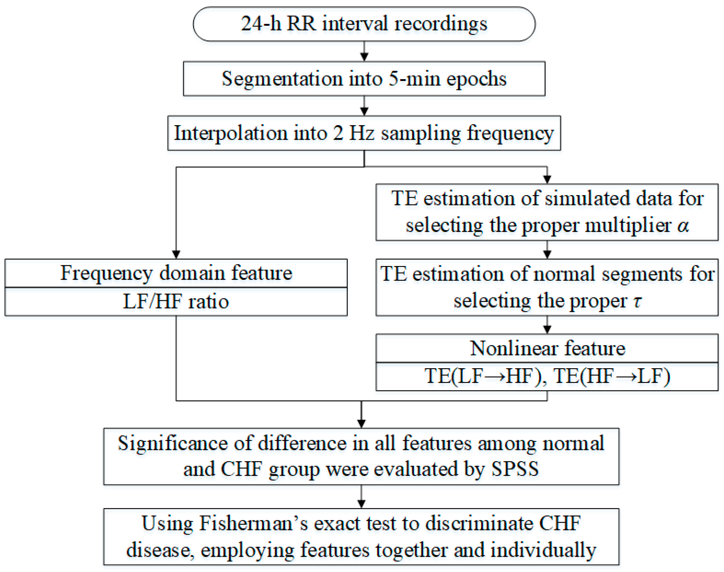
2.2. Feature Extraction
2.2.1. LF/HF Ratio
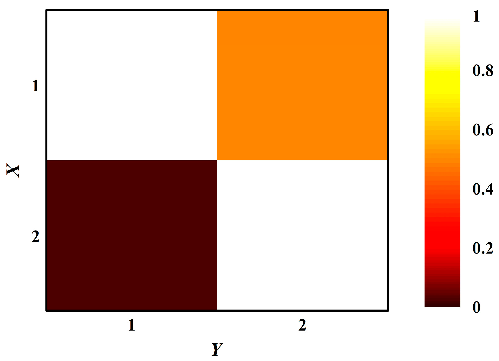
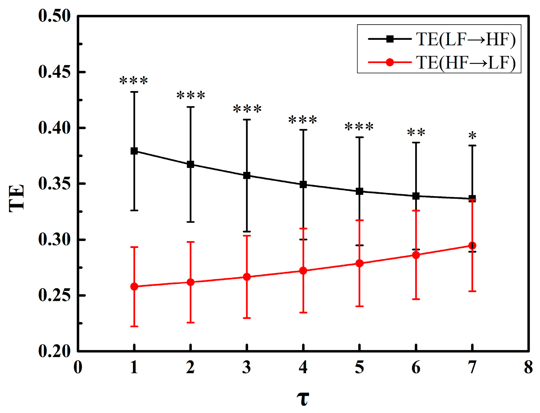
2.2.2. TE
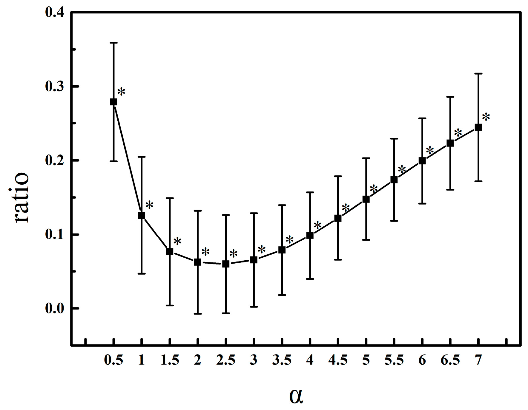
2.2.3. Simulation
2.3. Performance Evaluation
3. Results
3.1. Parameter Selection
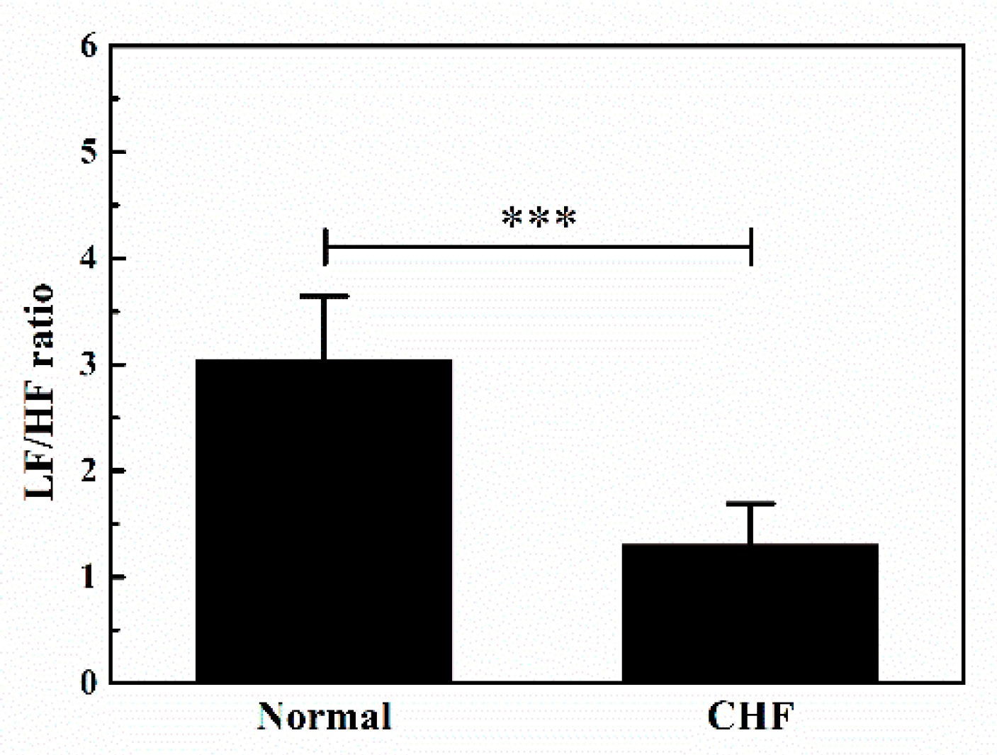
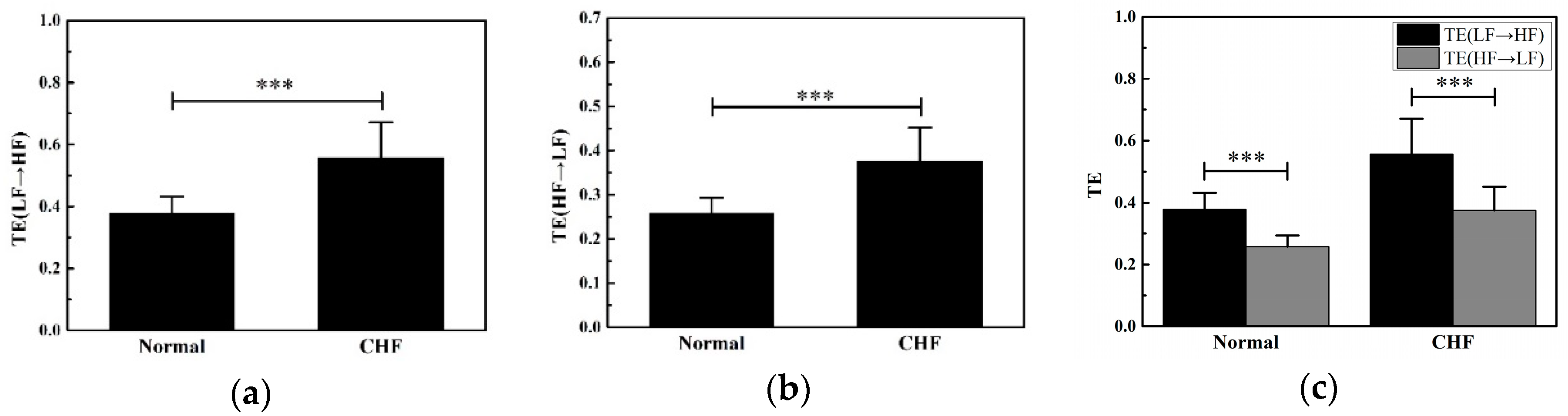
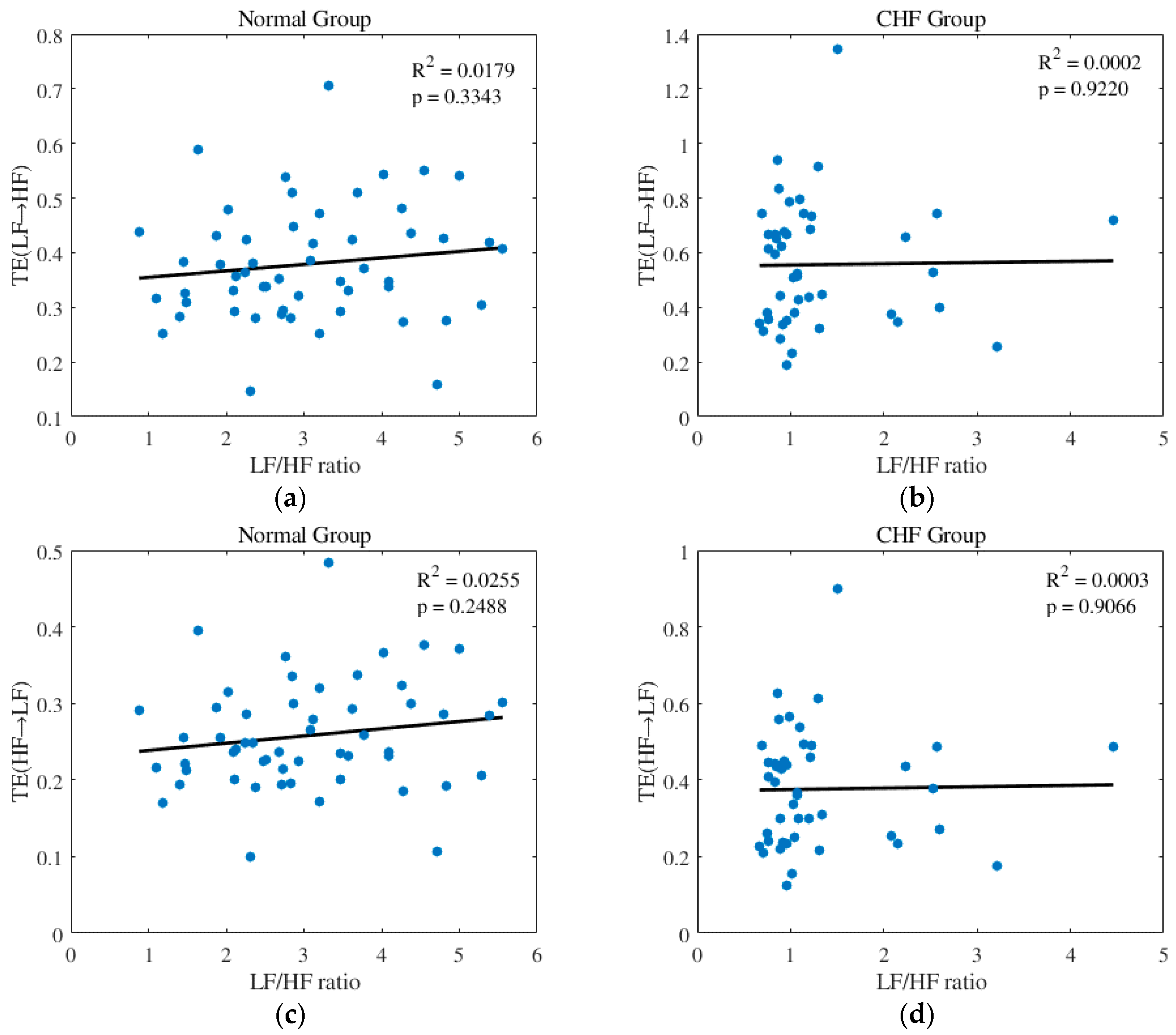
3.2. Features Analysis
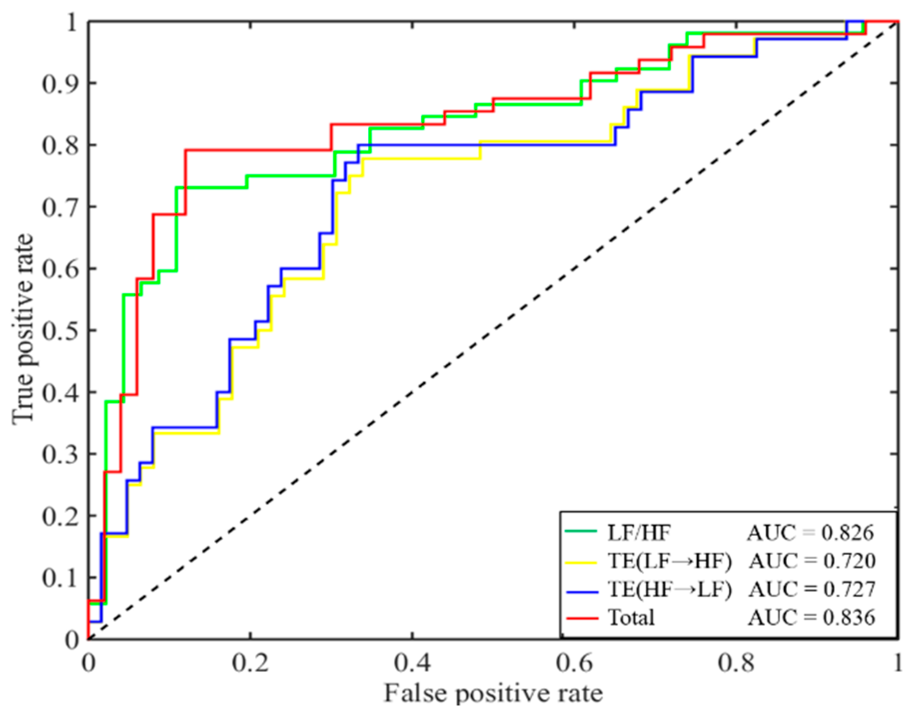
3.3. Classification
4. Discussion
4.1. Comparison and Summary
4.2. Physiological Significance
4.3. Parameter Discussion
5. Conclusions
Author Contributions
Funding
Conflicts of Interest
References
- Keith, J.D. Congestive heart failure. Pediatrics 1956, 18, 491–500. [Google Scholar] [PubMed]
- Nolan, J.; Batin, P.D.; Andrews, R.; Lindsay, S.J.; Brooksby, P.; Mullen, M.; Baig, W.; Flapan, A.D.; Cowley, A.; Prescott, R.J.; et al. Prospective study of heart rate variability and mortality in chronic heart failure: Results of the United Kingdom heart failure evaluation and assessment of risk trial (UK-heart). Circulation 1998, 98, 1510–1516. [Google Scholar] [CrossRef] [PubMed]
- Variability, H.R. Heart rate variability: Standards of measurement, physiological interpretation and clinical use. task force of the european society of cardiology and the north american society of pacing and electrophysiology. Circulation 1996, 93, 1043–1065. [Google Scholar]
- Rao, A.M.; Ryoo, H.C.; Akin, A.; Sun, H.H. Classification of Heart Rate Variability (HRV) Parameters by Receiver Operating Characteristics (ROC); IEEE: New York, NY, USA, 2002. [Google Scholar]
- Ponikowski, P.; Anker, S.D.; Chua, T.P.; Szelemej, R.; Piepoli, M.; Adamopoulos, S.; Webb-Peploe, K.; Harrington, D.; Banasiak, W.; Wrabec, K.; et al. Depressed heart rate variability as an independent predictor of death in chronic congestive heart failure secondary to ischemic or idiopathic dilated cardiomyopathy. Am. J. Cardiol. 1997, 79, 1645–1650. [Google Scholar] [CrossRef]
- Piccirillo, G.; Magri, D.; Naso, C.; di Carlo, S.; Moise, A.; de Laurentis, T.; Torrini, A.; Matera, S.; Nocco, M. Factors influencing heart rate variability power spectral analysis during controlled breathing in patients with chronic heart failure or hypertension and in healthy normotensive subjects. Clin. Sci. 2004, 107, 183–190. [Google Scholar] [CrossRef] [PubMed]
- Poon, C.-S.; Merrill, C.K. Decrease of cardiac chaos in congestive heart failure. Nature 1997, 389, 492–495. [Google Scholar] [CrossRef] [PubMed]
- Makikallio, T.H.; Huikuri, H.V.; Hintze, U.; Videbaek, J.; Mitrani, R.D.; Castellanos, A.; Myerburg, R.J.; Møller, M.; DIAMOND Study Group. Fractal analysis and time- and frequency-domain measures of heart rate variability as predictors of mortality in patients with heart failure. Am. J. Cardiol. 2001, 87, 178–182. [Google Scholar] [CrossRef]
- Liu, G.; Wang, L.; Wang, Q.; Zhou, G.; Wang, Y.; Jiang, Q. A new approach to detect congestive heart failure using short-term heart rate variability measures. PLoS ONE 2014, 9, e93399. [Google Scholar] [CrossRef] [PubMed]
- Mudd, J.O.; Kass, D.A. Tackling heart failure in the twenty-first century. Nature 2008, 451, 919–928. [Google Scholar] [CrossRef] [PubMed]
- Ajiki, K.; Murakawa, Y.; Yanagisawa-Miwa, A.; Usui, M.; Yamashita, T.; Oikawa, N.; Inoue, H. Autonomic nervous system activity in idiopathic dilated cardiomyopathy and in hypertrophic cardiomyopathy. Am. J. Cardiol. 1993, 71, 1316–1320. [Google Scholar] [CrossRef]
- Li, Y.; Pan, W.; Li, K.; Jiang, Q.; Liu, G.Z. Sliding trend fuzzy approximate entropy as a novel descriptor of heart rate variability in obstructive sleep apnea. IEEE J. Biomed. Health Inform. 2018. [Google Scholar] [CrossRef] [PubMed]
- Schreiber, T. Measuring information transfer. Phys. Rev. Lett. 2000, 85, 461–464. [Google Scholar] [CrossRef] [PubMed]
- Faes, L.; Nollo, G.; Porta, A. Compensated transfer entropy as a tool for reliably estimating information transfer in physiological time series. Entropy 2013, 15, 198–219. [Google Scholar] [CrossRef]
- Olshansky, B.; Sabbah, H.N.; Hauptman, P.J.; Colucci, W.S. Parasympathetic nervous system and heart failure—Pathophysiology and potential implications for therapy. Circulation 2008, 118, 863–871. [Google Scholar] [CrossRef] [PubMed]
- Faes, L.; Nollo, G.; Porta, A. Information domain approach to the investigation of cardio-vascular, cardio-pulmonary, and vasculo-pulmonary causal couplings. Front. Physiol. 2011, 2, 2011. [Google Scholar] [CrossRef] [PubMed]
- Marzbanrad, F.; Kimura, Y.; Palaniswami, M.; Khandoker, A.H. Quantifying the interactions between maternal and fetal heart rates by transfer entropy. PLoS ONE 2015, 10, e0145672. [Google Scholar] [CrossRef] [PubMed]
- Katura, T.; Tanaka, N.; Obata, A.; Sato, H.; Maki, A. Quantitative evaluation of interrelations between spontaneous low-frequency oscillations in cerebral hemodynamics and systemic cardiovascular dynamics. Neuroimage 2006, 31, 1592–1600. [Google Scholar] [CrossRef] [PubMed]
- Porta, A.; Marchi, A.; Bari, V.; de Maria, B.; Esler, M.; Lambert, E.; Baumert, M. Assessing the strength of cardiac and sympathetic baroreflex controls via transfer entropy during orthostatic challenge. Philos. Trans. R. Soc. Math. Phys. Eng. Sci. 2017, 375. [Google Scholar] [CrossRef] [PubMed]
- Zheng, L.; Pan, W.; Li, Y.; Luo, D.; Wang, Q.; Liu, G. Use of mutual information and transfer entropy to assess interaction between parasympathetic and sympathetic activities of nervous system from HRV. Entropy 2017, 19, 489. [Google Scholar] [CrossRef]
- Berntson, G.G.; Bigger, J.T., Jr.; Eckberg, D.L.; Grossman, P.; Kaufmann, P.G.; Malik, M.; Nagaraja, H.N.; Porges, S.W.; Saul, J.P.; Stone, P.H.; et al. Heart rate variability: Origins, methods, and interpretive caveats. Psychophysiology 1997, 34, 623–648. [Google Scholar] [CrossRef] [PubMed]
- Montano, N.; Ruscone, T.G.; Porta, A.; Lombardi, F.; Pagani, M.; Malliani, A. Power spectrum analysis of heart rate variability to assess the changes in sympathovagal balance during graded orthostatic tilt. Circulation 1994, 90, 1826–1831. [Google Scholar] [CrossRef] [PubMed]
- Malliani, A.; Pagani, M.; Lombardi, F.; Cerutti, S. Cardiovascular neural regulation explored in the frequency domain. Circulation 1991, 84, 482–492. [Google Scholar] [CrossRef] [PubMed]
- Binkley, P.F.; Nunziata, E.; Haas, G.J.; Nelson, S.D.; Cody, R.J. Parasympathetic withdrawal is an integral component of autonomic imbalance in congestive heart failure: Demonstration in human subjects and verification in a paced canine model of ventricular failure. J. Am. Coll. Cardiol. 1991, 18, 464–472. [Google Scholar] [CrossRef]
- Baim, D.S.; Colucci, W.S.; Monrad, E.S.; Smith, H.S.; Wright, R.F.; Lanoue, A.; Gauthier, D.F.; Ransil, B.J.; Grossman, W.; Braunwald, E.; et al. Survival of patients with severe congestive heart failure treated with oral milrinone. J. Am. Coll. Cardiol. 1986, 7, 661–670. [Google Scholar] [CrossRef]
- Chen, W.H.; Zheng, L.R.; Li, K.Y.; Wang, Q.; Liu, G.Z.; Jiang, Q. A novel and effective method for congestive heart failure detection and quantification using dynamic heart rate variability measurement. PLoS ONE 2016, 11, e0165304. [Google Scholar] [CrossRef] [PubMed]
- Pagani, M.; Lombardi, F.; Guzzetti, S.; Rimoldi, O.; Furlan, R.; Pizzinelli, P.; Sandrone, G.; Malfatto, G.; Dell’Orto, S.; Piccaluga, E. Power spectral analysis of heart rate and arterial pressure variabilities as a marker of sympatho-vagal interaction in man and conscious dog. Circ. Res. 1986, 59, 178–193. [Google Scholar] [CrossRef] [PubMed]
- Lee, J.; Nemati, S.; Silva, I.; Edwards, B.A.; Butler, J.P.; Malhotra, A. Transfer entropy estimation and directional coupling change detection in biomedical time series. BioMed. Eng. Online 2012, 11, 19. [Google Scholar] [CrossRef] [PubMed]
- Montalto, A.; Faes, L.; Marinazzo, D. MuTE: A MATLAB toolbox to compare established and novel estimators of the multivariate transfer entropy. PLoS ONE 2014, 9, e109462. [Google Scholar] [CrossRef] [PubMed]
- Galinier, M.; Pathak, A.; Fourcade, J.; Androdias, C.; Curnier, D.; Varnous, S.; Boveda, S.; Massabuau, P.; Fauvel, M.; Senard, J.M.; et al. Depressed low frequency power of heart rate variability as an independent predictor of sudden death in chronic heart failure. Eur. Heart J. 2000, 21, 475. [Google Scholar] [CrossRef] [PubMed]
- Lopera, G.A.; Huikuri, H.V.; Mäkikallio, T.H.; Tapanainen, J.; Chakko, S.; Mitrani, R.D.; Interian, A.; Castellanos, A.; Myerburg, R.J. Is abnormal heart rate variability a specific feature of congestive heart failure? Am. J. Cardiol. 2011, 87, 1211–1213. [Google Scholar] [CrossRef]
- Işler, Y.; Kuntalp, M. Combining classical HRV indices with wavelet entropy measures improves to performance in diagnosing congestive heart failure. Comput. Biol. Med. 2007, 37, 1502–1510. [Google Scholar] [CrossRef] [PubMed]
- Wang, Y.; Wei, S.S.; Zhang, S.; Zhang, Y.T.; Zhao, L.N.; Liu, C.Y.; Murray, A. Comparison of time-domain, frequency-domain and non-linear analysis for distinguishing congestive heart failure patients from normal sinus rhythm subjects. Biomed. Signal Process. Control 2018, 42, 30–36. [Google Scholar] [CrossRef]
- Van De Borne, P.; Montano, N.; Pagani, M.; Oren, R.; Somers, V.K. Absence of low-frequency variability of sympathetic nerve activity in severe heart failure. Circulation 1997, 95, 1449–1454. [Google Scholar] [CrossRef] [PubMed]
- Guzzetti, S.; Mezzetti, S.; Magatelli, R.; Porta, A.; De, A.G.; Rovelli, G.; Malliani, A. Linear and non-linear 24 h heart rate variability in chronic heart failure. Autonom. Neurosc. Basic Clin. 2000, 86, 114. [Google Scholar] [CrossRef]
- Lin, Y.-C.; Lin, Y.-H.; Lo, M.-T.; Peng, C.-K.; Huang, N.E.; Yang, C.C.H.; Kuo, T.B. Novel application of multi dynamic trend analysis as a sensitive tool for detecting the effects of aging and congestive heart failure on heart rate variability. Chaos 2016, 26, 023109. [Google Scholar] [CrossRef] [PubMed]
- Florea, V.G.; Cohn, J.N. The autonomic nervous system and heart failure. Circ. Res. 2014, 114, 1815–1826. [Google Scholar] [CrossRef] [PubMed]
- Triposkiadis, F.; Karayannis, G.; Giamouzis, G.; Skoularigis, J.; Louridas, G.; Butler, J. The sympathetic nervous system in heart failure: Physiology, pathophysiology, and clinical implications. J. Am. Coll. Cardiol. 2009, 54, 1747–1762. [Google Scholar] [CrossRef] [PubMed]
- Thayer, J.F.; Ahs, F.; Fredrikson, M.; Sollers, J.J., III; Wager, T.D. A meta-analysis of heart rate variability and neuroimaging studies: Implications for heart rate variability as a marker of stress and health. Neurosci. Biobehav. Rev. 2012, 36, 747–756. [Google Scholar] [CrossRef] [PubMed]
- Aubert, A.E.; Seps, B.; Beckers, F. Heart rate variability in athletes. Sports Med. 2003, 33, 889–919. [Google Scholar] [CrossRef] [PubMed]
- Hlaváčková-Schindler, K.; Paluš, M.; Vejmelka, M.; Bhattacharya, J. Causality detection based on information-theoretic approaches in time series analysis. Phys. Rep. 2007, 441, 1–46. [Google Scholar] [CrossRef]
- Pch, I.; Amaral, L.A.N.; Goldberger, A.L.; Stanley, H.E. Stochastic feedback and the regulation of biological rhythms. Europhys. Lett. 1998, 43, 363–368. [Google Scholar]
- Garet, M.; Degache, F.; Pichot, V.; Duverney, D.; Costes, F.; Da Costa, A.; Isaaz, K.; Lacour, J.R.; Barthélémy, J.C.; Roche, F. Relationship between daily physical activity and ANS activity in patients with CHF. Med. Sci. Sports Exerc. 2005, 37, 1257–1263. [Google Scholar] [CrossRef] [PubMed]
- Gruhn, N.; Larsen, F.S.; Boesgaard, S.; Knudsen, G.M.; Mortensen, S.A.; Thomsen, G.; Aldershvile, J. Cerebral blood flow in patients with chronic heart failure before and after heart transplantation. Stroke 2001, 32, 2530. [Google Scholar] [CrossRef] [PubMed]


| Database | NSR (n = 54) | BIDMC (n = 15) | CHF (n = 29) |
|---|---|---|---|
| Gender (M/F/U) | 31/23 | 11/4 | 8/2/19 |
| Age (years) | 61.38 ± 11.63 | 55.51 ± 11.44 | |
| NYHA-Class: n | Normal: 54 | I, II, III: 4, 8, 17 | III~IV: 15 |
| Indices | Acc (%) | Sen (%) | Spe (%) |
|---|---|---|---|
| LF/HF ratio | 79.6 | 86.4 | 74.1 |
| TE(LF→HF) | 69.4 | 56.8 | 79.6 |
| TE(HF→LF) | 70.4 | 56.8 | 81.5 |
| All features | 83.7 | 86.4 | 81.5 |
© 2018 by the authors. Licensee MDPI, Basel, Switzerland. This article is an open access article distributed under the terms and conditions of the Creative Commons Attribution (CC BY) license (http://creativecommons.org/licenses/by/4.0/).
Share and Cite
Luo, D.; Pan, W.; Li, Y.; Feng, K.; Liu, G. The Interaction Analysis between the Sympathetic and Parasympathetic Systems in CHF by Using Transfer Entropy Method. Entropy 2018, 20, 795. https://doi.org/10.3390/e20100795
Luo D, Pan W, Li Y, Feng K, Liu G. The Interaction Analysis between the Sympathetic and Parasympathetic Systems in CHF by Using Transfer Entropy Method. Entropy. 2018; 20(10):795. https://doi.org/10.3390/e20100795
Chicago/Turabian StyleLuo, Daiyi, Weifeng Pan, Yifan Li, Kaicheng Feng, and Guanzheng Liu. 2018. "The Interaction Analysis between the Sympathetic and Parasympathetic Systems in CHF by Using Transfer Entropy Method" Entropy 20, no. 10: 795. https://doi.org/10.3390/e20100795
APA StyleLuo, D., Pan, W., Li, Y., Feng, K., & Liu, G. (2018). The Interaction Analysis between the Sympathetic and Parasympathetic Systems in CHF by Using Transfer Entropy Method. Entropy, 20(10), 795. https://doi.org/10.3390/e20100795