Appendix A. Allowed Range of ν Given μ Across All Distributions for Large N
In this section we will only consider distributions satisfying uniform constraints
and we will show that
in the large
N limit. One could concievably extend the linear programming methods below to find bounds in the case of general non-uniform constraints, but as of this time we have not been able to do so without resorting to numerical algorithms on a case-by-case basis.
We begin by determining the upper bound on , the probability of any pair of neurons being simultaneously active, given , the probability of any one neuron being active, in the large N regime, where N is the total number of neurons. Time is discretized and we assume any neuron can spike no more than once in a time bin. We have because is the probability of a pair of neurons firing together and thus each neuron in that pair must have at least a firing probability of . Furthermore, it is easy to see that the case = is feasible when there are only two states with non-zero probabilities: all neurons silent () or all neurons active (). In this case, . We use the term “active” to refer to neurons that are spiking, and thus equal to one, in a given time bin, and we also refer to “active” states in a distribution, which are those with non-zero probabilities.
We now proceed to show that the lower bound on
in the large
N limit is
, the value of
consistent with statistical independence among all
N neurons. We can find the lower bound by viewing this as a linear programming problem [
52,
74], where the goal is to maximize
given the normalization constraint and the constraints on
.
It will be useful to introduce the notion of an
exchangeable distribution [
23], for which any permutation of the neurons in the binary words labeling the states leaves the probability of each state unaffected. For example if
, an exchangeable solution satisfies
In other words, the probability of any given word depends only on the number of ones it contains, not their particular locations, for an exchangeable distribution.
In order to find the allowed values of
and
, we need only consider exchangeable distributions. If there exists a probability distribution that satisfies our constraints, we can always construct an exchangeable one that also does given that the constraints themselves are symmetric (Equations (
1) and (
2)). Let us do this explicitly: Suppose we have a probability distribution
over binary words
that satisfies our constraints but is not exchangeable. We construct an exchangeable distribution
with the same constraints as follows:
where
is an element of the permutation group
on
N elements. This distribution is exchangeable by construction, and it is easy to verify that it satisfies the same uniform constraints as does the original distribution,
.
Therefore, if we wish to find the maximum for a given value of , it is sufficient to consider exchangeable distributions. From now on in this section we will drop the e subscript on our earlier notation, define p to be exchangeable, and let be the probability of a state with i spikes.
The normalization constraint is
Here the binomial coefficient counts the number of states with i active neurons.
The firing rate constraint is similar, only now we must consider summing only those probabilities that have a particular neuron active. How many states are there with only a pair of active neurons given that a particular neuron must be active in all of the states? We have the freedom to place the remaining active neuron in any of the
remaining sites, which gives us
states with probability
. In general if we consider states with
i active neurons, we will have the freedom to place
of them in
sites, yielding:
Finally, for the pairwise firing rate, we must add up states containing a specific pair of active neurons, but the remaining
active neurons can be anywhere else:
Now our task can be formalized as finding the maximum value of
subject to
This gives us the following dual problem: Minimize
given the following
constraints (each labeled by
i)
where
is taken to be zero for
. The principle of strong duality [
52] ensures that the value of the objective function at the solution is equal to the extremal value of the original objective function
.
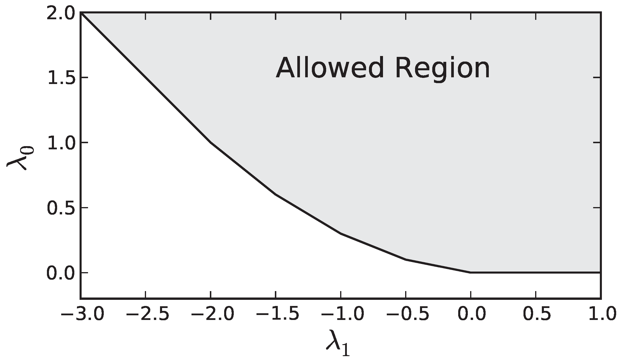
The set of constraints defines a convex region in the
,
plane as seen in
Figure A1. The minimum of our dual objective generically occurs at a vertex of the boundary of the allowed region, or possibly degenerate minima can occur anywhere along an edge of the region. From
Figure A1 is is clear that this occurs where Equation (
A12) is an equality for two (or three in the degenerate case) consecutive values of
i. Calling the first of these two values
, we then have the following two equations that allow us to determine the optimal values of
and
(
and
, respectively) as a function of
Figure A1.
An example of the allowed values of and for the dual problem ().
Figure A1.
An example of the allowed values of and for the dual problem ().
Solving for
and
, we find
Plugging this into Equation (
A11) we find the optimal value
is
Now all that is left is to express
as a function of
and take the limit as
N becomes large. This expression can be found by noting from Equation (
A11) and
Figure A1 that at the solution,
satisfies
where
is the slope,
, of constraint
i. The expression for
is determined from Equation (
A12),
Substituting Equation (
A19) into Equation (
A18), we find
This allows us to write
where
is between 0 and 1 for all
N. Solving this for
, we obtain
Substituting Equation (
A22) into Equation (
A17), we find
Taking the large
N limit we find that
and by the principle of strong duality [
52] the maximum value of
is
. Therefore we have shown that for large
N, the region of satisfiable constraints is simply
as illustrated in
Figure A2.
Figure A2.
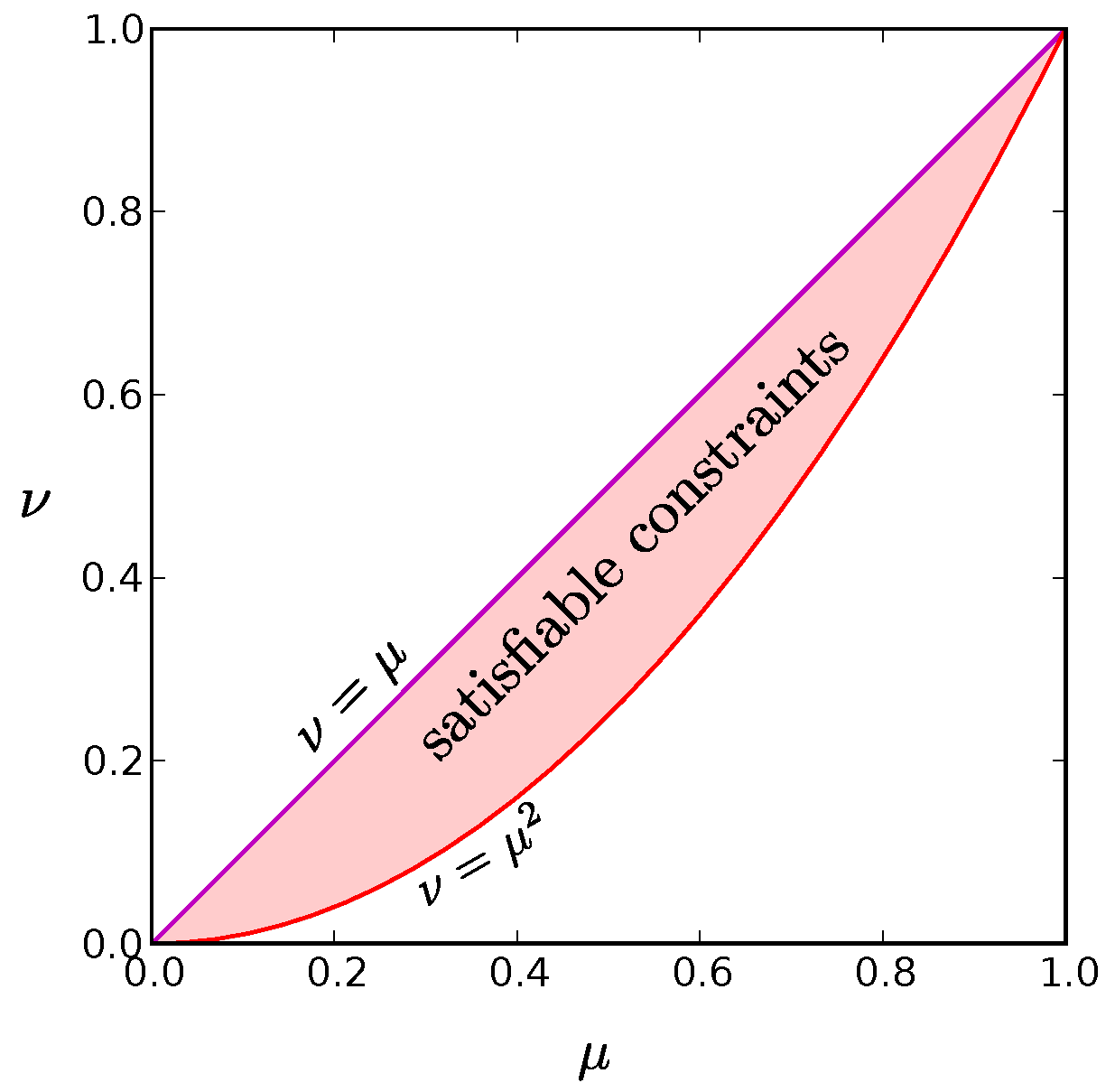
The red shaded region is the set of values for and that can be satisfied for at least one probability distribution in the limit. The purple line along the diagonal where is the distribution for which only the all active and all inactive states have non-zero probability. It represents the global entropy minimum for a given value of . The red parabola, , at the bottom border of the allowed region corresponds to a wide range of probability distributions, including the global maximum entropy solution for given in which each neuron fires independently. We find that low entropy solutions reside at this low boundary as well.
Figure A2.
The red shaded region is the set of values for and that can be satisfied for at least one probability distribution in the limit. The purple line along the diagonal where is the distribution for which only the all active and all inactive states have non-zero probability. It represents the global entropy minimum for a given value of . The red parabola, , at the bottom border of the allowed region corresponds to a wide range of probability distributions, including the global maximum entropy solution for given in which each neuron fires independently. We find that low entropy solutions reside at this low boundary as well.
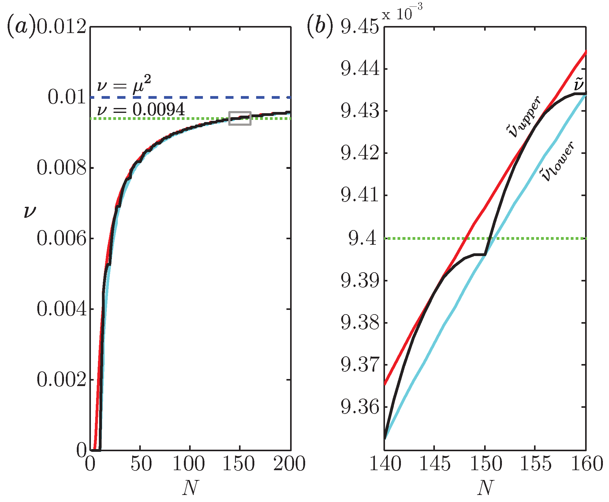
We can also compute upper and lower bounds on the minimum possible value for
for finite
N by taking the derivative of
(Equation (
A23)) with respect to
and setting that to zero, to obtain
. Recalling that
, it is clear that the only candidates for extremizing
are
, and we have:
To obtain the exact value of the minimum of
for finite
N, we substitute the greatest integer less than or equal to
for
in Equation (
A17) to obtain
where
is the floor function. Both of the bounds in (
A25) and the true
are plotted as functions of
N in
Figure 3 of the main text for
.
Appendix B. Minimum Entropy Occurs at Small Support
Our goal is to minimize the entropy function
where
is the number of states, the
satisfy a set of
independent linear constraints, and
for all
i. For the main problem we consider,
. The constraints for normalization, mean firing rates, and pairwise firing rates give
In this section we will show that the minimum occurs at the vertices of the space of allowed probabilities. Moreover, these vertices correspond to probabilities of small support—specifically a support size equal to
in most cases. These two facts allow us to put an upper bound on the minimum entropy of
for large
N.
We begin by noting that the space of normalized probability distributions
is the standard simplex in
dimensions. Each linear constraint on the probabilities introduces a hyperplane in this space. If the constraints are consistent and independent, the intersection of these hyperplanes defines a
affine space, which we call
. All solutions are constrained to the intersection between
and
and this solution space is a convex polytope of dimension ≤
d, which we refer to as
. A point within a convex polytope can always be expressed as a linear combination of its vertices, therefore if
are the vertices of
we may write
where
is the total number of vertices and
.
Using the concavity of the entropy function, we will now show that the minimum entropy for a space of probabilities
S is attained on the vertices of that space. Of course, this means that the global minimum will occur at the vertex that has the lowest entropy,
Moreover, if a distribution satisfying the constraints exists, then there is one with at most
non-zero
(e.g., from arguments as in [
41]). Together, these two facts imply that there are minimum entropy distributions with a maximum of
non-zero
. This means that even though the state space may grow exponentially with
N, the support of the minimum entropy solution for fixed means and pairwise correlations will only scale quadratically with
N.
This allows us to give an upper bound on the minimum entropy as,
for large
N. It is important to note how general this bound is: as long as the constraints are independant and consistent this result holds
regardless of the specific values of the
and
.
Appendix C. The Maximum Entropy Solution
In the previous Appendix, we derived a useful upper bound on the minimum entropy solution valid for any values of
and
that can be achieved by at least one probability distribution. In
Appendix H below, we obtain a useful lower bound on the minimum entropy solution. It is straightforward to obtain an upper bound on the maximum entropy distribution valid for arbitrary achievable
and
: the greatest possible entropy for
N neurons is achieved if they all fire independently with probability
, resulting in the bound
.
Deriving a useful lower bound for the maximum entropy for arbitrary allowed constraints and is a subtle problem. In fact, merely specifying how an ensemble of binary units should be grown from some finite initial size to arbitrarily large N in such a way as to “maintain” the low-level statistics of the original system raises many questions.
For example, typical neural populations consist of units with varying mean activities, so how should the mean activities of newly added neurons be chosen? For that matter, what correlational structure should be imposed among these added neurons and between each new neuron and the existing units? For each added neuron, any choice will inevitably change the histograms of mean activities and pairwise correlations for any initial ensemble consisting of more than one neuron, except in the special case of uniform constraints. Even for the relatively simple case of uniform constraints, we have seen that there are small systems that cannot be grown beyond some critical size while maintaining uniform values for
and
(see
Figure 2 in the main text). The problem of determining whether it is even mathematically possible to add a neuron with some predetermined set of pairwise correlations with existing neurons can be much more challenging for the general case of nonuniform constraints.
For these reasons, we will leave the general problem of finding a lower bound on the maximum entropy for future work and focus here on the special case of uniform constraints:
We will obtain a lower bound on the maximum entropy of the system with the use of an explicit construction, which will necessarily have an entropy,
, that does not exceed that of the maximum entropy solution. We construct our model system as follows: with probability
, all
N neurons are active and set to 1, otherwise each neuron is independently set to 1 with probability
. The conditions required for this model to match the desired mean activities and pairwise correlations across the population are given by
Inverting these equations to isolate
and
yields
The entropy of the system is then
where
w and
x are nonnegative constants for all allowed values of
and
that can be achieved for arbitrarily large systems.
x is nonzero provided
( i.e.,
), so the entropy of the system will grow linearly with
N for any uniform constraints achievable for arbitrarily large systems except for the case in which all neurons are perfectly correlated.
Using numerical methods, we can empirically confirm the linear scaling of the entropy of the true maximum entropy solution for the case of uniform constraints that can be achieved by arbitrarily large systems. In general, the constraints can be written
where the sums run over all
states of the system. In order to enforce the constraints, we can add terms involving Lagrange multipliers
and
to the entropy in the usual fashion to arrive at a function to be maximized
Maximizing this function gives us the Boltzmann distribution for an Ising spin glass
where
is the normalization factor or partition function. The values of
and
are left to be determined by ensuring this distribution is consistent with our constraints
and
.
For the case of uniform constraints, the Lagrange multipliers are themselves uniform:
This allows us to write the following expression for the maximum entropy distribution:
If there are
k neurons active, this becomes
Note that there are
states with probability
. Using expression (
A48), we find the maximum entropy by using the
fsolve function from the
SciPy package of Python subject to constraints (
A34) and (
A35).
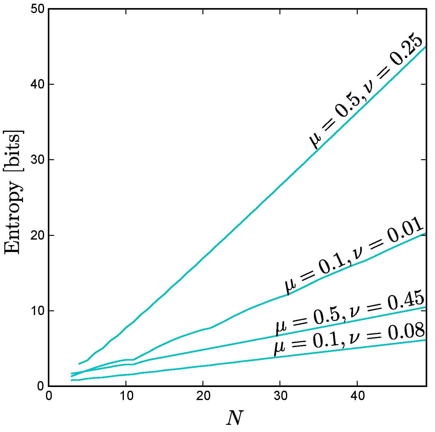
As
Figure A3 shows, for fixed uniform constraints the entropy scales linearly as a function of
N, even in cases where the correlations between all pairs of neurons (
) are quite large, provided that
. Moreover, for uniform constraints with anticorrelated units ( i.e., pairwise correlations
below the level one would observe for independent units), we find empirically that the maximum entropy still scales approximately linearly up to the maximum possible system size consistent with these constraints, as illustrated by
Figure 3 in the main text.
Figure A3.
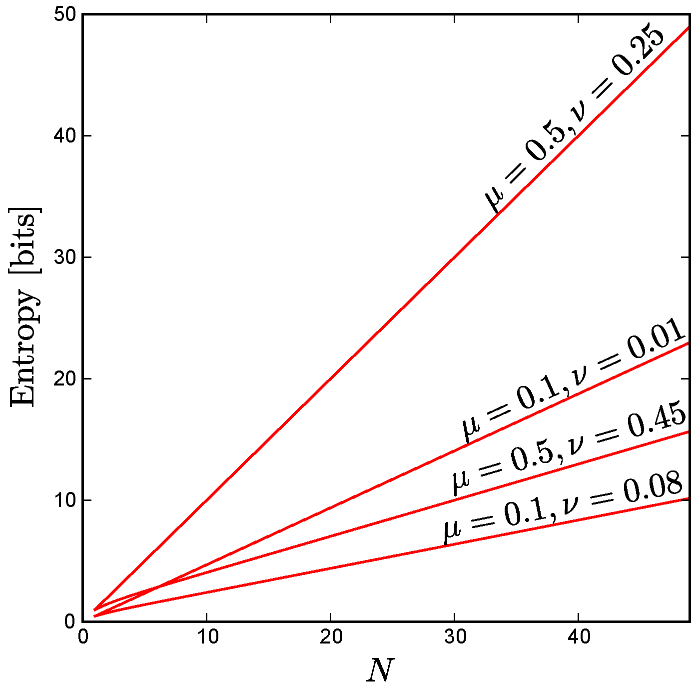
For the case of uniform constraints achievable by arbitrarily large systems, the maximum possible entropy scales linearly with system size, N, as shown here for various values of and . Note that this linear scaling holds even for large correlations, provided that . For the extreme case , all the neurons are perfectly correlated so the entropy of the ensemble does not change with increasing N.
Figure A3.
For the case of uniform constraints achievable by arbitrarily large systems, the maximum possible entropy scales linearly with system size, N, as shown here for various values of and . Note that this linear scaling holds even for large correlations, provided that . For the extreme case , all the neurons are perfectly correlated so the entropy of the ensemble does not change with increasing N.
Appendix D. Minimum Entropy for Exchangeable Probability Distributions
Although the values of the firing rate () and pairwise correlations () may be identical for each neuron and pair of neurons, the probability distribution that gives rise to these statistics need not be exchangeable as we have already shown. Indeed, as we explain below, it is possible to construct non-exchangeable probability distributions that have dramatically lower entropy then both the maximum and the minimum entropy for exchangeable distributions. That said, exchangeable solutions are interesting in their own right because they have large N scaling behavior that is distinct from the global entropy minimum, and they provide a symmetry that can be used to lower bound the information transmission rate close to the maximum possible across all distributions.
Restricting ourselves to exchangeable solutions represents a significant simplification. In the general case, there are
probabilities to consider for a system of
N neurons. There are
N constraints on the firing rates (one for each neuron) and
pairwise constraints (one for each pair of neurons). This gives us a total number of constrains (
) that grows quadratically with
N:
However in the exchangeable case, all states with the same number of spikes have the same probability so there are only
free parameters. Moreover, the number of constraints becomes 3 as there is only one constraint each for normalization, firing rate, and pairwise firing rate (as expressed in Equations (
A5)–(
A7), respectively). In general, the minimum entropy solution for exchangeable distributions should have the minimum support consistent with these three constraints. Therefore, the minimum entropy solution should have at most three non-zero probabilities (see
Appendix B).
For the highly symmetrical case with
and
, we can construct the exchangeable distribution with minimum entropy for all even
N. This distribution consists of the all ones state, the all zeros state, and all states with
ones. The constraint
implies that
, and the condition
implies
which corresponds to an entropy of
Using Sterling’s approximation and taking the large
N limit, this simplifies to
For arbitrary values of , and N, it is difficult to determine from first principles which three probabilities are non-zero for the minimum entropy solution, but fortunately the number of possibilities is now small enough that we can exhaustively search by computer to find the set of non-zero probabilities corresponding to the lowest entropy.
Using this technique, we find that the scaling behavior of the exchangeable minimum entropy is linear with
N as shown in
Figure A4. We find that the asymptotic slope is positive, but less than that of the maximum entropy curve, for all
. For the symmetrical case,
, our exact expression Equation (
A51) for the exchangeable distribution consisting of the all ones state, the all zeros state, and all states with
ones agrees with the minimum entropy exchangeable solution found by exhaustive search, and in this special case the asymptotic slope is identical to that of the maximum entropy curve.
Figure A4.
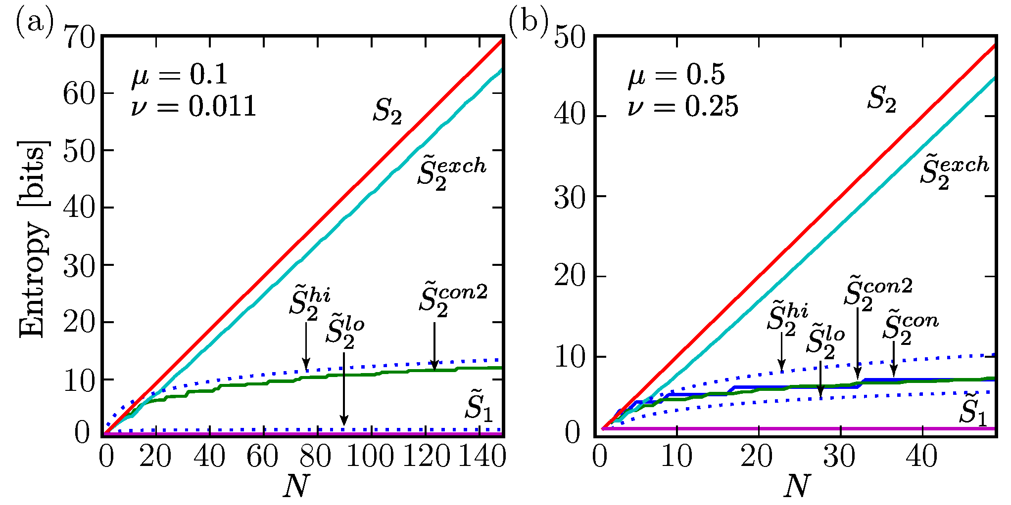
The minimum entropy for exchangeable distributions versus N for various values of and . Note that, like the maximum entropy, the exchangeable minimum entropy scales linearly with N as , albeit with a smaller slope for . We can calculate the entropy exactly for = 0.5 and = 0.25 as , and we find that the leading term is indeed linear: .
Figure A4.
The minimum entropy for exchangeable distributions versus N for various values of and . Note that, like the maximum entropy, the exchangeable minimum entropy scales linearly with N as , albeit with a smaller slope for . We can calculate the entropy exactly for = 0.5 and = 0.25 as , and we find that the leading term is indeed linear: .
Appendix E. Construction of a Low Entropy Distribution for All Values of μ and ν
We can construct a probability distribution with roughly
states with nonzero probability out of the full
possible states of the system such that
where
N is the number of neurons in the network and
n is the number of neurons that are active in every state. Using this solution as a basis, we can include the states with all neurons active and all neurons inactive to create a low entropy solution for all allowed values for
and
(See
Appendix G). We refer to the entropy of this low entropy construction
to distinguish it from the entropy (
) of another low entropy solution described in the next section. Our construction essentially goes back to Joffe [
60] as explained by Luby in [
33].
We derive our construction by first assuming that N is a prime number, but this is not actually a limitation as we will be able to extend the result to all values of N. Specifically, non-prime system sizes are handled by taking a solution for a larger prime number and removing the appropriate number of neurons. It should be noted that occasionally the solution derived using the next largest prime number does not necessarily have the lowest entropy and occasionally we must use even larger primes to find the minimum entropy possible using this technique; all plots in the main text were obtained by searching for the lowest entropy solution using the 10 smallest primes that are each at least as great as the system size N.
We begin by illustrating our algorithm with a concrete example; following this illustrative case we will prove that each step does what we expect in general. Consider , and . The algorithm is as follows:
Begin with the state with active neurons in a row:
Generate new states by inserting progressively larger gaps of 0s before each 1 and wrapping active states that go beyond the last neuron back to the beginning. This yields unique states including the original state:
Finally, “rotate” each state by shifting each pattern of ones and zeros to the right (again wrapping states that go beyond the last neuron). This yields a total of states:
11100 01110 00111 10011 11001
10101 11010 01101 10110 01011
11010 01101 10110 01011 10101
10011 11001 11100 01110 00111
Note that each state is represented twice in this collection, removing duplicates we are left with
total states. By inspection we can verify that each neuron is active in
states and each pair of neurons is represented in
states. Weighting each state with equal probability gives us the values for
and
stated in Equation (
A53).
Now we will prove that this construction works in general for N prime and any value of n by establishing (1) that step 2 of the above algorithm produces a set of states with n spikes; (2) that this method produces a set of states that when weighted with equal probability yield neurons that all have the same firing rates and pairwise statistics; and (3) that this method produces at least double redundancy in the states generated as stated in step 4 (although in general there may be a greater redundancy). In discussing (1) and (2) we will neglect the issue of redundancy and consider the states produced through step 3 as distinct.
First we prove that step 2 always produces states with
n neurons, which is to say that no two spikes are mapped to the same location as we shift them around. We will refer to the identity of the spikes by their location in the original starting state; this is important as the operations in step 2 and 3 will change the relative ordering of the original spikes in their new states. With this in mind, the location of the
ith spike with a spacing of
s between them will result in the new location
l (here the original state with all spikes in a row is
):
where
. In this form, our statement of the problem reduces to demonstrating that for given values of
s and
N, no two values of
i will result in the same
l. This is easy to show by contradiction. If this were the case,
For this to be true, either s or must contain a factor of N, but each are smaller than N so we have a contradiction. This also demonstrates why N must be prime—if it were not, it would be possible to satisfy this equation in cases where s and contain between them all the factors of N.
It is worth noting that this also shows that there is a one-to-one mapping between
s and
l given
i. In other words, each spike is taken to every possible neuron in step 2. For example, if
, and we fix
:
If we now perform the operation in step 3, then the location
l of spike
i becomes
where
d is the amount by which the state has been rotated (the first column in step 3 is
, the second is
, etc.). It should be noted that step 3 trivially preserves the number of spikes in our states so we have established that steps 2 and 3 produce only states with
n spikes.
We now show that each neuron is active, and each pair of neurons is simultaneously active, in the same number of states. This way when each of these states is weighted with equal probability, we find symmetric statistics for these two quantities.
Beginning with the firing rate, we ask how many states contain a spike at location
l. In other words, how many combinations of
s,
i, and
d can we take such that Equation (
A56) is satisfied for a given
l. For each choice of
s and
i there is a unique value of
d that satisfies the equation.
s can take values between 1 and
, and
i takes values from 0 to
, which gives us
states that include a spike at location
l. Dividing by the total number of states
we obtain an average firing rate of
Consider neurons at
and
; we wish to know how many values of
s,
d,
and
we can pick so that
Taking the difference between these two equations, we find
From our discussion above, we know that this equation uniquely specifies
s for any choice of
and
. Furthermore, we must pick
d such that Equations (
A58) and (
A59) are satisfied. This means that for each choice of
and
there is a unique choice of
s and
d, which results in a state that includes active neurons at locations
and
. Swapping
and
will result in a different
s and
d. Therefore, we have
states that include any given pair—one for each choice of
and
. Dividing this number by the total number of states, we find a correlation
equal to
where
N is prime.
Finally we return to the question of redundancy among states generated by steps 1 through 3 of the algorithm. Although in general there may be a high level of redundancy for choices of n that are small or close to N, we can show that in general there is at least a twofold degeneracy. Although this does not impact our calculation of and above, it does alter the number of states, which will affect the entropy of system.
The source of the twofold symmetry can be seen immediately by noting that the third and fourth rows of our example contain the same set of states as the second and first respectively. The reason for this is that each state in the case involves spikes that are one leftward step away from each other just as involves spikes that are one rightward shift away from each other. The labels we have been using to refer to the spikes have reversed order but the set of states are identical. Similarly the case contains all states with spikes separated by two leftward shifts just as the case. Therefore, the set of states with is equivalent to the set of states with . Taking this degeneracy into account, there are at most unique states; each neuron spikes in of these states and any given pair spikes together in states.
Because these states each have equal probability the entropy of this system is bounded from above by
where
N is prime. As mentioned above, we write this as an inequality because further degeneracies among states beyond the factor of two that always occurs are possible for some prime numbers. In fact, in order to avoid non-monotonic behavior, the curves for
shown in
Figure 1 and
Figure 3 of the main text were generated using the lowest entropy found for the 10 smallest primes greater than
N for each value of
N.
We can extend this result to arbitrary values for
N including non-primes by invoking the Bertrand-Chebyshev theorem, which states that there always exists at least one prime number
p with
for any integer
:
where
N is any integer. Unlike the maximum entropy and the entropy of the exchangeable solution, which we have shown to both be extensive quantities, this scales only logarithmically with the system size
N.
Appendix F. Another Low Entropy Construction for the Communications Regime, &
In addition to the probability distribution described in the previous section, we also rediscovered another low entropy construction in the regime most relevant for engineered communications systems (
,
) that allows us to satisfy our constraints for a system of
N neurons with only
active states. Below we describe a recursive algorithm for determining the states for arbitrarily large systems—states needed for
are built from the states needed for
, where
q is any integer greater than 2. This is sometimes referred to as a Hadamard matrix. Interestingly, this specific example goes back to Sylvester in 1867 [
22], and it was recently discussed in the context of neural modeling by Macke and colleagues [
21].
We begin with
. Here we can easily write down a set of states that when weighted equally lead to the desired statistics. Listing these states as rows of zeros and ones, we see that they include all possible two-neuron states:
In order to find the states needed for
we replace each 1 in the above by
and each 0 by
to arrive at a new array for twice as many neurons and twice as many states with nonzero probability:
By inspection, we can verify that each new neuron is spiking in half of the above states and each pair is spiking in a quarter of the above states. This procedure preserves
,
, and
for all neurons; thus providing a distribution that mimics the statistics of independent binary variables up to third order (although it does not for higher orders). Let us consider the the proof that
is preserved by this transformation. In the process of doubling the number of states from
to
, each neuron with firing rate
“produces” two new neurons with firing rates
and
. It is clear from Equations (
A65) and (
A66) that we obtain the following two relations,
It is clear from these equations that if we begin with that this will be preserved by this transformation. By similar, but more tedious, methods one can show that , and .
Therefore, we are able to build up arbitrarily large groups of neurons that satisfy our statistics using only
states by repeating the procedure that took us from
to
. Since these states are weighted with equal probability we have an entropy that grows only logarithmically with
NWe mention briefly a geometrical interpretation of this probability distribution. The active states in this distribution can be thought of as a subset of corners on an N dimensional hypercube with the property that the separation of almost every pair is the same. Specifically, for each active state, all but one of the other active states has a Hamming distance of exactly from the original state; the remaining state is on the opposite side of the cube, and thus has a Hamming distance of N. In other words, for any pair of polar opposite active states, there are active states around the “equator”.
We can extend Equation (
A70) to arbitrary numbers of neurons that are not multiples of 2 by taking the least multiple of 2 at least as great as
N, so that in general:
By adding two other states we can extend this probability distribution so that it covers most of the allowed region for and while remaining a low entropy solution, as we now describe.
We remark that the authors of [
31,
34] provide a lower bound of
for the sample size possible for a pairwise independent binary distribution, making the sample size of our novel construction essentially optimal.
Appendix G. Extending the Range of Validity for the Constructions
We now show that each of these low entropy probability distributions can be generalized to cover much of the allowed region depicted in
Figure A2; in fact, the distribution derived in
Appendix E can be extended to include all possible combinations of the constraints
and
. This can be accomplished by including two additional states: the state where all neurons are silent and the state where all neurons are active. If we weight these states by probabilities
and
respectively and allow the
original states to carry probability
in total, normalization requires
We can express the value of the new constraints (
and
) in terms of the original constraint values (
and
) as follows:
These values span a triangular region in the
-
plane that covers the majority of satisfiable constraints.
Figure A5 illustrates the situation for
. Note that by starting with other values of
, we can construct a low entropy solution for any possible constraints
and
.
With the addition of these two states, the entropy of the expanded system
is bounded from above by
For given values of
and
, the
are fixed and only the first term depends on
N. Using Equations (
A73) and (
A74),
This allows us to rewrite Equation (
A75) as
We are free to select
and
to minimize the first coefficient for a desired
and
, but in general we know this coefficient is less than 1 giving us a simple bound,
Like the original distribution, the entropy of this distribution scales logarithmically with
N. Therefore, by picking our original distribution properly, we can find low entropy distributions for any
and
for which the number of active states grows as a polynomial in
N (see
Figure A5).
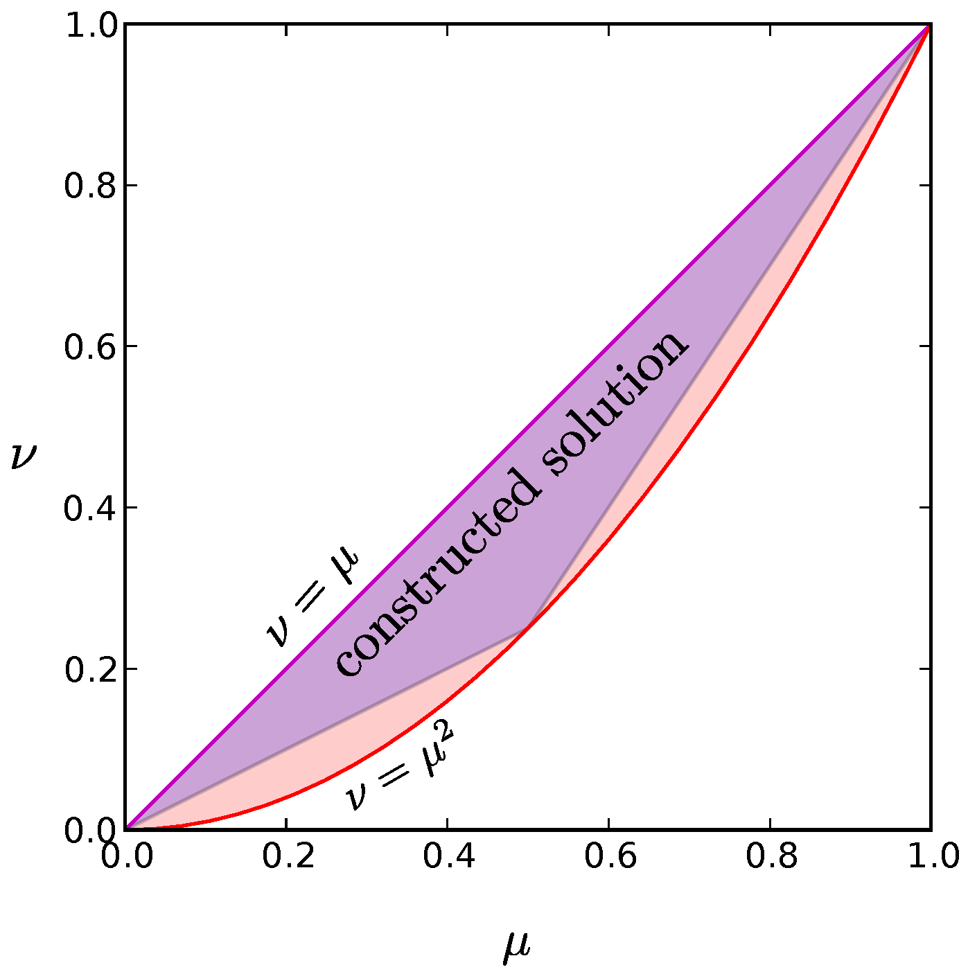
Figure A5.
The full shaded region includes all allowed values for the constraints
and
for all possible probability distributions, replotted from
Figure A2. As described in
Appendix E and
Appendix G, one of our low-entropy constructed solutions can be matched to any of the allowed constraint values in the full shaded region, whereas the constructed solution described in
Appendix F can achieve any of the values within the triangular purple shaded region. Note that even with this second solution, we can cover most of the allowed region. Each of our constructed solutions have entropies that scale as
.
Similarly, we can extend the range of validity for the construction described in
Appendix F to the triangular region shown in
Figure A2 by assigning probabilities
,
, and
to the all silent state, all active state, and the total probability assigned to the remaining
states of the original model, respectively. The entropy of this extended distribution must be no greater than the entropy of the original distribution (Equation (
A71)), since the same number of states are active, but now they are not weighted equally, so this remains a low entropy distribution.
Appendix H. Proof of the Lower Bound on Entropy for Any Distribution Consistent with Given &
Using the concavity of the logarithm function, we can derive a lower bound on the minimum entropy. Our lower bound asymptotes to a constant except for the special case , ∀ i, and , ∀, which is especially relevant for communication systems since it matches the low order statistics of the global maximum entropy distribution for an unconstrained set of binary variables.
We begin by bounding the entropy from below as follows:
where
represents the full vector of all
state probabilities, and we have used
to denote an average over the distribution
. The third step follows from Jensen’s inequality applied to the convex function
.
Now we seek an upper bound on
. This can be obtained by starting with the matrix representation
C of the constraints (for now, we consider each state of the system,
, as a binary column vector, where
i denotes the state and each of the
N components is either 1 or 0):
where
C is an
matrix. In this form, the diagonal entries of
C,
, are equal to
and the off diagonal entries,
, are equal to
.
For the calculation that follows, it is expedient to represent words of the system as
rather than
( i.e., −1 represents a silent neuron instead of 0). The relationship between the two can be written
where
is the vector of all ones. Using this expression, we can relate
to
C:
Returning to Equation (
A80) to find an upper bound on
, we take the square of the Frobenius norm of
:
The final line is where our new representation pays off: in this representation,
. This gives us the desired upper bound for
:
Using Equations (
A84)–(
A86), we can express
in terms of
and
:
Combining this result with Equations (
A87) and (
A79), we obtain a lower bound for the entropy for any distribution consistent with any given sets of values
and
:
where
and
is the average value of
over all
with
.
In the case of uniform constraints, this becomes
where
.
For large values of
N this lower bound asymptotes to a constant
The one exception is when
. In the large
N limit, this case is limited to when
and
for all
i,
j. Each
is positive semi-definite; therefore,
only when each
. In other words,
But in the large
N limit,
Without loss of generality, we assume that
. In this case,
and
Of course, that means that in order to satisfy
each pair must have one
less than of equal to
and the other greater than or equal to
. The only way this may be true for all possible pairs is if all
are equal to
. According to Equation (
A96), all
must then be equal to
. This is precisely the communication regime, and in this case our lower-bound scales logarithmically with
N,

 ,
, 