Article

An Exploration Algorithm for Stochastic Simulators Driven by Energy Gradients

by
Anastasia S. Georgiou
1,
Juan M. Bello-Rivas
2,
Charles William Gear
1,
Hau-Tieng Wu
3,
Eliodoro Chiavazzo
4 and
Ioannis G. Kevrekidis
5,6,*
1
Department of Chemical and Biological Engineering, Princeton University, Princeton, NJ 08544, USA
2
Program in Applied and Computational Mathematics, Princeton University, Princeton, NJ 08544, USA
3
Department of Mathematics, University of Toronto, Room 6290, 40 St. George Street, Toronto, ON M5S 2E4, Canada
4
Energy Department, Politecnico di Torino, 10129 Torino, Italy
5
Department of Chemical and Biological Engineering and Program in Applied and Computational Mathematics, Princeton University, Princeton, NJ 08544, USA
6
TUM Institute for Advanced Study, Technische Universität München, 85748 Garching, Germany
*
Author to whom correspondence should be addressed.
Entropy 2017, 19(7), 294; https://doi.org/10.3390/e19070294
Submission received: 28 February 2017 / Revised: 24 April 2017 / Accepted: 8 May 2017 / Published: 22 June 2017
(This article belongs to the Special Issue Understanding Molecular Dynamics via Stochastic Processes)

Abstract

:
In recent work, we have illustrated the construction of an exploration geometry on free energy surfaces: the adaptive computer-assisted discovery of an approximate low-dimensional manifold on which the effective dynamics of the system evolves. Constructing such an exploration geometry involves geometry-biased sampling (through both appropriately-initialized unbiased molecular dynamics and through restraining potentials) and, machine learning techniques to organize the intrinsic geometry of the data resulting from the sampling (in particular, diffusion maps, possibly enhanced through the appropriate Mahalanobis-type metric). In this contribution, we detail a method for exploring the conformational space of a stochastic gradient system whose effective free energy surface depends on a smaller number of degrees of freedom than the dimension of the phase space. Our approach comprises two steps. First, we study the local geometry of the free energy landscape using diffusion maps on samples computed through stochastic dynamics. This allows us to automatically identify the relevant coarse variables. Next, we use the information garnered in the previous step to construct a new set of initial conditions for subsequent trajectories. These initial conditions are computed so as to explore the accessible conformational space more efficiently than by continuing the previous, unbiased simulations. We showcase this method on a representative test system.

1. Introduction

In its most straightforward formulation, Molecular Dynamics (MD) consists of solving Newton’s equations of motion for a molecular system described with atomic resolution. The goal of performing MD simulations is twofold: on the one hand, we want to gather samples from a given thermodynamic ensemble, while, on the other hand, we may seek to gain insight into time-dependent behavior. The first objective leads us to equilibrium properties. The second yields kinetic properties and is the reason why it is said that MD acts as a computational microscope. Recent success stories involving systems having more than one million atoms [1,2] attest to the ever-growing reach of MD simulations.
The possibility of using MD to study bigger bio-molecules at longer time scales is hindered by the problem of time scale separation. While the processes of interest (protein folding, permeation of cellular membranes, etc.) act on timescales of milliseconds to minutes, we are currently restricted by limitations in available computer capabilities and algorithms to simulations spanning timescales of microseconds. Moreover, to ensure stability when numerically integrating the equations of motion, we need to take steps of just a few femtoseconds. The reader interested in the numerical analysis of integration schemes in MD is referred to the excellent treatise [3] for more information.
The inherent difficulty behind the problem of timescale separation lies in the fact that many biophysical systems display metastability. That is, the solutions of the equations of motion spend large amounts of time trapped in the basins of attraction of local free energy minima, called metastable states [4,5]. While visiting these regions of the conformational space, nothing remarkable happens until the system reaches a new metastable state and, eventually, a global free energy minimum. Many computer simulation techniques have been proposed to address this problem by accelerating the sampling of the conformational space and enhancing the statistics of the transitions between metastable states. An incomplete list of these schemes includes: accelerated molecular dynamics [6], adaptive biasing force [7,8], forward flux sampling [9], locally-enhanced sampling [10], Markov state models [11,12,13,14,15], metadynamics [16,17], milestoning [18,19], nudged elastic band [20,21,22], replica exchange molecular dynamics [23], simulated tempering [24,25], steered molecular dynamics [26], the string method [27,28], transition path sampling [29,30], transition interface sampling [31], umbrella sampling [32,33], weighted ensemble [34,35], etc. We refer the reader to recent surveys [36,37,38] for more complete and up-to-date overviews.
It is often possible to identify a suitable set of so-called collective or coarse variables describing the progress of the process being studied (i.e., a “slow manifold”). The simplest such “coarse variable” is perhaps the interatomic distance in the process of the dissociation of a diatomic molecule. In other cases, a subset of dihedral angles on the amino acids of a peptide proves to be a good choice. In practice, it is not always clear how to devise good coarse variables a priori, and it is necessary to rely on the expertise of computational chemists to postulate these variables with varying degrees of success. Of course, the quality of the coarse variables can be assessed a posteriori by methods such as the histogram test, etc. [30,39,40,41,42,43]. Ideally, the dynamics of the process mapped onto the coarse variables should be a diffusion on the potential of mean force (i.e., Smoluchowski equation) [44,45], but if the guessed variables are not good enough, they will be poor representations of the process of interest in that the relevant dynamics will be described instead by Generalized Langevin Equations (GLE) [46,47]. The GLE incorporates a history-dependent term that complicates computations [48].
In this paper, we present a detailed account of the iMapD [49] method. This can be used as a basin-hopping [50] simulation technique that lends itself naturally to parallelization, and unlike most of the methods referenced above, it does not require a priori guesses on the nature of the coarse variables. The method works by (a) performing short simulations to obtain an ensemble of trajectories; (b) using data mining techniques (diffusion maps) to automatically obtain an optimal set of local coarse variables that describe the conformations sampled by these trajectories and (c) using that knowledge to generate a new set of conformations. The new conformations become initial conditions for a new batch of short simulations, which, by construction, are more likely to lead to the exploration of new, previously unexplored local free energy minima. Throughout these steps, the algorithm constructs a representation of the intrinsic geometry of the visited region of the conformational space and identifies the points from which a new trajectory may have more chances to exit the metastable basins already visited. It is worth stressing that, as opposed to our previous work [49], here, we use a non-linear scheme to lift into the ambient space the extended boundary points. Moreover (and importantly), preliminary results are also reported on an alternative manifold parameterization based on what we will call sine-diffusion maps.
The paper is organized as follows. Section 2 provides a brief introduction to Diffusion Maps (DMAPS) from the perspective of statistical mechanics, followed by an overview of the iMapD method, as well as an application of the algorithm to a model problem. Section 3 is an account of the required mathematical tools upon which the iMapD method is built; namely, we discuss some technical aspects of diffusion maps, boundary detection methods, out-of-sample extension using geometric harmonics, and the use of local principal component analysis as an alternative to diffusion maps. Finally, Section 3.6 contains a more in-depth treatment of the steps involved in the iMapD algorithm, describing how the previously introduced building blocks fit within the method and exploring factors affecting the implementation of the method.

2. Diffusion Maps and the iMapD Algorithm

2.1. Diffusion Maps in Statistical Mechanics

Consider a mechanical system whose conformational space is denoted by Ω . For the sake of simplicity, let us assume that Ω R n is a bounded, simply-connected open set and that the system undergoes Brownian dynamics; that is, its time evolution is a solution of the Stochastic Differential Equation (SDE):
d x = U ( x )   d t + 2 β 1   d W ,
where U = U ( x ) is the potential energy, β 1 > 0 is the inverse temperature and W is a standard n-dimensional Brownian motion [51,52]. Potential energy functions in MD simulations are not smooth in general, but equilibrium trajectories almost never visit the singular points, so it is safe to assume that U is sufficiently smooth.
Let:
P ( A , t | x ) = A p ( y , t | x )   d y
be the probability that a trajectory of (1) started at x Ω at time t = 0 belongs to the set A Ω at time t 0 . It is known that the time evolution of the probability density function p is governed by the Fokker–Planck equation [53],
p t = · ( β 1 p + p U ) , in   Ω × ( 0 , ) , n ( β 1 p + p U ) = 0 , on   Ω × ( 0 , ) , p ( · , 0 | x ) = δ x , on   Ω × { 0 } ,
where n denotes the derivative in the direction of the unit normal vector to the boundary Ω of the conformational space Ω and δ x is a Dirac delta function centered at x. In the context of molecular simulation, there are other boundary conditions that are relevant such as periodic boundary conditions or prescribed decay at infinity (i.e., lim x + p ( x , t ) = 0 for all t 0 , useful when Ω is unbounded).
We will refer to the operator on the right-hand side of the partial differential equation in (3) by the symbol L . That is, L p = · β 1 p + p U . By the spectral properties of the operator L and its adjoint L , we know [15,54] that p admits a decomposition of the form:
p ( y , t | x ) = i = 0 e λ i t ψ i ( y )   e β U ( y ) ψ i ( x ) ,
where λ 0 = 0 > λ 1 λ 2 are the eigenvalues of L , the sequence of eigenvalues satisfies lim n λ n = and ψ i ( x ) are the corresponding eigenfunctions. Observe that ψ 0 ( x ) = 1 for all x Ω . In Figure 1, we show the eigenfunctions of the operator L for a simple double well potential.
For systems with time scale separation, there will arise a spectral gap; that is, λ k + 1 λ k for some k N . Under such circumstances, (4) can be approximated as:
p ( y , t | x ) e β U ( y ) + i = 1 k e λ i t ψ i ( y )   e β U ( y ) ψ i ( x ) ,
and for a fixed value of ε λ k , we can construct the mapping:
x Ψ ε ( x ) = e λ 1 ε ψ 1 ( x ) , , e λ k ε ψ k ( x ) .
The components of Ψ ε are then, in effect, coarse variables that describe the state of the system. Therefore, the dimensionality reduction in diffusion maps stems from the existence of a spectral gap, and the effective dimension will be equal to k. These coarse variables are well suited to parameterize and study the free energy of the system.
Observe that the parameter ε > 0 plays the role of time in (4) and that events occurring at a rate smaller than ε 1 are ignored. This interpretation of ε suggests that one could use a priori knowledge of the dynamics of the system (e.g., frequency of bond vibrations, etc.) to set its value. Frequently, however, no such information is available. An optimal choice of ε was introduced in [56]. The optimal ε depends on the dimension of the space of coarse variables and the geometry of the manifold, as well as on the number of samples available.
The explicit computation of the eigenfunctions ψ i is infeasible in practical applications, so our focus naturally shifts to the numerical estimation of these eigenfunctions up to a prescribed accuracy. Diffusion Maps (DMAPS) are a manifold learning technique that allows us to obtain these approximations to ψ i by studying sets of points sampled from the solution of (1) at different instants (e.g., we take y 1 = x ( t 1 ) , , y m = x ( t m ) for some t 1 , , t m 0 ). The procedure is as follows: we first construct the m × m matrix:
W i j = exp y i y j 2 2 ε ,
where · is a suitable norm in R m (the Euclidean norm or a “Mahalanobis-like” distance [57,58] are typical choices). The next step for the construction of the diffusion map is the definition of the matrix W ˜ with entries:
W ˜ i j = W i j q i 1 / 2   q j 1 / 2 , where q i = j W i j .
By multiplying W ˜ by the inverse of the diagonal matrix D, with entries D i i = j W ˜ i j , we obtain a non-negative row-stochastic matrix, K = D 1 W ˜ . The matrix K gives us the transition probability of a Markov chain defined on the discrete state space { y 1 , , y m } determined by the observed data.
The matrix L = K I , where I is the m × m identity matrix, is known as the random walk Laplacian [59]. It can be proven [60] that the eigenvectors of the random walk Laplacian L converge to the eigenfunctions of the operator L . Thus, the numerical solution of the eigenproblem L ψ = λ ψ yields an effective, data-driven approximation method to compute (5). For example, in the case of the double well potential that we considered before, we obtain the eigenvectors displayed in Figure 2.
As a more realistic example, we analyze a one microsecond-long simulation of the catalytic domain of the human tyrosine protein kinase ABL1 [62]. This is a published dataset [63] that was generated on Folding@home [64] using OpenMM [65] 6.3.1 with the AMBER99SB-ILDNforce field [66], the TIP3Pwater model [67] and Cl and Na ions to neutralize the charge. To solve the Langevin dynamics equation, the stochastic position Verlet integrator [68,69] was used with a time step length of 2 fs at a temperature of 300 K with a collision rate (also known as the friction term) equal to 1 ps 1 . To treat electrostatic interactions, the smooth particle-mesh Ewald method [70] was used with a cut off of 1 nm and a tolerance of 5 × 10 4 . Pressure control was exerted by a molecular-scaling Monte Carlo barostat [71,72] using a 1-atm reference pressure attempting Monte Carlo moves every 50 steps.
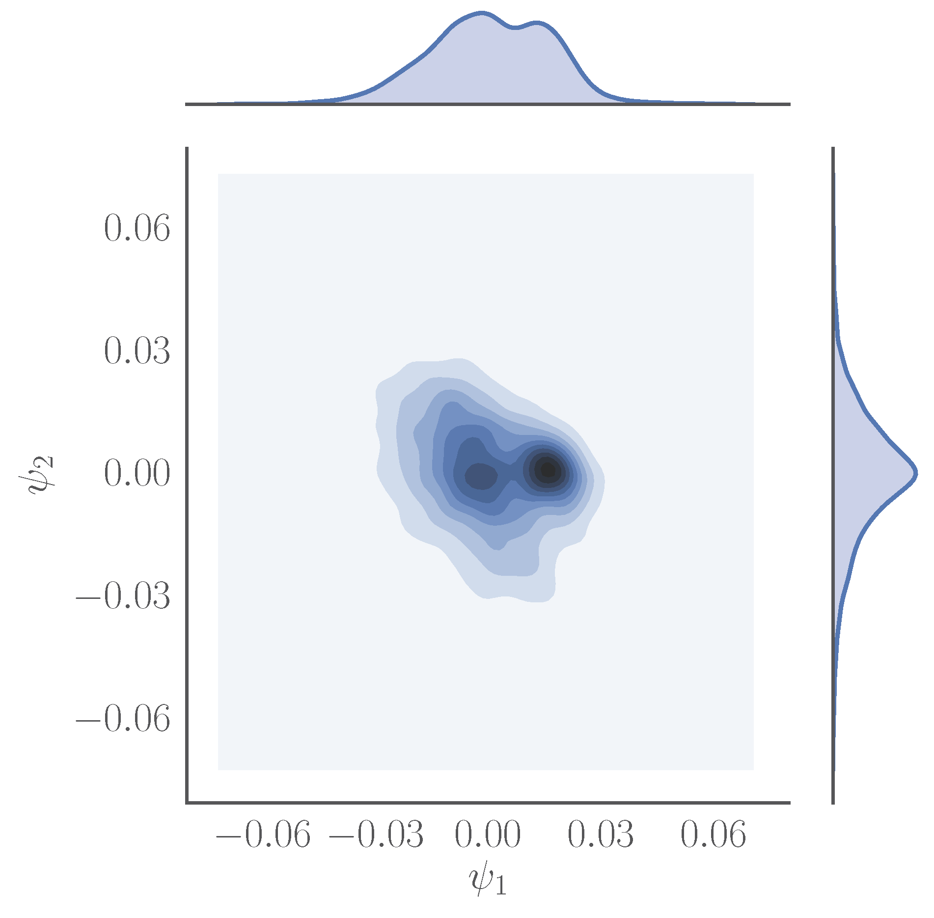
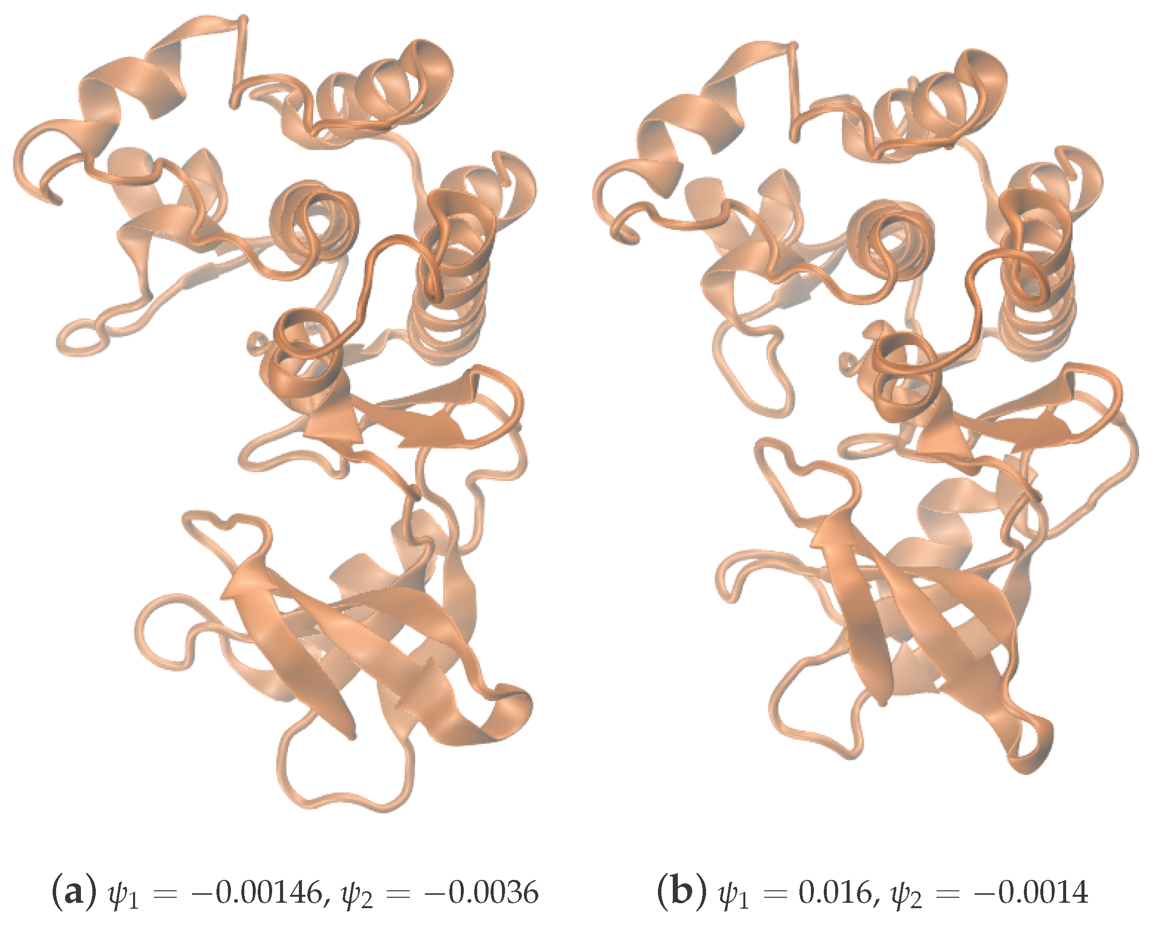
We obtain the first two coarse variables, ψ 1 and ψ 2 , using the diffusion map method (see Figure 3 and Figure 4 for the results).
The previous considerations are motivated by/conform with statistical mechanics; however, it is important to emphasize that the DMAPS method will work, in the sense that it will provide a parameterization of the manifold, just as well with data points on the manifold not necessarily coming from sampling the solution of (3). What is important is the geometry of the manifold and not necessarily the dynamics of the process leading to the samples. Indeed, we have used the framework of statistical mechanics for didactic purposes, but practical applications need not rely on it.

2.2. Overview of the iMapD Method

As we stated in the Introduction, the iMapD method is aimed at enhancing the sampling of unexplored regions of the conformational space of a system. The method works by first running an ensemble of independent trajectories initialized from an initial configuration for a short time (e.g., a few nanoseconds). The points comprising the trajectories are actually samples of the local free energy minimum to which the initial configuration belongs. Next, we perform a diffusion map computation, giving us a set of coarse variables that parameterize the current basin of attraction, and we locate (in DMAP coordinates) the boundary of the region that our set of points has explored so far. By extending the boundary outwards in its normal direction, we get a new tentative boundary whose points we realize in the original, high-dimensional conformational space (typically by resorting to a suitable biasing potential). Finally, the new points are used as initial conditions in a new batch of simulations. By actively restarting simulations from the extrapolated points, we enhance the ability of the system to exit local free energy minima and to explore new regions of conformational space.
In order to illustrate the applicability of our method, we demonstrate how the algorithm works on a simple, yet non-trivial model system, which can be studied in-depth by numerically solving the stochastic differential equations involved.
Let:
θ ( x , z ) = π / 2 arctan ( z / x ) , if   x < 0 , z < 0 , π / 2 + arctan ( z / x ) , if   x > 0 , z < 0 , arctan ( x / z ) , otherwise ,
and let:
γ ( x , y , z ) = 4   c R   θ ( x , z )   R   θ ( x , z ) 1 R   θ ( x , z ) + 1 b y ,
where b = 80 , c = 20 and R = 4 / π . Consider the system of stochastic differential equations (SDEs):
d x = η 1 x R   sin θ + γ cos θ d t + D 2   d W 1 , d y = ( 2 a y b   R   θ )   d t + D 2   d W 2 , d z = η 1 z R   cos θ γ sin θ d t + D 2   d W 3 ,
where a = 200 , D = 0.35 , η = 1 × 10 4 and W 1 , W 2 , W 3 are independent standard Brownian motions.
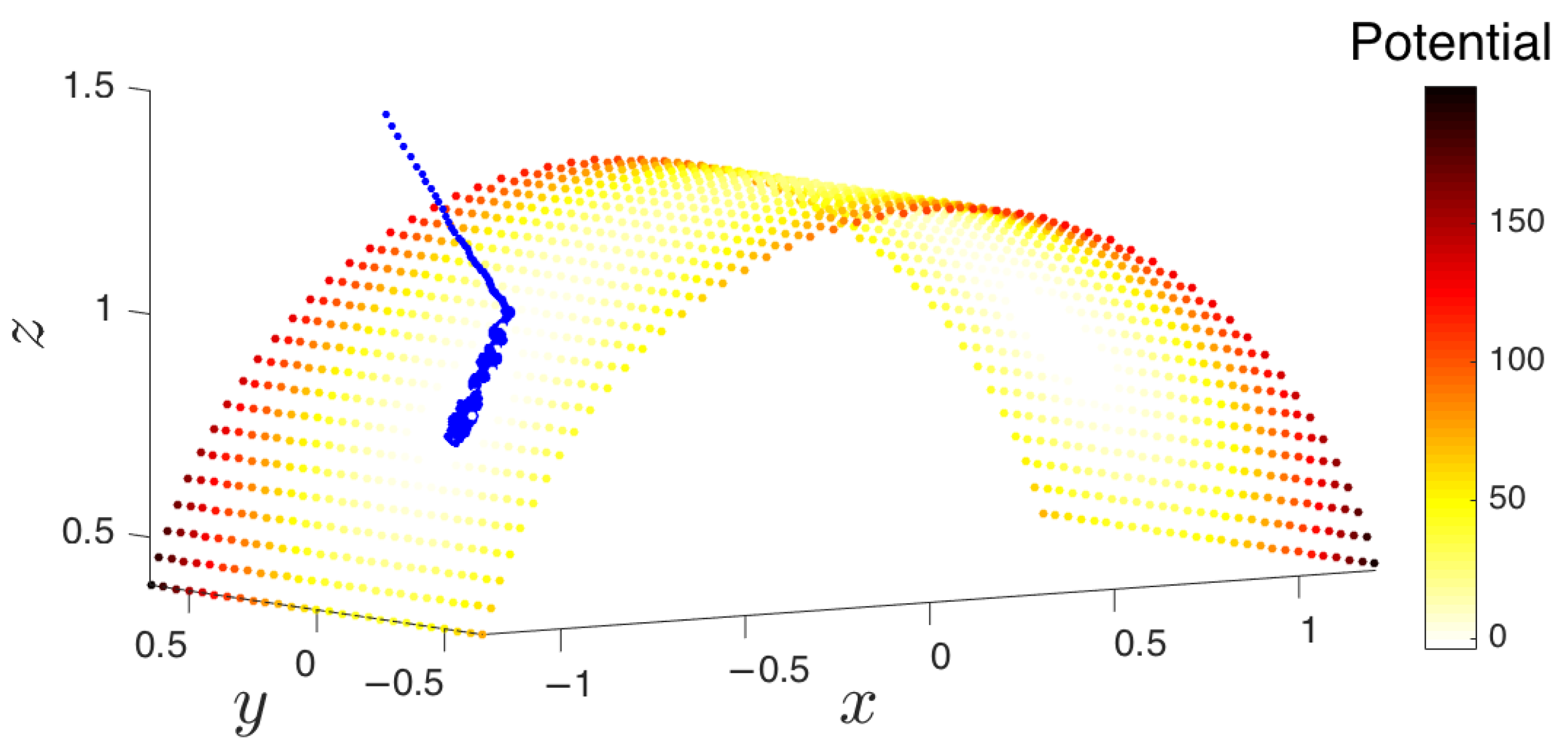
The above system of SDEs exhibits the most meaningful qualitative aspect of the type of problems that iMapD is designed for: a phase space with higher dimensionality than that of the manifold in which the effective dynamics occurs. Indeed, our system, despite being three-dimensional, has by construction a two-dimensional attractor located on the surface of a cylinder with radius R and axis y. There are two metastable states (as seen in Figure 5), and trajectories starting away from the attractor arrive at one of the metastable wells, where they remain for typically long periods of time.
In order to sample the conformational space of the system, we begin by running a single trajectory for enough time such that it gets trapped into one of the metastable sets. We process the trajectory so that the initial transient descent is removed, and points on the manifold have a more uniform distribution (e.g., by removing nearest neighbors that are closer than a fixed minimum distance). We then locate the boundary of the currently sampled area by running the alpha-shapes boundary detection method, which will be described in Section 3.3. This method is appropriate here, given that the manifold is two-dimensional and there is a correspondence between the points lying at the edge in the conformational space and the points at the edge in diffusion map space. Next, the boundary points in diffusion map space are extended using extrapolation and subsequently lifted up to the conformational space using geometric harmonics, which will be discussed in Section 3.5. Finally, the system is reinitialized, and the process starts over again, increasing the volume (here, the area) of explored conformational space and getting closer to the other metastable state. Figure 6 illustrates the first few steps in this process in conformational space and DMAP space, and Figure 7 shows how the extrapolated points approach the other basin as the algorithm marches on.
To create Figure 6 and Figure 7, the first trajectory was started with an arbitrary initial condition of ( 1.06 , 0.05 , 1.50 ) and run until t = 0.15 using the Euler–Maruyama scheme [73] with a time step length of 3 × 10 7 . In each iteration of the algorithm, and therefore each run of the molecular simulator, the first 600 samples were discarded to increase the likelihood that the resulting cloud of points rested on the cylindrical manifold. To make the manifold sampling more homogeneous, points were removed such that a minimum distance of 0.04 existed between each pair of points. A maximum of 3000 points was stored in memory at any given time; this parameter was based on the available memory of the machine at hand and the particular implementation of the method. Points were randomly pruned if this maximum threshold was surpassed. Once the point cloud was properly conditioned, the manifold boundary was extended by a distance of 0.25 spatial units.
To further illustrate the expansion of the point-cloud throughout the iterative process, we show in Table 1 the difference between the maximum and minimum angles of the set of points. This indicates how the iterative method explores the metastable sets on the cylinder.

3. Algorithmic Building Blocks

In this section we introduce several techniques on which the iMapD method relies. Section 3.1 continues the discussion of diffusion maps started in Section 2. Here, we study the convenience of using Neumann (reflecting) or Dirichlet (absorbing) boundary conditions in the formulation of the eigenvalue problem for DMAPS. In Section 3.2, we present Local Principal Component Analysis (LPCA), a simpler alternative to DMAPS that can be used in its place. Once we have charted the local geometry of the point-cloud associated with the current trajectory via DMAPS or LPCA, we need techniques to locate the boundary of the explored free energy basin. The purpose of Section 3.3 is to elaborate on the choice of boundary detection methods for this purpose. The outward extension of the current point-cloud is explained in Section 3.4. Finally, the extended points computed in DMAP space must be mapped into the conformational space of the system. We use geometric harmonics, as described in Section 3.5, to lift the points from the local representation to the original conformational space so that we can initialize new trajectories from the newly-extrapolated points.

3.1. Cosine and Sine-Diffusion Maps

As we previously mentioned, conventional diffusion maps are obtained by solving the eigenproblem corresponding to the Laplace–Beltrami operator on a domain with reflecting (Neumann) boundary conditions [58,74]. Neumann boundary conditions are the default conditions in the (standard) formulation of DMAPS, as presented in Section 2. In this section, we will explore some of the implications of the choice of boundary conditions for the extension of sets of point-samples. We begin by considering a simple 2D strip, Ω = ( 0 , L 1 ) × ( 0 , L 2 ) , on which DMAPS approximate the solution of:
2 φ x 2 + 2 φ y 2 = λ φ , in   Ω , φ n = 0 , on   Ω ,
where n denotes the directional derivative in the direction of the unit vector normal to the boundary of Ω . Note that (8) is the eigenvalue problem associated with (3) with U constant and β = 1 . The eigenfunctions of (8), with eigenvalues λ k 1 , k 2 , are given by:
φ k 1 , k 2 ( x , y ) = cos ( k 1 π x / L 1 )   cos ( k 2 π y / L 2 ) .
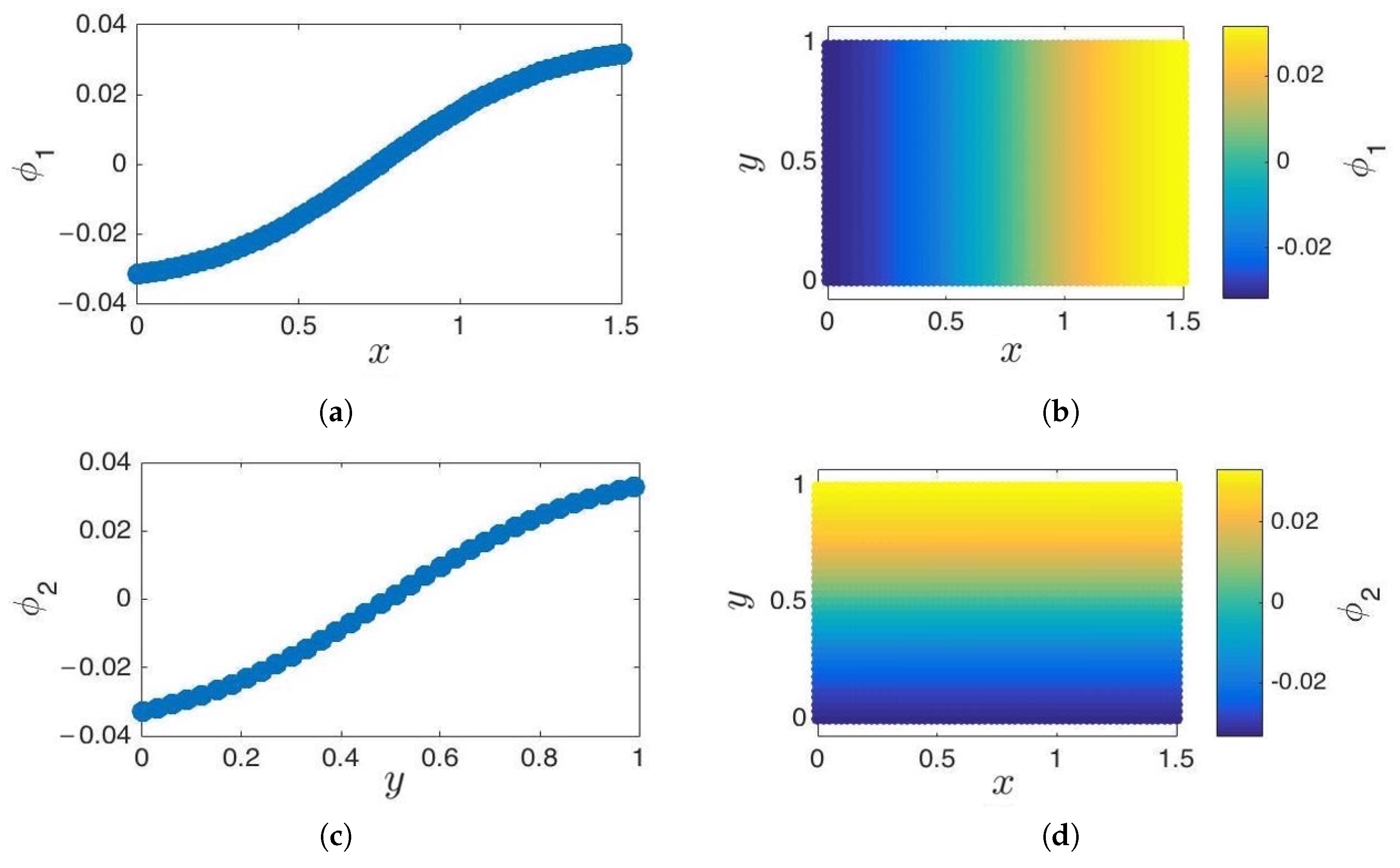
The independent eigenfunctions, φ 1 , 0 and φ 0 , 1 , are one-to-one with x and y, respectively, and thereby parameterize the manifold Ω (see Figure 8). Note that the normal derivatives of the eigenfunctions vanish near the boundaries by construction [75]. Recall that in iMapD, we need to be able to extend the current set of point-samples to obtain new initial conditions for running subsequent trajectories. We do so by using an appropriate extrapolation scheme (such as geometric harmonics, to be discussed in Section 3.5).
Extrapolating directly in cosine-diffusion map space presents some difficulties. This is because the parameterization near the edges of the currently explored region is flat, and extending functions in the diffusion map coordinates gives rise to ambiguities [75]. One option to alleviate the potential zero-derivative issue of cosine-based diffusion maps is to move the singularity inside the manifold. This can be attained by extracting a sine-like parameterization (hence, “sine-diffusion maps”). By solving (8) with absorbing (Dirichlet) boundary conditions instead of reflecting (Neumann) boundary conditions, the resulting eigenfunctions are:
ψ k 1 , k 2 ( x , y ) = sin k 1 π x / L 1 sin k 2 π y / L 2 .
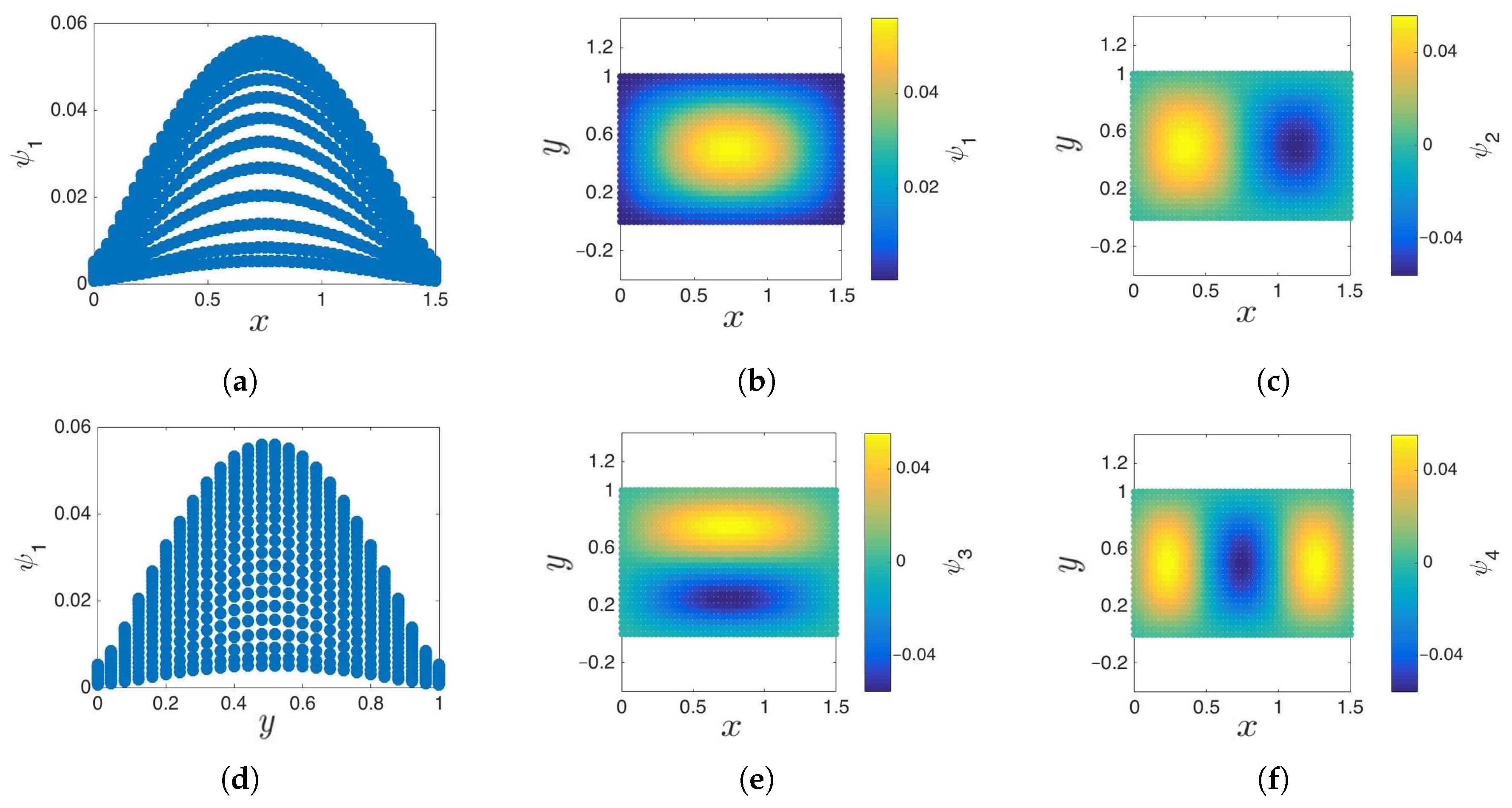
To approximate these eigenfunctions using the samples y 1 , , y m R n , we again construct the matrix W as we did for cosine-diffusion maps. Boundary detection algorithms are then used to locate the edge points. Absorbing boundary conditions are now imposed on the rows of these points: if y i is a boundary point, then the corresponding entry in the matrix W becomes W i j = δ i j . Alternatively, the boundary points can be duplicated, the matrix W constructed as in (6) and the rows and columns corresponding to a single set of boundary points then removed before obtaining W ˜ using (7). The eigendecomposition of W ˜ results in the eigenvectors, or sine-diffusion map coordinates, and their corresponding eigenvalues. These coordinates approximate the eigenfunctions (10). We can see on our 2D strip example (Figure 9) how the strip is colored by the sine-coordinates.
We make two observations. First, note that only the first nontrivial sine-coordinate is of importance: the subsequent eigenvectors are simply higher harmonics of the first. Because of this, the parameterization of a 2D nonlinear manifold can be accomplished with one sine-coordinate and one cosine-coordinate. Automatic detection of higher harmonics can be carried out in a variety of ways; here, we will just mention that we can accomplish this by studying the functional dependence between the eigenfunctions, and we refer the reader to the treatment in [76] (Section 2.1) for more details. In higher dimensions, the parameterization can be obtained by replacing the single cosine-coordinate (that is, the one that becomes almost constant around the point of interest) with a sine-based one. Second, for every sine-coordinate value and fixed x or y, there exist two potential data point candidates. This complicates the manifold parameterization and extrapolation scheme. Additionally, the data must be divided into groups, such that using the sine- and cosine-coordinates maintains a one-to-one relationship within the group.
To systematically determine which cosine-coordinate is poorly behaved for each boundary point, we examine the k-nearest neighbors of the point in question. The cosine-coordinate with the least variance among the neighbors is the one that should be replaced with the sine-coordinate. Parameterizing points using one sine-coordinate and one cosine-coordinate is not unique: for a fixed cosine-coordinate value, there are multiple points with the same sine-coordinate value. Therefore, care must be taken to maintain a one-to-one mapping throughout the entirety of the extrapolation.
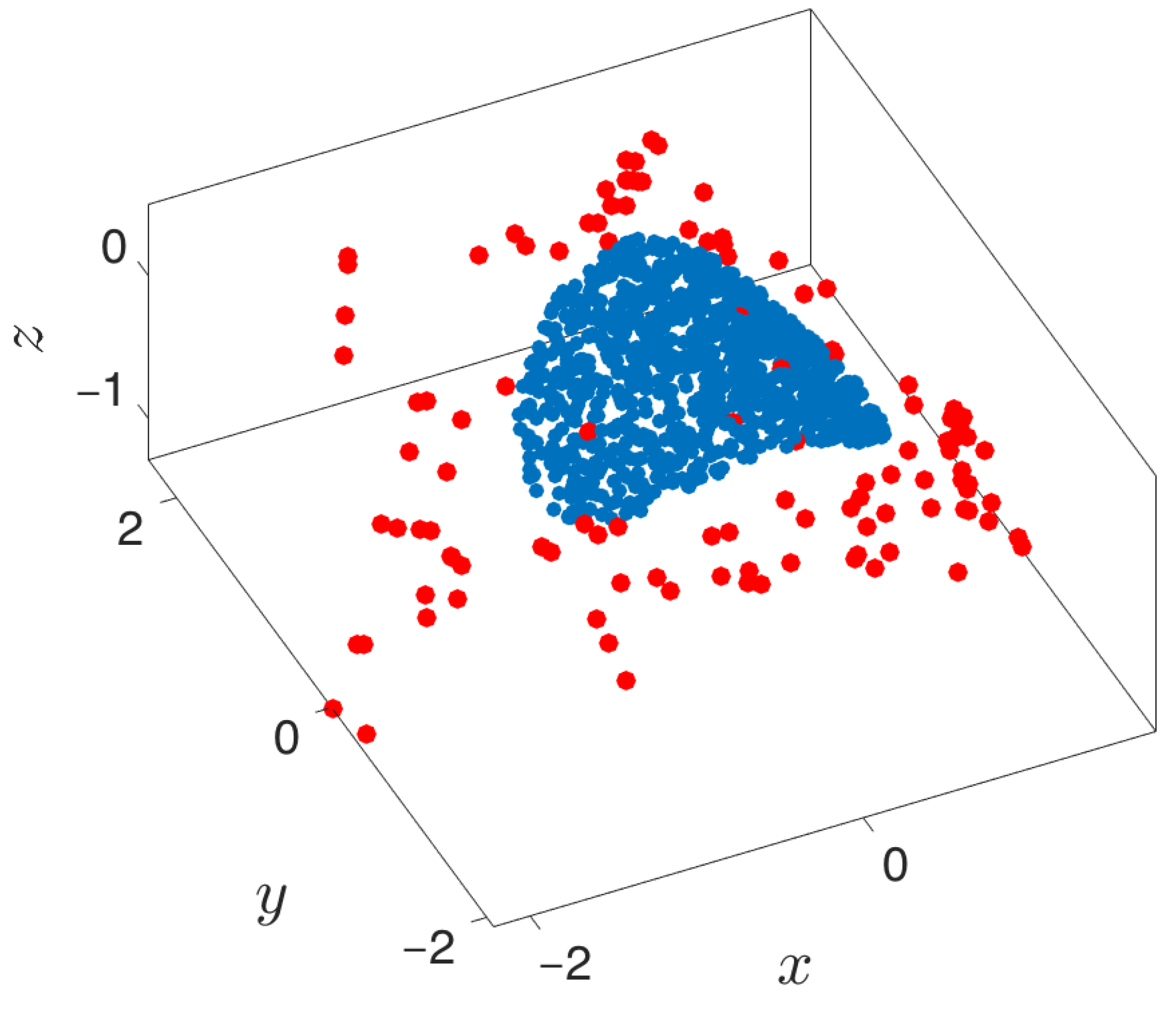
Once the data are divided into groups based on which cosine-coordinate to replace and the sign of its eigenvector, the boundary points can be extended and mapped to the original conformational space using the same techniques as for cosine-diffusion maps. A sample manifold extended via sine-diffusion maps with geometric harmonics is shown in Figure 10.

3.2. Local Principal Component Analysis

Rather than using DMAPS coupled with geometric harmonics, one could also use LPCA to extend the manifold. LPCA is simpler than DMAPS, but it requires a local set of collective variables for each boundary point rather than a single, global set of collective variables for the entirety of the data.
LPCA is based on PCA, a widely-used dimensionality reduction technique [77], which aims to find the best (in the least-squares sense) linear manifold that approximates a dataset. The method finds an orthogonal basis such that the first basis vector points in the direction of greatest variance and all subsequent vectors maximize variance in orthogonal directions. The basis vectors are known as principal components and are the linear counterpart of nonlinear diffusion coordinates. The first principal component describes the line of best fit through the data, the first two the plane of best fit, and so on.
Given m samples of n-dimensional data arranged in an n × m matrix X, we can find the principal components by first considering the matrix X ˜ , formed by mean-centering the data, and then computing the eigendecomposition of its covariance matrix, Y. The eigenvalues, sorted in descending order, determine the importance of each of the principal components, which are eigenvectors of Y. In practice, the principal components are found through the singular value decomposition of X ˜ T [78,79]. Indeed, X ˜ T = U Σ V T , and we have:
Y = X ˜ X ˜ T = U Σ V T T U Σ V T = V Σ U T U Σ V T = V Σ 2 V T .
Since Y is a symmetric and positive definite matrix, the SVD is equivalent to the eigenvalue decomposition, so the columns of V are the eigenvectors of Y, and the square of the singular values of X ˜ are the eigenvalues of Y. Each data point in X ˜ can be assigned a set of n principal scores, representing the projection of the point onto each principal component. This change of basis is accomplished via X ˜ V T X ˜ .
Dimensional reduction occurs when only the first k principal components are retained. The value of k is chosen by examining the interval spanned by the eigenvalues and locating the first spectral gap. Thus, the original high-dimensional, noisy data are mapped into k reduced dimensions via projection onto an appropriate linear subspace. While this technique works well for (almost) linear data, the attracting manifolds in the systems simulated with MD are typically nonlinear. Because of this, we restrict the use of PCA to small, local neighborhoods on the manifold that can be approximated as locally linear (provided that the potential of mean force is smooth). The combination of these local patches of PCA can serve as a form of nonlinear manifold learning, otherwise known as LPCA.
For use in the proposed exploration algorithm, we must first locate the edge points of the underlying manifold. Then, to obtain a reduced description, we can perform LPCA on small “patches” surrounding each boundary point [80,81]. Consider a single boundary point found with an appropriate boundary detection algorithm. Its k-nearest neighbors form a small neighborhood near the edge of the n-dimensional manifold. The outward normal of the manifold at this location can be approximated by locating the center of mass and creating a unit vector u from this center towards the current boundary point. By projecting u onto the linear subspace formed by the first n local principal components found by executing PCA on the neighborhood, we reduce potential noise, skewing the outward normal. The boundary point can be extended outward a given distance on this de-noised normal, thereby yielding the new initial condition to be used in the simulator. This process is repeated for each boundary point. Extension of a sample manifold using LPCA is shown in Figure 11.
Note that extended points within the manifold of Figure 11 correspond to the extension of boundary points that do not cleanly fall on the manifold edge. This is a shortcoming of the boundary detection algorithm rather than a problem of LPCA. However, LPCA is not without its own limitations. The underlying linearity assumption implies that the extension should be relatively short because the assumption will only hold in small neighborhoods of the boundary points. Further, boundary detection must be done in the (high-dimensional) conformational space unless another nonlinear manifold learning technique, like DMAPS, is used to reduce the entirety of the manifold to a few coarse variables. Finally, as LPCA produces a set of local coarse variables for each boundary point, book-keeping becomes increasingly complicated, especially as the entire exploration algorithm repeats LPCA for each expansion of the explored region. See [82] for an approach on handling the local charts.

3.3. Boundary Detection

The success of our proposed algorithm is contingent on the ability to identify the boundary of the set of samples collected so far in the metastable state being currently visited. There exist at least two types of boundary detection algorithms: methods to find the concave hull around the sampled points, that is the tightest piecewise linear surface that contains all of the points; and more general methods that attempt to appropriately classify all of the data points so as to determine which samples belong to the boundaries. For a d-dimensional manifold embedded in a higher, n-dimensional space, the edge is d 1 dimensional. Algorithms of the first type generate a d 1 dimensional polytope for data that are d-dimensional. Therefore, for practical detection of the boundary, these procedures should be applied to low-dimensional manifolds. Note, however, that in some instances, the boundary of the manifold in conformational space may not always be the same as the boundary of the manifold in DMAP space; we assume here that this is not the case. Algorithms of the second type can be performed in either the d or n-dimensional space and provide a more robust way to determine which points lie on the boundary of the manifold.
The first set of algorithms construct the concave hull of the dataset (an optimal polytope that contains all points while minimizing volume) and include, e.g., the swinging arm [83] and the k-nearest neighbors approach [84]. Both methods must be initialized at a point guaranteed to be on the boundary (such as the farthest point in a certain direction). In the 2D setting, the first method rotates a short line segment clockwise until a new point is hit, while the second method chooses from k-nearest neighbors the one that makes the widest angle. These procedures are then iterated until all of the boundary points in the dataset have been located. However, the produced concave hull can be different depending on which initial point is chosen.
In the alpha-shapes algorithm [85,86,87], two points are considered boundary points if there exists a disk (or sphere, in 3D) of user-specified radius α 1 in which (a) the points in question lie on the disk’s perimeter and (b) the disk contains no other points. In practice, this method is executed by computing the Delaunay triangulation. The alpha-shape is then the union of triangles whose circumradius is less than α 1 and the boundary points that comprise the alpha-shape [88]. Though this concave hull approach is computationally constrained to 3D, we utilize this method as MATLAB 2015 provides a built-in function. For higher dimensional manifolds, algorithms of the second class are appropriate. These methods iterate through each data point and use a set of parameters to determine whether on not they lie on the boundary [89,90,91,92].

3.4. Outward Extension across the Boundary of a Manifold

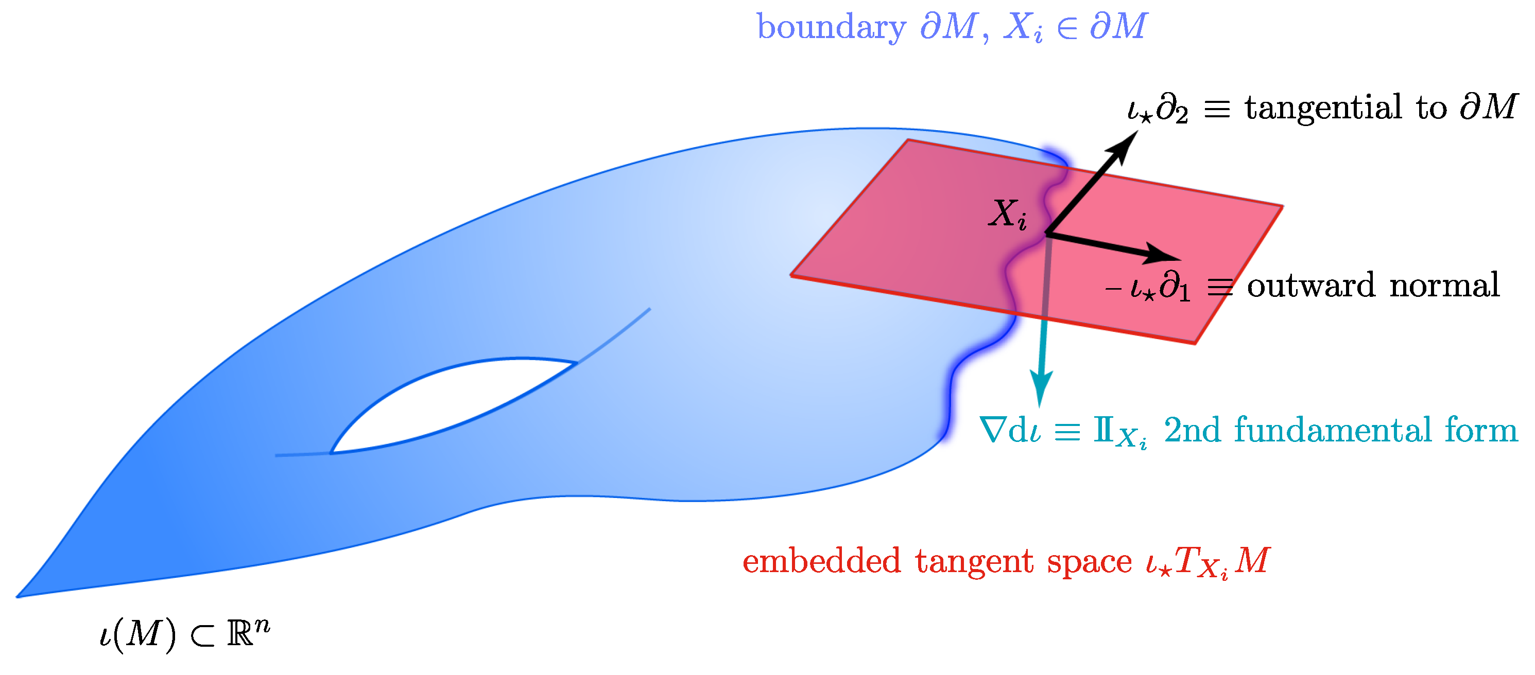
Let M be a smooth k-dimensional Riemannian manifold with a smooth boundary, M . The manifold M is isometrically embedded [93] in R n via the smooth mapping ι : M R n . We denote by ι the differential map (i.e., the Jacobian matrix at each point) associated with ι . It is well known [93] that ι maps tangent vectors of M into vectors in R n . In our case, ι is the embedding obtained via diffusion maps.
Consider the point x i M and its image X i = ι ( x i ) R n . The corresponding embedded tangent space ι T x i M has a natural basis ι 1 , , ι k , which is the image by ι of the canonical basis 1 , , k in a local chart around x i such that ι 1 is the inward normal at X i . This set of tangent vectors can be extended by an orthonormal frame e k + 1 , , e n R n such that ι 1 , , ι k , e k + 1 , , e n is a basis of R n ι T x i M × ( ι T x i M ) .
Let M ε = x M   |   d ( x , M ) ε ) , where d ( x , M ) denotes the geodesic distance from x M to the closest point in the boundary M . Let x M ε be such that x i is the closest point to x lying in M . Then, we define the reflective extension of X = ι ( x ) across the boundary of M, denoted by R ( x ) R p , as the vector:
R ( x ) = ι 1 , X X i   ι 1 + = 2 k ι , X X i   ι + = k + 1 n II X i e , X X i   II X i e ,
where · , · is the inner product associated with the Riemannian metric of M and II X is the second fundamental form [93] (Chapter 6), which describes how curved the embedded manifold is at a point X. Therefore, we can compute the outward extension of the point X as the new point X = X + δ R ( x ) R p for some δ > 0 (see also Figure 12).

3.5. Geometric Harmonics

In this section, we review the construction of geometric harmonics introduced in [94]. If we have a set of point-samples { y 1 , , y m } R n and a function f defined at those points, using geometric harmonics we can obtain an extension of f that is defined outside of the set of known samples. We will use geometric harmonics in Section 3.6 to fit a function to data and then extrapolate its value at new points.
Let us define the kernel:
w ( x , y ; ε 0 ) = exp x y 2 2   ε 0 ,
where x , y R n and ε 0 > 0 . Consider the symmetric m × m matrix W with elements W i j = w ( y i , y j ) . The matrix W is symmetric and, by Bochner’s theorem [95] (Theorem 6.10), Positive Semi-Definite (PSD). This implies that W has a full set of orthonormal vectors φ 1 , , φ m and its eigenvalues are real (due to W being symmetric) and non-negative (because W is PSD) λ 1 λ 2 λ m 0 .
For δ > 0 , let us consider the set S δ = { α   :   λ α > δ λ 1 } of indices of truncated eigenvalues. Let f be a function defined at some scattered points. We define the projection of f as:
f P δ f = α S δ f , φ α   φ α
with · , · being the inner product. The extension of P δ f evaluated at a point x { y 1 , , y m } is defined by:
( E f ) ( x ) = α S δ f , φ α   Φ α ( x ) where Φ α ( x ) = λ α 1 i = 1 m w ( x , y i ) φ i , α ,
where φ i , α is the i-th component of the eigenvector φ α . The functions Φ α are called geometric harmonics. By projecting and subsequently extending the function f, we have an effective method to evaluate the function at points outside the set of known point samples.
The accuracy of the extrapolation method described above depends on the relative error between f and its projection P δ f being bounded by η 0 (that is, whether f P δ f η f holds). In order to deal with functions where this condition is not satisfied, we use a multi-scale approach and project the residual f P δ f onto a finer scale, ε 1 = 2 1 ε 0 , by repeating the above procedure using a kernel w that uses ε 1 instead of ε 0 . This approach can be iterated by taking ε = 2 1 ε 0 for = 1 , 2 , until the norm of the residual is sufficiently small.
A complete treatment of geometric harmonics can be found in [94], and an application to chemical kinetics appears in [76] (Section 3.2.5). This scheme is a crucial component of lifting from diffusion map coordinates to conformational space coordinates, which constitute the functions to be extended.

3.6. iMapD Algorithm

The algorithm we propose performs a systematic search for unknown metastable states on the attracting manifold of a high-dimensional molecular system without a priori knowledge of coarse variables. The method relies on an external molecular dynamics package to numerically solve the equations of motion in (typically short) simulations, starting from a single set of initial conditions as input. There is also a number of problem-dependent algorithmic parameters (e.g., alpha shape parameters, extrapolation step lengths, etc.); the ones germane to iMapD are reported. The steps in the algorithm are detailed below:
  • Collection of an initial set of samples: The molecular system is initialized and evolved long enough so that it arrives at some basin of attraction. After removing the initial points that quickly arrive at the attracting manifold, the remaining data points constitute the initial set of samples (point cloud) on the manifold. These samples will be used in the subsequent steps of the method.
  • Parameterization of point cloud in lower dimensions: Using the set of samples from the previous step, we extract an optimal (and typically low-dimensional) set of coarse variables using DMAPS (for example, with cosine-diffusion maps). This process yields a parameterization of the local geometry of the free energy landscape around the region being currently visited by our system. All of our points are then mapped to the new set of coarse variables, thereby reducing the dimensionality of the system.
  • Outward extrapolation in low-dimensional space: After identifying the current generation of boundary points in the space of coarse variables (for example, via the alpha-shapes algorithm), we obtain additional points by extrapolating in the direction normal to the boundary.
  • Lifting of points from the (local) space of coarse variables to the conformational space: In order to continue the simulation, we must obtain a realization in conformational space of the newly-extended points in DMAP (or other reduced) space. In other words, we need a sufficient number of points in conformational space that are consistent with the DMAP (reduced) coordinates of the newly-extrapolated points. In the present paper, we use geometric harmonics, but in general, this task can be accomplished using biasing potentials, such as those available in PLUMED [96] or Colvars [97].
  • Repetition until the landscape is sufficiently explored: The lifted points serve as guesses for regions of the manifold that are yet to be probed. The system is reinitialized at these points (usually by running new parallel simulations), and the unexplored space is progressively discovered. This process is then repeated, effectively growing the set of sampled points on the free energy landscape.
In practice, this process begins with the initial simulation. The outcome is a set of samples within some basin of attraction that are then used in order to identify a few coarse variables via DMAPS. Once the points are mapped to the coarse variables, we run a boundary detection algorithm to identify points at the edges of the dataset. Then, for each boundary point p in DMAP space, the center of mass of its k-nearest neighbors is found. Each point is extended outward along the vector u connecting the center of mass to p. The new DMAP coordinates are then converted back into the conformational space. Using a training set of diffusion coordinates and their corresponding coordinates in the conformational space, geometric harmonics is used to fit the relevant function (e.g., a dihedral angle), extrapolate it to the newly-extended point and return approximate coordinates in conformational space for this new point. For the training set, we supply the nearest neighbors of the boundary point. Once each boundary point is extended and lifted to the conformational space, new simulations are initialized from these points. “Stitching” these new patches of explored regions together grows the approximation to the free energy landscape and explores it systematically without a priori knowledge of coarse variables.
In implementations of the algorithm, there arise various practical questions that affect the exploration of the attracting manifold, including:
  • Simulation run time: Though system dependent, simulations should be run until (a) the trajectory enters a region already explored, or (b) a new basin is discovered, or (c) a reasonable amount of time has passed for the trajectory to have explored “new ground” within the current basin. These conditions can be tested by detecting if the trajectory remains within a certain radius for a given amount of time (it has most likely found a potential well) or if the trajectory has a nontrivial amount of nearest neighbors from already explored regions.
  • Selection of trajectory points: Only “on manifold” points that belong to the basin of attraction should be collected. We implement this by removing a fixed number of points early in the trajectory that correspond to the initial approach to the attracting manifold. Discarding them will have the beneficial effect of preventing the exploration in directions orthogonal to the attractor. The exploration among the remaining points will lead to better sampling of basins and around saddle points within the attracting manifold.
  • Memory storage of data points: Observe that the samples gathered throughout the exploration process need not be kept in memory and can instead be stored in the hard drive. In principle, the file system or an appropriate database can be used to keep the corresponding files, but if storage space becomes an issue, then it is possible to randomly prune points whenever a (user-specified) maximum number of data points is exceeded. Note that if, between random pruning and preprocessing the data, distinct patches of explored regions appear, each sample of the manifold must be expanded separately so as not to discard samples that may have potentially reached new metastable states.

4. Conclusions

We have presented, illustrated and discussed several components of an algorithm for the exploration of effective free energy surfaces. The algorithm links machine learning (manifold learning, in particular, diffusion maps) with established simulation tools (e.g., molecular dynamics). The main idea is to discover, in a data-driven fashion, coordinates that parametrize the intrinsic geometry of the free energy surface and that can help usefully bias the simulation so that it does not revisit already explored basins, but rather extends in new, unexplored regimes. Smoothness and low-dimensionality of the effective free energy surface are the two main underpinning features of the algorithm. Its implementation involves several components (like point-cloud edge detection) that are the subject of current computer science research and has led to the development of certain “twists” in data mining (like the sine-diffusion maps presented here). We believe that such a data-driven approach holds promise for the parsimonious exploration of effective free energy surfaces. The algorithm is (in its current implementation) based on the assumption that the effective free energy surface retains its dimension throughout the computation. The systematic recognition of points at which this dimensionality may change and the classification of the ways this can occur are some of the areas of current research that could expand the scope and applicability of this new tool.

Acknowledgments

The work of Anastasia S. Georgiou, C. William Gear and Ioannis G. Kevrekidis was partially supported by the U.S. National Science Foundation and the U.S. Air Force Office of Scientific Research (F. Darema). Ioannis G. Kevrekidis was also partially supported through DARPA Contract HR0011-16-C0016. Eliodoro Chiavazzo acknowledges partial support of Italian Ministry of Education through the NANO-BRIDGE project (PRIN 2012, grant number 2012LHPSJC). We thank R. Covino and G. Hummer for many fruitful discussions and their collaboration.

Author Contributions

Eliodoro Chiavazzo and Ioannis G. Kevrekidis conceived of and designed the illustrative example computations, which were performed mainly by Anastasia S. Georgiou with Eliodoro Chiavazzo’s assistance. C. William Gear provided crucial insights in point cloud edge detection, as well as the development of sine-diffusion map algorithms. Hau-tieng Wu devised the differential geometric scheme for manifold extension. Juan M. Bello-Rivas wrote part of the paper, conducted the ABL1 protein analysis and integrated the remaining material with contributions from Eliodoro Chiavazzo and Ioannis G. Kevrekidis, as well as with input from all other authors. All authors have read and approved the final manuscript.

Conflicts of Interest

The authors declare no conflict of interest.

References

  1. Shaw, D.E.; Grossman, J.; Bank, J.A.; Batson, B.; Butts, J.A.; Chao, J.C.; Deneroff, M.M.; Dror, R.O.; Even, A.; Fenton, C.H.; et al. Anton 2: Raising the Bar for Performance and Programmability in a Special-Purpose Molecular Dynamics Supercomputer. In Proceedings of the SC14: International Conference for High Performance Computing, Networking, Storage and Analysis, New Orleans, LA, USA, 16–21 November 2014; pp. 41–53. [Google Scholar]
  2. Demir, O.; Ieong, P.U.; Amaro, R.E. Full-length p53 tetramer bound to DNA and its quaternary dynamics. Oncogene 2017, 36, 1451–1460. [Google Scholar] [CrossRef] [PubMed]
  3. Leimkuhler, B.; Matthews, C. Molecular Dynamics; Interdisciplinary Applied Mathematics; Springer International Publishing: Cham, Switzerland, 2015; Volume 39, pp. 1–88. [Google Scholar]
  4. Bryngelson, J.D.; Onuchic, J.N.; Socci, N.D.; Wolynes, P.G. Funnels, pathways, and the energy landscape of protein folding: A synthesis. Proteins 1995, 21, 167–195. [Google Scholar] [CrossRef] [PubMed]
  5. Wales, D. Energy Landscapes; Cambridge University Press: Cambridge, UK, 2004. [Google Scholar]
  6. Hamelberg, D.; Mongan, J.; McCammon, J.A. Accelerated molecular dynamics: A promising and efficient simulation method for biomolecules. J. Chem. Phys. 2004, 120, 11919–11929. [Google Scholar] [CrossRef] [PubMed]
  7. Darve, E.; Rodríguez-Gómez, D.; Pohorille, A. Adaptive biasing force method for scalar and vector free energy calculations. J. Chem. Phys. 2008, 128, 144120. [Google Scholar] [CrossRef] [PubMed]
  8. Hénin, J.; Fiorin, G.; Chipot, C.; Klein, M.L. Exploring multidimensional free energy landscapes using time-dependent biases on collective variables. J. Chem. Theory Comput. 2010, 6, 35–47. [Google Scholar] [CrossRef] [PubMed]
  9. Allen, R.J.; Valeriani, C.; Rein Ten Wolde, P. Forward flux sampling for rare event simulations. J. Phys. Condens. 2009, 21, 463102. [Google Scholar] [CrossRef] [PubMed]
  10. Roitberg, A.; Elber, R. Modeling side chains in peptides and proteins: Application of the locally enhanced sampling and the simulated annealing methods to find minimum energy conformations. J. Chem. Phys. 1991, 95, 9277–9287. [Google Scholar] [CrossRef]
  11. Krivov, S.V.; Karplus, M. Hidden complexity of free energy surfaces for peptide (protein) folding. Proc. Natl. Acad. Sci. USA 2004, 101, 14766–14770. [Google Scholar] [CrossRef] [PubMed]
  12. Schultheis, V.; Hirschberger, T.; Carstens, H.; Tavan, P. Extracting Markov Models of Peptide Conformational Dynamics from Simulation Data. J. Chem. Theory Comput. 2005, 1, 515–526. [Google Scholar] [CrossRef] [PubMed]
  13. Muff, S.; Caflisch, A. Kinetic analysis of molecular dynamics simulations reveals changes in the denatured state and switch of folding pathways upon single-point mutation of a β-sheet miniprotein. Proteins Struct. Funct. Bioinform. 2007, 70, 1185–1195. [Google Scholar] [CrossRef] [PubMed]
  14. Pan, A.C.; Roux, B. Building Markov state models along pathways to determine free energies and rates of transitions. J. Chem. Phys. 2008, 129, 064107. [Google Scholar] [CrossRef] [PubMed]
  15. Schütte, C.; Sarich, M. Metastability and Markov State Models in Molecular Dynamics: Courant Lecture Notes; American Mathematical Society: Providence, RI, USA, 2013; Volume 24. [Google Scholar]
  16. Laio, A.; Gervasio, F.L. Metadynamics: A method to simulate rare events and reconstruct the free energy in biophysics, chemistry and material science. Rep. Prog. Phys. 2008, 71, 126601. [Google Scholar] [CrossRef]
  17. Valsson, O.; Tiwary, P.; Parrinello, M. Enhancing Important Fluctuations: Rare Events and Metadynamics from a Conceptual Viewpoint. Ann. Rev. Phys. Chem. 2016, 67, 159–184. [Google Scholar] [CrossRef] [PubMed]
  18. Faradjian, A.K.; Elber, R. Computing time scales from reaction coordinates by milestoning. J. Chem. Phys. 2004, 120, 10880–10889. [Google Scholar] [CrossRef] [PubMed]
  19. Bello-Rivas, J.M.; Elber, R. Exact milestoning. J. Chem. Phys. 2015, 142, 094102. [Google Scholar] [CrossRef] [PubMed]
  20. Jónsson, H.; Mills, G.; Jacobsen, K.W. Nudged elastic band method for finding minimum energy paths of transitions. In Classical and Quantum Dynamics in Condensed Phase Simulations; World Scientific: Singapore, 1998; pp. 385–404. [Google Scholar]
  21. Mills, G.; Jónsson, H.; Schenter, G.K. Reversible work transition state theory: Application to dissociative adsorption of hydrogen. Surf. Sci. 1995, 324, 305–337. [Google Scholar] [CrossRef]
  22. Mills, G.; Jónsson, H. Quantum and thermal effects in H2 dissociative adsorption: Evaluation of free energy barriers in multidimensional quantum systems. Phys. Rev. Lett. 1994, 72, 1124–1127. [Google Scholar] [CrossRef] [PubMed]
  23. Sugita, Y.; Okamoto, Y. Replica-exchange molecular dynamics method for protein folding. Chem. Phys. Lett. 1999, 314, 141–151. [Google Scholar] [CrossRef]
  24. Lyubartsev, A.P.; Martsinovski, A.A.; Shevkunov, S.V.; Vorontsov-Velyaminov, P.N. New approach to Monte Carlo calculation of the free energy: Method of expanded ensembles. J. Chem. Phys. 1992, 96, 1776–1783. [Google Scholar] [CrossRef]
  25. Marinari, E.; Parisi, G. Simulated Tempering: A New Monte Carlo Scheme. Europhys. Lett. 1992, 19, 451–458. [Google Scholar] [CrossRef]
  26. Izrailev, S.; Stepaniants, S.; Isralewitz, B.; Kosztin, D.; Lu, H.; Molnar, F.; Wriggers, W.; Schulten, K. Steered Molecular Dynamics. In Computational Molecular Dynamics: Challenges, Methods, Ideas; Deuflhard, P., Hermans, J., Leimkuhler, B., Mark, A.E., Reich, S., Skeel, R.D., Eds.; Springer: Berlin/Heidelberg, Germany, 1999; pp. 39–65. [Google Scholar]
  27. Weinan, E.; Ren, W.; Vanden-Eijnden, E. String method for the study of rare events. Phys. Rev. B 2002, 66, 052301. [Google Scholar]
  28. Maragliano, L.; Fischer, A.; Vanden-Eijnden, E.; Ciccotti, G. String method in collective variables: Minimum free energy paths and isocommittor surfaces. J. Chem. Phys. 2006, 125, 024106. [Google Scholar] [CrossRef] [PubMed]
  29. Dellago, C.; Bolhuis, P.G.; Chandler, D. Efficient transition path sampling: Application to Lennard-Jones cluster rearrangements. J. Chem. Phys. 1998, 108, 9236–9245. [Google Scholar] [CrossRef]
  30. Bolhuis, P.G.; Chandler, D.; Dellago, C.; Geissler, P.L. Transition path sampling: Throwing ropes over rough nountain passes, in the dark. Ann. Rev. Phys. Chem. 2002, 53, 291–318. [Google Scholar] [CrossRef] [PubMed]
  31. Van Erp, T.S.; Moroni, D.; Bolhuis, P.G. A novel path sampling method for the calculation of rate constants. J. Chem. Phys. 2003, 118, 7762–7774. [Google Scholar] [CrossRef]
  32. Torrie, G.M.; Valleau, J.P. Monte Carlo free energy estimates using non-Boltzmann sampling: Application to the sub-critical Lennard-Jones fluid. Chem. Phys. Lett. 1974, 28, 578–581. [Google Scholar] [CrossRef]
  33. Kästner, J. Umbrella sampling. Wiley Interdiscip. Rev. Comput. Mol. Sci. 2011, 1, 932–942. [Google Scholar] [CrossRef]
  34. Huber, G.; Kim, S. Weighted-ensemble Brownian dynamics simulations for protein association reactions. Biophys. J. 1996, 70, 97–110. [Google Scholar] [CrossRef]
  35. Suárez, E.; Pratt, A.J.; Chong, L.T.; Zuckerman, D.M. Estimating first-passage time distributions from weighted ensemble simulations and non-Markovian analyses. Protein Sci. 2016, 25, 67–78. [Google Scholar] [CrossRef] [PubMed]
  36. Bernardi, R.C.; Melo, M.C.; Schulten, K. Enhanced sampling techniques in molecular dynamics simulations of biological systems. Biochim. Biophys. Acta 2015, 1850, 872–877. [Google Scholar] [CrossRef] [PubMed]
  37. Elber, R. Perspective: Computer simulations of long time dynamics. J. Chem. Phys. 2016, 144, 060901. [Google Scholar] [CrossRef] [PubMed]
  38. Peters, B. Reaction Coordinates and Mechanistic Hypothesis Tests. Annu. Rev. Phys. Chem. 2016, 67, 669–690. [Google Scholar] [CrossRef] [PubMed]
  39. Du, R.; Pande, V.S.; Grosberg, A.Y.; Tanaka, T.; Shakhnovich, E.S. On the transition coordinate for protein folding. J. Chem. Phys. 1998, 108, 334–350. [Google Scholar] [CrossRef]
  40. Geissler, P.L.; Dellago, C.; Chandler, D. Kinetic Pathways of Ion Pair Dissociation in Water. J. Phys. Chem. B 1999, 103, 3706–3710. [Google Scholar] [CrossRef]
  41. Peters, B. Using the histogram test to quantify reaction coordinate error. J. Chem. Phys. 2006, 125, 241101. [Google Scholar] [CrossRef] [PubMed]
  42. Krivov, S.V. On Reaction Coordinate Optimality. J. Chem. Theory Comput. 2013, 9, 135–146. [Google Scholar] [CrossRef] [PubMed]
  43. Van Erp, T.S.; Moqadam, M.; Riccardi, E.; Lervik, A. Analyzing Complex Reaction Mechanisms Using Path Sampling. J. Chem. Theory Comput. 2016, 12, 5398–5410. [Google Scholar] [CrossRef] [PubMed]
  44. Socci, N.D.; Onuchic, J.N.; Wolynes, P.G.; Introduction, I. Diffusive dynamics of the reaction coordinate for protein folding funnels. J. Chem. Phys. 1996, 104, 5860. [Google Scholar] [CrossRef]
  45. Best, R.B.; Hummer, G. Coordinate-dependent diffusion in protein folding. Proc. Natl. Acad. Sci. USA 2010, 107, 1088–1093. [Google Scholar] [CrossRef] [PubMed]
  46. Zwanzig, R. Nonequilibrium Statistical Mechanics; Oxford University Press: New York, NY, USA, 2001. [Google Scholar]
  47. Lei, H.; Baker, N.; Li, X. Data-driven parameterization of the generalized Langevin equation. Proc. Natl. Acad. Sci. USA 2016, 113, 14183–14188. [Google Scholar] [CrossRef] [PubMed]
  48. Hijón, C.; Español, P.; Vanden-Eijnden, E.; Delgado-Buscalioni, R. Mori–Zwanzig formalism as a practical computational tool. Faraday Discuss. 2010, 144, 301–322. [Google Scholar] [CrossRef] [PubMed]
  49. Chiavazzo, E.; Covino, R.; Coifman, R.R.; Gear, C.W.; Georgiou, A.S.; Hummer, G.; Kevrekidis, I.G. Intrinsic Map Dynamics exploration for uncharted effective free-energy landscapes. Proc. Natl. Acad. Sci. USA 2017, in press. [Google Scholar] [CrossRef]
  50. Wales, D.J. Perspective: Insight into reaction coordinates and dynamics from the potential energy landscape. J. Chem. Phys. 2015, 142, 130901. [Google Scholar] [CrossRef] [PubMed]
  51. Karatzas, I.; Shreve, S.E. Brownian Motion and Stochastic Calculus: Graduate Texts in Mathematics; Springer: New York, NY, USA, 1998; Volume 113. [Google Scholar]
  52. Gardiner, C. Stochastic Methods, 4th ed.; Springer Series in Synergetics; Springer: Berlin/Heidelberg, Germany, 2009; p. xviii+447. [Google Scholar]
  53. Risken, H. The Fokker-Planck Equation, 2nd ed.; Springer Series in Synergetics; Springer: Berlin/Heidelberg, Germany, 1989; Volume 18, p. xiv+472. [Google Scholar]
  54. Coifman, R.R.; Kevrekidis, I.G.; Lafon, S.; Maggioni, M.; Nadler, B. Diffusion Maps, Reduction Coordinates, and Low Dimensional Representation of Stochastic Systems. Multiscale Model. Simul. 2008, 7, 842–864. [Google Scholar] [CrossRef]
  55. Brenner, S.C.; Scott, L.R. The Mathematical Theory of Finite Element Methods; Vol. 15, Texts in Applied Mathematics; Springer: New York, NY, USA, 2008. [Google Scholar]
  56. Singer, A. From graph to manifold Laplacian: The convergence rate. Appl. Comput. Harmon. Anal. 2006, 21, 128–134. [Google Scholar] [CrossRef]
  57. Singer, A.; Coifman, R.R. Non-linear independent component analysis with diffusion maps. Appl. Comput. Harmon. Anal. 2008, 25, 226–239. [Google Scholar] [CrossRef]
  58. Dsilva, C.J.; Talmon, R.; Coifman, R.R.; Kevrekidis, I.G. Parsimonious representation of nonlinear dynamical systems through manifold learning: A chemotaxis case study. Appl. Comput. Harmon. Anal. 2015, 1, 1–15. [Google Scholar] [CrossRef]
  59. Chung, F.R.K. Spectral Graph Theory; CBMS Regional Conference Series in Mathematics, Published for the Conference Board of the Mathematical Sciences; American Mathematical Society: Providence, RI, USA, 1997; Volume 92, p. xii+207. [Google Scholar]
  60. Nadler, B.; Lafon, S.; Coifman, R.R.; Kevrekidis, I.G. Diffusion maps, spectral clustering and reaction coordinates of dynamical systems. Appl. Comput. Harmon. Anal. 2006, 21, 113–127. [Google Scholar] [CrossRef]
  61. Leimkuhler, B.; Matthews, C. Rational Construction of Stochastic Numerical Methods for Molecular Sampling. Appl. Math. Res. Express 2013, 2013, 34–56. [Google Scholar] [CrossRef]
  62. Parton, D.L.; Grinaway, P.B.; Hanson, S.M.; Beauchamp, K.A.; Chodera, J.D. Ensembler: Enabling high-throughput molecular simulations at the superfamily scale. PLoS Comput. Biol. 2016, 12, 1–25. [Google Scholar] [CrossRef] [PubMed]
  63. Chodera, J.; Hanson, S. Microsecond Molecular Dynamics Simulation of Kinase Domain of The Human Tyrosine Kinase ABL1. Available online: https://figshare.com/articles/Microsecond_molecular_dynamics_simulation_of_kinase_domain_of_the_human_tyrosine_kinase_ABL1/4496795 (accessed on 9 May 2017).
  64. Beberg, A.L.; Ensign, D.L.; Jayachandran, G.; Khaliq, S.; Pande, V.S. Folding@home: Lessons from eight years of volunteer distributed computing. In Proceedings of the 2009 IEEE International Symposium on Parallel & Distributed Processing Symposium, Rome, Italy, 23–29 May 2009; pp. 1–8. [Google Scholar]
  65. Eastman, P.; Swails, J.; Chodera, J.D.; McGibbon, R.T.; Zhao, Y.; Beauchamp, K.A.; Wang, L.P.; Simmonett, A.C.; Harrigan, M.P.; Brooks, B.R.; et al. OpenMM 7: Rapid Development of High Performance Algorithms for Molecular Dynamics. bioRxiv 2016. [Google Scholar] [CrossRef]
  66. Lindorff-Larsen, K.; Piana, S.; Palmo, K.; Maragakis, P.; Klepeis, J.L.; Dror, R.O.; Shaw, D.E. Improved side-chain torsion potentials for the Amber ff99SB protein force field. Proteins Struct. Funct. Bioinform. 2010, 78, 1950–1958. [Google Scholar] [CrossRef] [PubMed]
  67. Jorgensen, W.L.; Chandrasekhar, J.; Madura, J.D.; Impey, R.W.; Klein, M.L. Comparison of simple potential functions for simulating liquid water. J. Chem. Phys. 1983, 79, 926–935. [Google Scholar] [CrossRef]
  68. Skeel, R.D.; Izaguirre, J.A. An impulse integrator for Langevin dynamics. Mol. Phys. 2002, 100, 3885–3891. [Google Scholar] [CrossRef]
  69. Melchionna, S. Design of quasisymplectic propagators for Langevin dynamics. J. Chem. Phys. 2007, 127, 044108. [Google Scholar] [CrossRef] [PubMed]
  70. Essmann, U.; Perera, L.; Berkowitz, M.L.; Darden, T.; Lee, H.; Pedersen, L.G. A smooth particle mesh Ewald method. J. Chem. Phys. 1995, 103, 8577. [Google Scholar] [CrossRef]
  71. Chow, K.H.; Ferguson, D.M. Isothermal-isobaric molecular dynamics simulations with Monte Carlo volume sampling. Comput. Phys. Commun. 1995, 91, 283–289. [Google Scholar] [CrossRef]
  72. Åqvist, J.; Wennerström, P.; Nervall, M.; Bjelic, S.; Brandsdal, B.O. Molecular dynamics simulations of water and biomolecules with a Monte Carlo constant pressure algorithm. Chem. Phys. Lett. 2004, 384, 288–294. [Google Scholar] [CrossRef]
  73. Milstein, G.N.; Tretyakov, M.V. Stochastic Numerics for Mathematical Physics; Scientific Computation; Springer: Berlin/Heidelberg, Germany, 2004; p. xx+594. [Google Scholar]
  74. Coifman, R.R.; Lafon, S.; Lee, A.B.; Maggioni, M.; Nadler, B.; Warner, F.; Zucker, S.W. Geometric diffusions as a tool for harmonic analysis and structure definition of data: diffusion maps. Proc. Natl. Acad. Sci. USA 2005, 102, 7426–7431. [Google Scholar] [CrossRef] [PubMed]
  75. Belkin, M.; Que, Q.; Wang, Y.; Zhou, X. Toward understanding complex spaces: Graph Laplacians on manifolds with singularities and boundaries. arXiv, 2012; arXiv:1211.6727. [Google Scholar]
  76. Chiavazzo, E.; Gear, C.W.; Dsilva, C.; Rabin, N.; Kevrekidis, I. Reduced Models in Chemical Kinetics via Nonlinear Data-Mining. Processes 2014, 2, 112–140. [Google Scholar] [CrossRef]
  77. Jolliffe, I.T. Principal Component Analysis, 2nd ed.; Springer Series in Statistics; Springer: New York, NY, USA, 2002; p. xxx+487. [Google Scholar]
  78. Trefethen, L.; Bau, D. Numerical Linear Algebra; Number 50; Society for Industrial Mathematics: Philadelphia, PA, USA, 1997. [Google Scholar]
  79. Kutz, J.N. Data-Driven Modeling & Scientific Computation: Methods for Complex Systems & Big Data; Oxford University Press, Inc.: New York, NY, USA, 2013. [Google Scholar]
  80. Singer, A.; Wu, H.T. Vector diffusion maps and the connection Laplacian. Commun. Pure Appl. Math. 2012, 65, 1067–1144. [Google Scholar] [CrossRef] [PubMed]
  81. Cheng, M.Y.; Wu, H.T. Local Linear Regression on Manifolds and Its Geometric Interpretation. J. Am. Stat. Assoc. 2013, 108, 1421–1434. [Google Scholar] [CrossRef]
  82. Hashemian, B.; Millán, D.; Arroyo, M. Charting molecular free-energy landscapes with an atlas of collective variables. J. Chem. Phys. 2016, 145, 174109. [Google Scholar] [CrossRef] [PubMed]
  83. Galton, A.; Duckham, M. What is the region occupied by a set of points? In Geographic Information Science: Proceedings of the 4th International Conference, GIScience 2006, Münster, Germany, 20–23 September 2006; Springer: Berlin/Heidelberg, Germany, 2006; pp. 81–98. [Google Scholar]
  84. Moreira, A.; Santos, M.Y. Concave Hull: A k-Nearest Neighbours Approach for the Computation of the Region Occupied by a Set of Points. In Proceedings of the 2nd International Conference on Computer Graphics Theory and Applications (GRAPP 2007), Barcelona, Spain, 8–11 March 2007; pp. 61–68. [Google Scholar]
  85. Edelsbrunner, H.; Kirkpatrick, D.; Seidel, R. On the shape of a set of points in the plane. IEEE Trans. Inf. Theory 1983, 29, 551–559. [Google Scholar] [CrossRef]
  86. Edelsbrunner, H.; Mücke, E.P. Three-dimensional alpha shapes. ACM Trans. Graph. 1994, 13, 43–72. [Google Scholar] [CrossRef]
  87. Edelsbrunner, H. Surface Reconstruction by Wrapping Finite Sets in Space. In Discrete & Computational Geometry; Springer: New York, NY, USA, 2003; Volume 25, pp. 379–404. [Google Scholar]
  88. The MathWorks. MATLAB Documentation (R2015b). Alpha Shape; The MathWorks Inc.: Natick, MA, USA, 2015. [Google Scholar]
  89. Xia, C.; Hsu, W.; Lee, M.L.; Ooi, B.C. BORDER: Efficient computation of boundary points. IEEE Trans. Knowl. Data Eng. 2006, 18, 289–303. [Google Scholar]
  90. Qiu, B.Z.; Yue, F.; Shen, J.Y. BRIM: An Efficient Boundary Points Detecting Algorithm. In Advances in Knowledge Discovery and Data Mining; Springer: Berlin/Heidelberg, Germany, 2007; pp. 761–768. [Google Scholar]
  91. Qiu, B.; Wang, S. A boundary detection algorithm of clusters based on dual threshold segmentation. In Proceedings of the 2011 Seventh International Conference on Computational Intelligence and Security, Sanya, China, 3–4 December 2011; pp. 1246–1250. [Google Scholar]
  92. Gear, C.W.; Chiavazzo, E.; Kevrekidis, I.G. Manifolds defined by points: Parameterizing and boundary detection (extended abstract). AIP Conf. Proc. 2016, 1738, 020005. [Google Scholar]
  93. Do Carmo, M.P. Riemannian Geometry; Mathematics: Theory & Applications; Birkhäuser Boston, Inc.: Boston, MA, USA, 1992; p. xiv+300. [Google Scholar]
  94. Coifman, R.R.; Lafon, S. Geometric harmonics: A novel tool for multiscale out-of-sample extension of empirical functions. Appl. Comput. Harmon. Anal. 2006, 21, 31–52. [Google Scholar] [CrossRef]
  95. Wendland, H. Scattered Data Approximation (Cambridge Monographs on Applied and Computational Mathematics); Cambridge University Press: Cambridge, UK, 2005; Volume 17, p. x+336. [Google Scholar]
  96. Tribello, G.A.; Bonomi, M.; Branduardi, D.; Camilloni, C.; Bussi, G. PLUMED 2: New feathers for an old bird. Comput. Phys. Commun. 2014, 185, 604–613. [Google Scholar] [CrossRef]
  97. Fiorin, G.; Klein, M.L.; Hénin, J. Using collective variables to drive molecular dynamics simulations. Mol. Phys. 2013, 111, 3345–3362. [Google Scholar] [CrossRef]
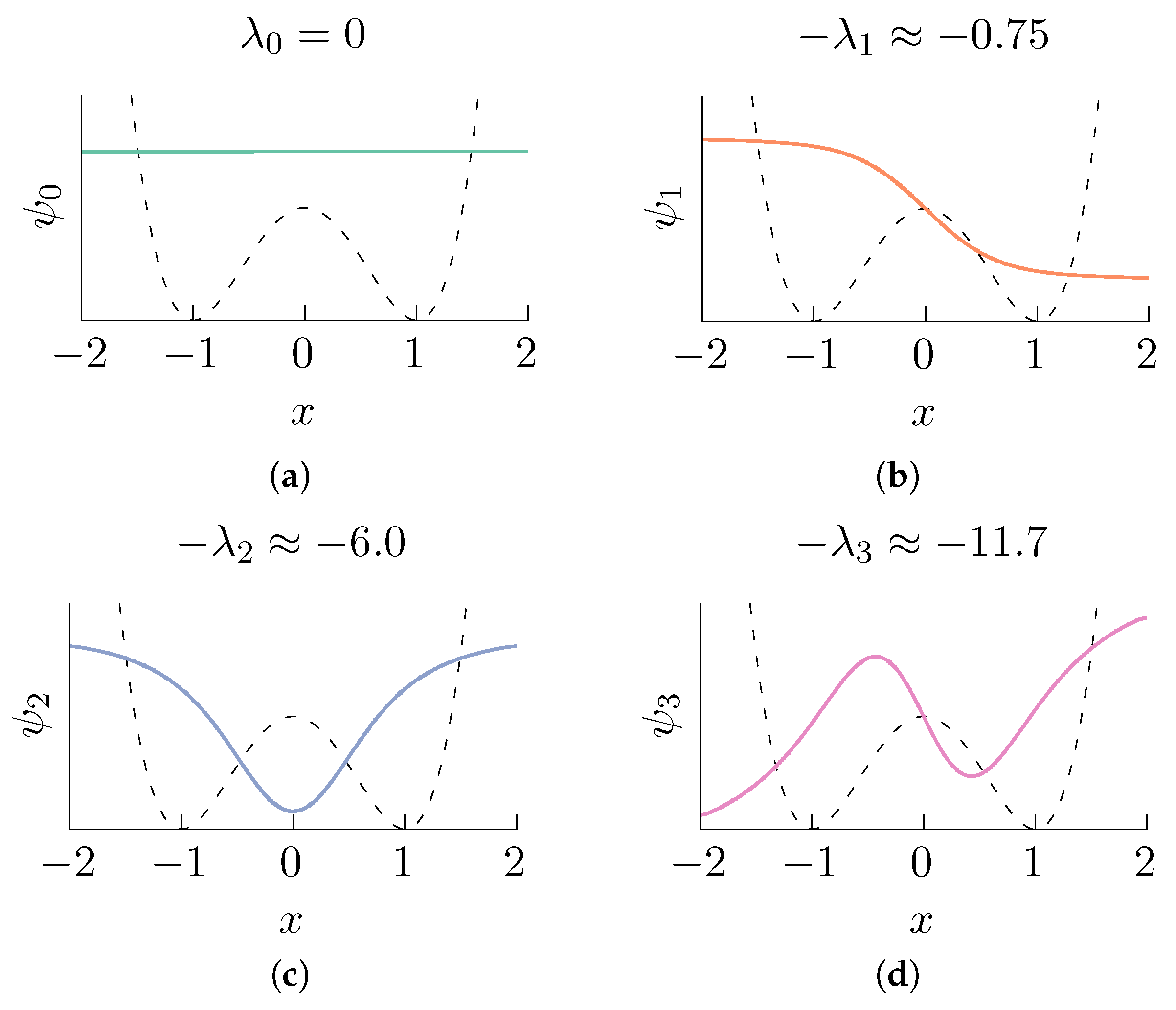
Figure 1. First eigenvalues and the corresponding eigenfunctions (represented by continuous lines) of the operator L corresponding to the double well potential U ( x ) = ( x 2 1 ) 2 (shown in the figure in dashed lines) at temperature β 1 = 1 . Observe that ψ 1 ( x ) is approximately an indicator function that attains its maximum at one energy well, its minimum at the other, and is invertible throughout the interval. The eigenfunctions were computed by numerically solving the eigenvalue problem associated with (3), and the solution was obtained using the finite element method [55] with quadratic Lagrange elements and meshing the interval [ 2 , 2 ] with 10 4 domain elements. (a) λ 0 = 0 ; (b) λ 1 0.75 ; (c) λ 2 6.0 ; (d) λ 3 11.7 .
Entropy 19 00294 g001
Figure 2. Data-driven computation of the right eigenvectors of the random walk Laplacian L obtained using a value of ε = 1 4 and a set of m = 10 3 data points (with inverse temperature β 1 = 1 ). Compare with Figure 1. We used the BAOAB integrator [61] (this is a fourth-order accurate numerical scheme for solving Brownian dynamics) in the high friction limit with a time step length of 10 4 to compute a numerical solution of (1) with initial condition x 0 = 1 . The numerical integration was carried out for a total of 10 8 steps retaining one every 10 5 points, and it was verified that the samples yield a sufficiently good approximation of the exact stationary distribution by ensuring that the total variation distance between the empirical and the exact distributions was below a threshold of 0.025 . Each subfigure corresponds to an eigenvalue: (a) λ 0 ; (b) λ 1 ; (c) λ 2 ; (d) λ 3 .
Entropy 19 00294 g002
Figure 3. Joint density plot of visited points mapped onto the first two diffusion map coordinates, ψ 1 and ψ 2 , obtained using ε = 0.075 on a trajectory containing 4000 snapshots of a one microsecond-long simulation of the catalytic domain of the human tyrosine protein kinase ABL1. The distances between the data points were computed using the root mean square deviation among the alpha carbons of different snapshots.
Entropy 19 00294 g003
Figure 4. Two particular conformations from the two local maxima shown in Figure 3. The system visits conformations around (a) during the first part of the simulation, and it stays near (b) during the second part.
Entropy 19 00294 g004
Figure 5. A trajectory “descends” from its initial condition onto the attracting manifold, the cylinder with radius R and axis y. On the manifold, the trajectory arrives at one of the metastable states that is near the middle of the cylinder at different values of θ . These metastable sets are depicted as the lightest colored areas.
Entropy 19 00294 g005
Figure 6. At each iteration, the algorithm extends the set of samples in the basin of attraction in order to better explore the underlying manifold and increase the likelihood of exiting the metastable state through one of the boundary points. The point cloud in conformational space is shown on the left, and the corresponding points in Diffusion Map (DMAP) space are displayed on the right. Green points represent the boundary of the so-far explored region. The system is reinitialized from the extended points, shown in magenta in both DMAP and conformational space. (a) The first iteration of the algorithm remains close to the basin of attraction. (b) The parameterization of the points formed by the first step in DMAP space. (c) The result of the third iteration of the algorithm in conformational space. (d) The result of the third iteration in DMAP space. (e) The result of the fifth iteration of the algorithm in conformational space. (f) The result of the fifth iteration in DMAP space. (g) By the seventh iteration, the point cloud escapes the initial basin of attraction. (h) The result of the seventh iteration in DMAP space.
Entropy 19 00294 g006
Figure 7. The goal of reaching the second metastable state is attained here at Step 11.
Entropy 19 00294 g007
Figure 8. Cosine-diffusion maps on a 2D strip. (a,b) The first diffusion coordinate, φ 1 , parameterizes the x direction. (c,d) The second diffusion coordinate, φ 2 , parameterizes the y direction. Functions are cosine-like, and their normal derivative vanishes on the edges. These functions approximate φ 1 , 0 and φ 0 , 1 , the eigenfunctions of the 2D Laplace–Beltrami operator with reflecting boundary conditions, respectively.
Entropy 19 00294 g008
Figure 9. Sine-diffusion map on a 2D plane. Solving the eigenproblem associated with the Laplace–Beltrami operator with absorbing boundary conditions results in diffusion coordinates with sine-like behavior. (a,b,d) Given a fixed x or y, the first sine-coordinate, ψ 1 , parameterizes y or x, respectively. (c,e,f) Subsequent eigenvectors ( ψ 2 , ψ 3 and ψ 4 ) are higher harmonics of the first.
Entropy 19 00294 g009
Figure 10. Extending and lifting using one sine-coordinate and one cosine-coordinate. Geometric harmonics is used as the lifting technique. Blue points represent the original point cloud, while red points depict the newly extended points.
Entropy 19 00294 g010
Figure 11. Extended manifolds using local PCA. Points extended into the manifold are a function of the boundary detection algorithm. Blue points represent the original point cloud, while red points depict the newly extended points.
Entropy 19 00294 g011
Figure 12. An illustration of M embedded in R n via ι and its relationship with the tangent space, the normal direction and the curvature.
Entropy 19 00294 g012
Table 1. Difference between maximum and minimum values of the azimuthal angle θ ( x , z ) for the point-cloud at different iterations. Since the attracting set is a cylinder, this measure tells us how much the size of the point-cloud expands as iterations proceed for a generic run of the simulation.
Iteration max θ min θ
00.36
10.55
20.75
30.99
41.21
51.49
61.76
72.00
82.25
92.60
102.95
113.33
123.49
133.98