1. Introduction
Mechanisms for chemical kinetics have steadily been developed during the last decades in order to improve predictions and reliability of combustion and fuel oxidation processes [
1]. This leads to a considerable increase in size (as number of species and reactions involved) and in stiffness of resulting mathematical models. In the same way, the dimension and complexity of the system has also been increased (hundreds of species and thousands of reactions with timescales covering more than 10 orders of magnitude [
1]). Large kinetic models require sophisticated integration software and enormous computational effort (e.g., Central Processing Unit (CPU) time, memory storage), making them inapplicable and inefficient for complex reacting flow simulations [
2]. This motivates the development of reduced models describing the combustion process with an acceptable accuracy but having significantly lower computational load [
3].
Today, a lot of different approaches have been developed to cope with this problem (see e.g., [
3] for a review of the developed methodologies). Although there is a substantial progress made in understanding and in development of sophisticated model reduction approaches, in applications, the mostly used methodology is still based on the concept of skeletal mechanisms [
4]. This is due to the simplicity of implementation and the intuitive nature of such an approach. It only needs to exclude reactions/species from the initial detailed mechanism, stating that the others are the only “important” for a considered application range. The main questions to be answered for the implementation of this method are: what is a suitable dimension of the chemical kinetic model (how many and which species should be considered?) and which reactions have to be included in the skeletal model. In order to answer these questions, many different concepts were introduced ranging from sensitivity analysis [
5], Level Of Importance (LOI) index [
6], Computational Singular Perturbation (CSP) pointers [
7] to mass flow and material flow analysis of the specially designed graph of chemical reaction network [
8].
An efficient method to find the important reactions and comprise a skeletal mechanism has been recently developed by Kooshkbaghi et al. [
9,
10]. In these studies, an entropy production was used to define which reactions contribute the most to the progress of combustion process. In this work, however, we use a combination of characteristic timescales and the entropy production analysis to cope with the problem of model reduction. Local characteristic timescales of chemical kinetics are calculated from the Jacobian matrix of the chemical source term [
11]. The corresponding chemical reaction modes/processes are quantified by the amount of entropy produced in the chemical process corresponding to different timescales. In this respect, the main objective of the current study is to investigate the multiple timescales of a reacting system, while the entropy production is used to quantify different modes of chemical reactions.
Theoretically, the use of the characteristic timescales allows the decomposition of the system into low-dimensional sub-systems [
11]. However, the absence of a clear gap between the eigenvalues (characteristic timescales) in a typical large reaction mechanism makes an asymptotic separation of the timescales problematic. The relative entropy production rate calculated as the entropy amount produced in each characteristic timescale divided by the total entropy production is suggested to overcome this difficulty identifying the relevant groups of characteristic timescales. These groups of timescales describe the contribution of dormant, relatively slow and fast processes, which can be explicitly decoupled and used to design the reduced model based on the timescale separation assumption. Thus, the suggested approach can be used to single out this important information for subsequent implementation of the timescale decomposition.
In order to verify the suggested approach, a reaction mechanism for the combustion of hydrogen/air mixtures [
12] consisting of 19 reactions among 9 species was employed to illustrate and test the proposed method. A methane/dimethyl ether reaction mechanism [
13] containing 578 reactions and 90 species was considered afterwards to validate the approach on a complicated combustion system. An auto-ignition problem is explored for a wide range of operating conditions (
p = 1−15 bar,
T = 900–1500 K and stoichiometric equivalence ratio of
ϕ = 1) using both combustion systems. The identification of significant characteristic timescales reveals a smaller number of so-called “active” modes, i.e., those contributing to the progress of chemical reaction, compared with the initial number of chemical reaction modes. These represent the relatively slow processes producing up to 99% of total entropy and comprise the subsystem that has to be integrated in time. The other timescales (quasi-conserved (slow) remain dormant and fast remain relaxed) can be calculated by using established implicit algebraic relations.
In this way, the reduced system can be integrated, but the implicit nature of the equations comprising the reduced model is difficult to implement generically for combustion system integration (see e.g., [
14]). Therefore, in order to be able to implement the reduced model, a suitable framework has to be found so that it can be represented in a proper and convenient way for applications. However, after the modes are classified, elementary reactions contributing to these modes can be identified and suggested to be used in the resulting skeletal mechanism. In this respect, skeletal models represent a very simple and generic framework to further illustrate and implement the analysis performed.
2. Mathematical Model
The auto-ignition problem in an isobaric and adiabatic combustion system is considered. The system’s state space is completely described by
where
h denotes enthalpy,
p is the pressure,
Yi are the species (
i = 1
, …, ns) mass fractions and
Mi the species molar masses. Then, the mathematical model can be written as:
where
F is the chemical reaction source term and
J denotes the Jacobian matrix of partial derivatives of the source term by species state variables [
1]. The chemical reaction source (
F) has two first zero components for enthalpy and pressure (adiabatic and isobaric combustion system is considered), while the source term for species specific mole numbers can be calculated as:
where
St (
ns ×
nr) represents the mechanism stoichiometry matrix constructed from the stoichiometric factors of each species in each elementary reaction and
R is the elementary reaction rate of each chemical reaction
[
1]. The molar-specific entropy of the mixture
S [J∙mol
−1⋅K
−1] is computed for every state along the system solution. For an isobaric reacting system the entropy is given by [
15]
with index
i running from 1 to the number of chemical species
ns.
si denotes the specific entropy of species
i,
R is the universal gas constant,
T the temperature,
P the pressure,
Pa the atmospheric pressure and
the mean molar mass. The specific entropy (
si) is temperature and composition dependent.
At any point of the system solution trajectory, the Jacobian can be presented in its canonical diagonal form
, where
is the diagonal matrix of the Jacobian’s eigenvalues and matrices
Z and
denote left (by columns) and right (by rows) eigenvalues of the Jacobian matrix shown below:
Analytically, the canonical form might degenerate for equal eigenvalues, the corresponding eigensubspace has less dimensions than the number of equal eigenvalues. However, numerically the case of the degenerate canonical form is almost absent. Moreover, typically all eigenvalues are complex, but different.
The next step is to define the amount of entropy produced within a certain characteristic time scale
ti = 1/|
λi|. For this purpose, the entropy produced in the course of chemical reaction (1) can be expressed as:
here the projection matrix
is used to project
F onto the eigenspace of a particular eigenvalue, e.g.,
with a very important property—they have to sum up to the Identity matrix:
In this way,
can be computed for each time step
ti and characteristic timescale
λi along the system’s evolution towards equilibrium:
In order to quantitatively estimate the active modes for any specified threshold, i.e.,
δ = 0.01 (1%), and, therefore, to find which characteristic timescales (chemical reaction mode) has to be accounted for, a relative entropy production was calculated:
Those eigenvalues having relatively larger absolute values, but not contributing to the progress of chemical reaction, can be excluded and treated as relaxed (they describe fast processes but always stay inactive). At the same time, those having smaller absolute values reflect quasi-conserved quantities relevant to dormant group of chemical reactions.
In order to define the contribution of a particular chemical reaction
Rl to the overall entropy production in “active” chemical reaction modes, a further use of the chemical reaction source term structure was employed by modifying the stoichiometry matrix (see e.g., Equation (1)) of the reaction mechanism. Namely, the following quantity was used to study the importance of a particular elementary reaction:
with
St denoting the mechanism’s stoichiometry matrix and
Stl the modified matrix (all columns except
l are zero) taking into account the specified particular elementary reaction. Finally, these values were normalized to the overall entropy production for every time step over the entire parameter range
The suggested mathematical model was implemented in a MATLAB code in combination with the program HOMREA for modelling homogeneous reacting systems [
12].
3. Results and Discussion
The results presented in this section were obtained from a constant-pressure adiabatic homogeneous reactor model for the calculation of entropy production as well as for ignition delay times and for species profiles calculations. For this purpose, HOMREA [
12] was employed. The further analysis (timescales and relative entropy production) was carried out in a post-processing MATLAB code, which is directly coupled with the simulation software HOMREA. The algorithm was implemented for several sets of initial conditions between the ranges:
p = 1−15 bar,
T = 800−1500 K and equivalence ratio of
ϕ = 1−10. For discussions below, examples based on simulations carried out for a stoichiometric equivalence ratio
ϕ = 1 will be presented. Note, however, similar results were observed for other sets of system parameters in the specific range mentioned before.
The approach presented in this study was developed for an automatic implementation to handle large detailed chemical kinetic mechanisms and to study and distinguish the processes governing the dynamics of combustion systems. However, at the beginning, in order to verify and illustrate the proposed approach, the Warnatz mechanism for the description of ignition processes in hydrogen/oxygen (H
2/O
2) mixtures [
12] was employed. The considered mechanism consists of only 19 reactions among 9 species and has been widely used by other authors in the past [
16,
17]. Although hydrogen reaction mechanisms are, in general, small compared to the ones describing the combustion and oxidation of higher hydrocarbons, the main implementation steps in the chemistry reduction and simplification can be clearly represented by using this comparatively simple example. Note, however, that results for a more complex example (CH
4/DME) are also shown below.
Once verified, the performance of the suggested approach for the mentioned model, a larger elementary reaction mechanism is considered. The polygeneration mechanism (PolyMech) [
13] is a C
1–C
4 detailed chemical kinetic model developed to predict ignition delay times and species profiles of methane (CH
4)/dimethyl ether (DME) mixtures in a wide range of conditions (fuel/air equivalence ratios from 1−15, pressures between 10–30 bar and 600–1500 K). The reaction mechanism consists of 578 elementary reactions among 90 species, from which 60 reactions and 17 species belong to the DME sub-mechanism. It has been validated against ignition delay times and species profiles from Rapid Compression Machine (RCM) and shock tube experimental data over the mentioned condition range [
13]. The model was developed for the simulation of polygeneration processes, in which the description of main products profiles like H
2, CO and C
2 (ethane, ethylene, acetylene) plays a significant role [
18].
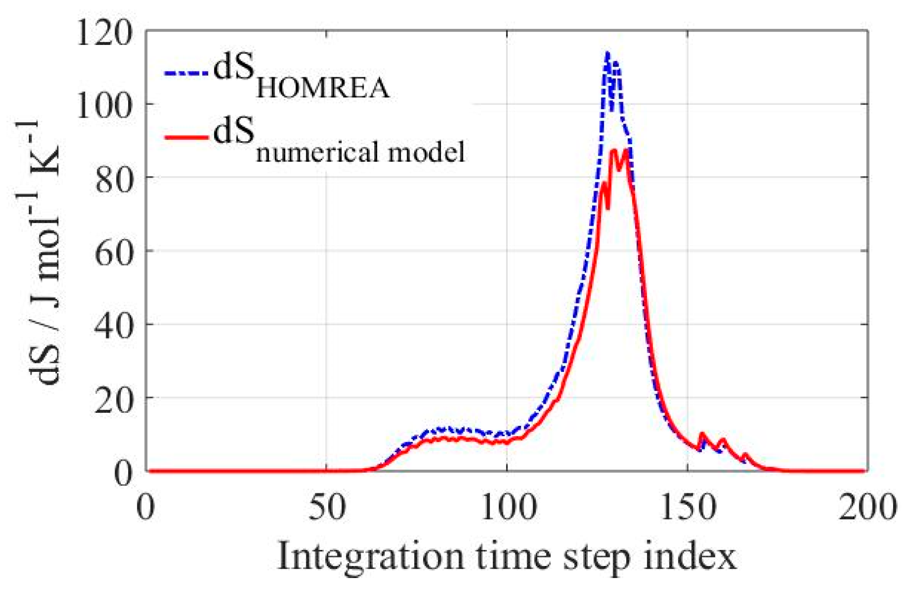
In order to start using the proposed mathematical model, a numerical value of the entropy production has to be calculated by using Equation (4). This calculated value will be implemented for further computations in combination with the projection matrix used to project the chemical reaction source term (
F) onto the eigenspace of a particular eigenvalue. The results obtained using Equation (4) were compared to the real entropy production of the system calculated by HOMREA and displayed in
Figure 1 for a H
2/O
2 mixture. Calculations of entropy production defined on the basis of timescale analysis Equation (4) implies the computation of the entropy variation with respect to all species
. This variation was approximated in the current version by:
where
denotes pseudo-inverse matrix. This approximation affects in a certain way the obtained values calculated with Equation (4) and therefore contributes to the discrepancy in the calculation of the entropy production observed in
Figure 1. Differences in the curves describing the numeric analysis and actual integrated entropy production are visible in
Figure 1. The discrepancy between both lies most likely in the discretization and explicit form of the entropy production definition used in Equation (4), including the approximation of the entropy variation with
expressed in Equation (9). Moreover, there is a numerical error in the eigenspace computations, especially for those eigenvalues having an imaginary part. In this case, the entropy produced is transformed into 2D real subspace and the outcome will be equally distributed between two conjugate eigenvalues. Therefore, differences are mainly observable in the initial stage of the ignition, where many complex eigenvalues are presented.
Local characteristic timescales obtained from the Jacobian-matrix eigenvalues (3) were calculated and sorted in ascending order by their absolute values at each time step. Once the simulations were concluded, the obtained eigenvalues were plotted against the integration time index in order to observe their evolution over time and be able to separate them in different groups of sub-processes. The decomposition of system timescales is generally characterized by a so-called gap between the timescales, which allows their division in different groups of modes. This methodology was, however, impossible to perform since in typical large combustion systems no gap between the eigenvalues is observed. The absence of a clear separation brought difficulties concerning the characteristic timescales separation. To overcome this problem, the suggested concept of relative entropy production was implemented. This can be calculated using Equation (6) as the entropy production of each timescale over the entire simulation time divided by the total entropy produced in the system. Thus, the entropy of irreversible multi-scale processes (e.g., detailed kinetic models) can be used to study the sub-space decomposition of the system (see e.g., Valorani et al. [
19]).
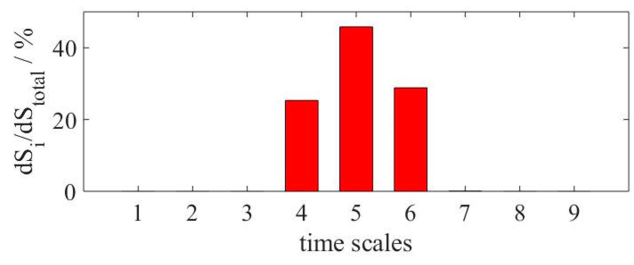
Figure 2 shows the time-integrated relative entropy production of the 9 timescales presented in the H
2 mechanism of Warnatz. A notable difference in the values calculated were observed. As mentioned before, a tolerance value of 1% (
δ = 0.01) was employed for computations using Equation (6). Since the difference between the relative entropy production values of each timescale is so pronounced, no tolerance variation analysis was performed. The results show that up to 99% of the system’s produced entropy is located within a relatively small group of eigenvalues (
λ4–
λ6), while the rest of them shown no contribution. The position of the timescales enables the identification of three groups of chemical reaction modes: dormant (
λ1–
λ3), relatively slow (
λ4–
λ6) and fast (
λ7–
λ9). The fast modes describe quickly relaxed processes, which in most of the cases remain stationary or quasi-stationary; the dormant ones are those that can be considered as quasi-conserved; and the relatively slow group of eigenvalues represent the processes that completely govern the progress of chemical reactions and are able to describe the dynamics of the corresponding system [
19].
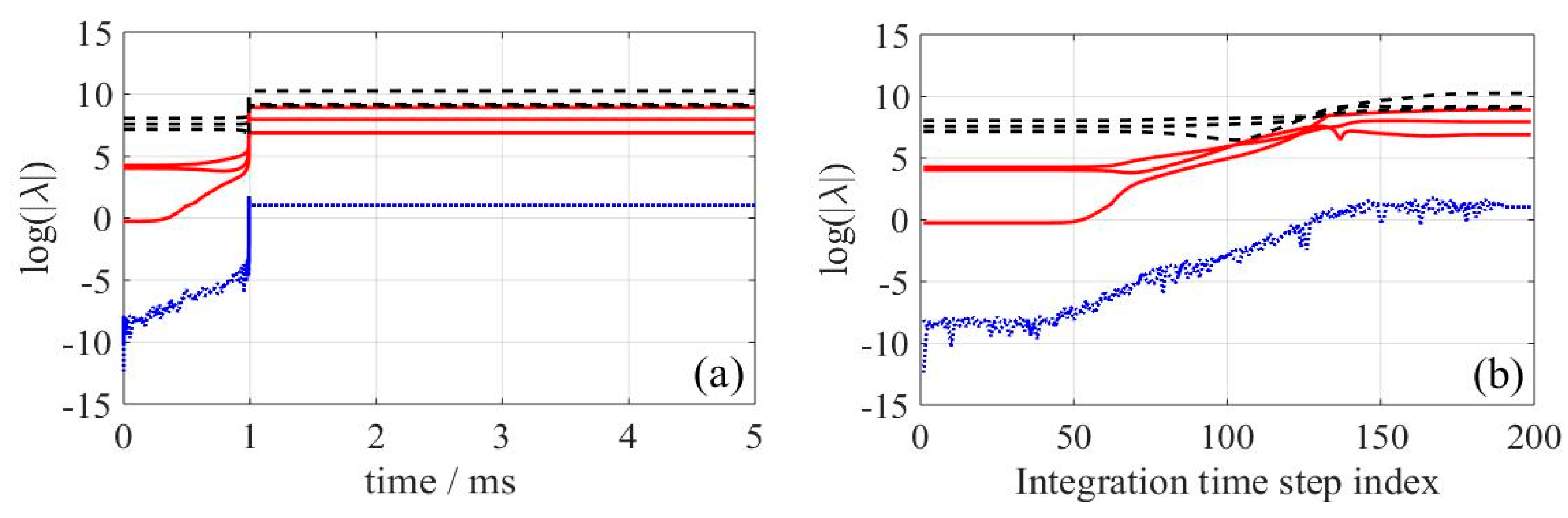
The decomposition of the system into three low-dimensional sub-systems becomes feasible by the implementation of the relative entropy production as a separation variable. The mentioned division of the system timescales are displayed in
Figure 3 for H
2/O
2 mixture. Each group is depicted with a different line format for an easier identification. Straight lines represent the timescales in which up to 99% of the system’s entropy is produced. These will be referred to as important or relevant in following descriptions. The number of timescales inside this sub-process group determines the overall dimension of the reduced system.
In
Figure 3, the logarithm of the system-eigenvalues in absolute values is depicted over the simulation time on the left (
Figure 3a) and over the integration time step index on the right (
Figure 3b). Time step index was preferred over the real simulation time since a better visualization of the system’s internal structure during reaction is possible. Changes of this function are considerable close to the ignition delay time, but almost negligible at the first milliseconds of reaction and near the equilibrium. As important events in combustion processes take place in a very short period of time, details will only be visible using integration time step index instead of the real simulation time as can be seen in
Figure 3a,b. The number of modes (i.e., characteristic timescales) located in each group of sub-processes depicted in
Figure 3 remains constant along the integration time. Namely, only three modes remain “active” and drive the system towards the equilibrium.
In this way, a real system dimension corresponding to the actual degrees of freedom is constituted as the number of processes that have to be determined in order to describe the progress of chemical kinetic reactions. The identification of the relevant characteristic timescales allowed a significant reduction of the system dimension (around 66%), lowering it from an initial value of 9 to a value of 3 after the conducted simplification method. The other two remaining groups of modes (dormant and quasi-stationary) can be solved by using implicit algebraic approximations. The implicit form of the reduced system can thus be expressed as:
where
,
and
are (
ni ×
n) matrices composed by
ni left eigenvectors corresponding to the related eigenvalues (see Equation (3)). In this case, the sub-index “
i” should be replaced by
f (fast),
s (slow) and
c (constant) depending on the algebraic approximation to solve in Equation (10). In order to implement the reduced model (10), an integration of the algebraic and differential equations (DAEs) of the system is needed. This is not the most convenient representation from a numerical point of view. Ordinary differential equation (ODE) systems are often preferable to DAE systems for solving this kind of problem.
It is well known that every timescale or chemical reaction mode represents a process that can be described by a set of reactions involved and responsible for the system’s progress and evolution [
7,
11]. Therefore, in the present work, the skeletal mechanism is constructed first as a simple way to transform the analysis results into an explicit representation of the reduced model. The group of important reactions can be identified by calculating the entropy production contribution of each reaction among the relevant characteristic timescales at each time step using Equations (7) and (8). Later on, these results are sorted in descending order by their absolute value. In this way, the most influential reactions can be identified by defining a value of delta (
δ) in Equation (8). The higher the value of
δ, the less the amount of reactions that will be selected.
The described procedure was repeated for all sets of conditions (temperature, pressure and equivalence ratio) implemented for the validation of the presented model as mentioned at the beginning of this section. The reactions selected as important for a particular set of physical parameters were written into an array, which gradually increased in size as the analysis was carried out for any other further temperature or pressure condition. This vector, containing all reactions selected, was used as input in an automatic reduction code. Reactions not presented in this final array, comprising all reactions contributing to the entropy production, were commented in the detailed mechanism. At present, there is no optimal criterion for the choice of the tolerance or delta. In the following, results using δ = 1% and 0.1% are displayed and compared. The higher the value of delta used in the analysis, the less reactions will be identified as important.
The reduced model obtained using the Warnatz mechanism [
12] for the combustion of hydrogen with
δ = 1% (highest value introduced) consisted of 14 reactions among 9 species. No reduction in terms of a number of species was observed, while 5 reactions less than in the original model were identified. Because of the small amount of species in the mechanism, no reduction in form of species number was expected, especially when considering that no modifications to reaction rates were performed. The results obtained are in accordance with the ones of other authors, which are mostly based in species and temperature sensitivity analysis for individual phenomena at lean to stoichiometric fuel/air equivalence ratios [
20,
21]. The hydrogen skeletal model obtained with the presented analysis and
δ = 1% matched almost perfectly the results when comparing with the ones of the detailed mechanism. Differences in the number of reactions by varying the value of delta from 1% to 0.1% were observed, but no significant discrepancy in the performance of the skeletal mechanism was observed.
The same procedure as for analysis in H
2/O
2 mixtures was carried out for methane/air combustion system described by the polygeneration mechanism (PolyMech) [
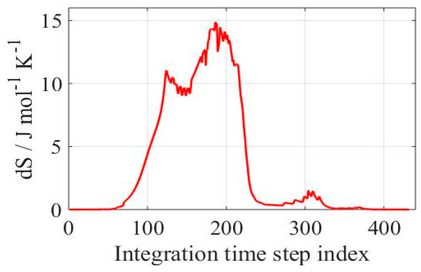
13]. The numerical entropy production using the PolyMech was calculated using Equation (4). The entropy produced by the system is displayed over the integration time step index for a CH
4/Air mixture in
Figure 4.
Figure 4 displays a typical time evolution of the entropy production for the considered system. The entropy production progress in
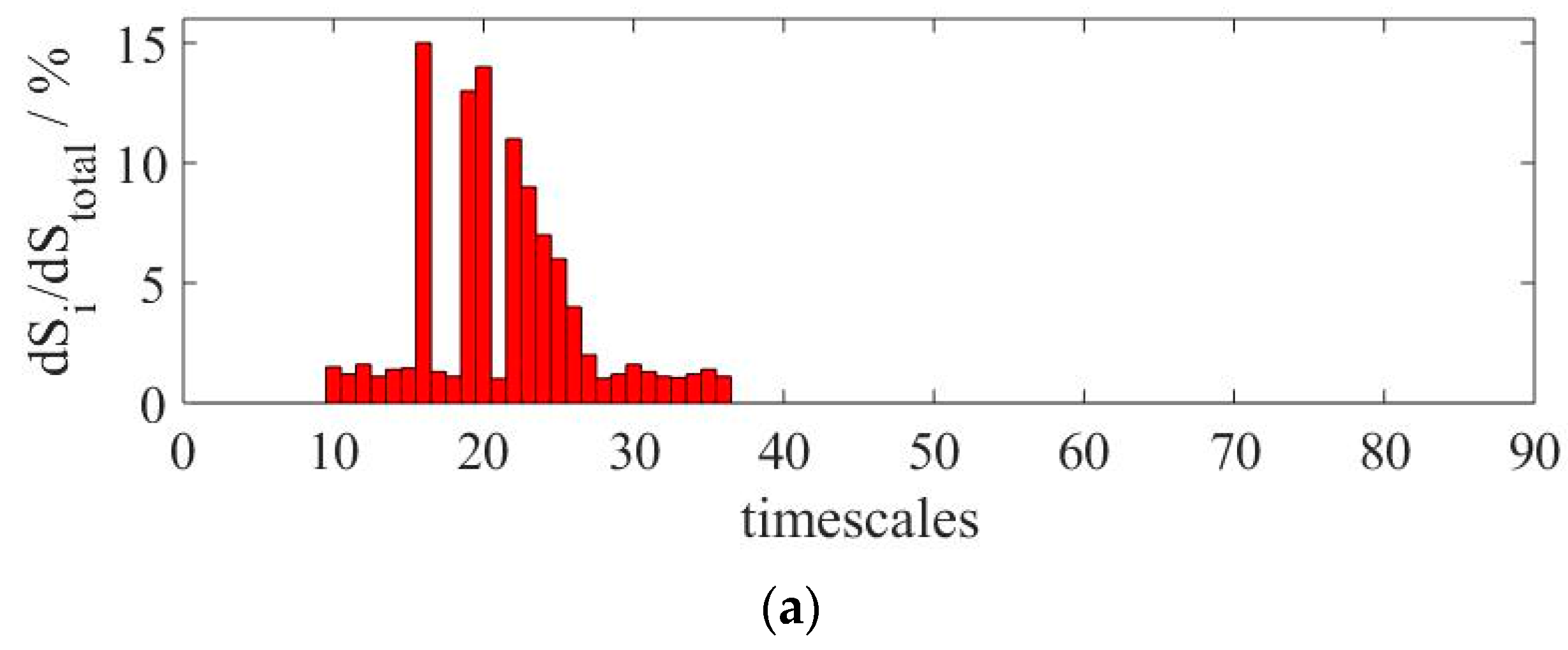
Figure 4 presents three local maxima: the first one corresponding to initiation reactions, a second for chain branching and propagation reactions and, finally, a relatively small local maximum for chain termination reactions. In order to decompose the dynamics of the system and identify the characteristic timescales governing the progress of chemical reactions, a relative entropy production rate was calculated using Equation (6). In this case, 26 characteristic timescales out of 90 were identified as important, as displayed in
Figure 5a. These represent the number of processes that have to be solved in order to describe the system dynamics. From the remaining timescales, 9 are located in the dormant group of sub-processes and 55 were identified as fast or quasi-stationary. The described division is depicted in
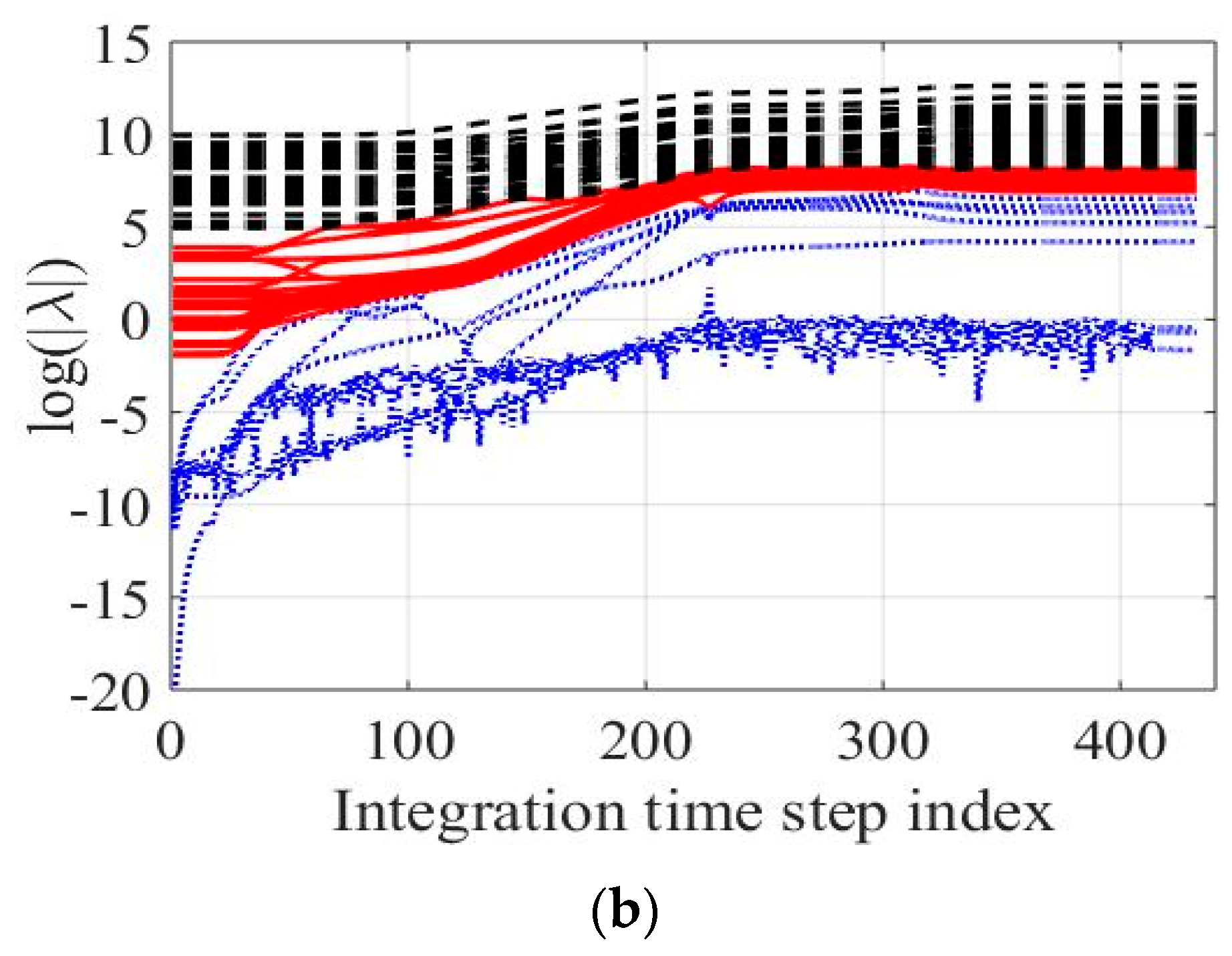
Figure 5.
Figure 5b shows the separation of the system timescales into the three groups of sub-processes identified above, also illustrated in
Figure 3 for a hydrogen/oxygen mixture, employing the PolyMech. The calculations were carried out for a CH
4/Air mixture at
T = 1100 K, 15 bar of pressure and stoichiometric equivalence ratios. As can be seen in
Figure 5, the system timescales are located closely together so no gap between them can be observed, disallowing a system decomposition without the use of the relative entropy production. The identification of the relevant characteristic timescales enabled also the determination of the reduced-system dimension, calculated from the number of timescales within the relative slow group, as mentioned before. For the considered case, a dimension reduction higher than 70% was obtained going from a value of 90 originally to
ns = 26 in the reduced model. The set of important reactions contained in the relative slow group of timescales was determined by comparing the amount of entropy produced by each reaction at each time step against the total amount of entropy produced at the considered time step (see Equation (8)). The value of delta was set to 1% and then changed to 0.1%, so two reduced versions of the same mechanism were obtained. The reduced version with
δ = 1% consists of 55 reactions among 30 species, while in the reduction with
δ = 0.1%, the number of reactions and species increased to 128 and 45 correspondingly.
Comparison of ignition delay times and species profiles using both skeletal mechanism versions and the detailed model were carried out in order to validate the first ones. The results obtained are displayed in
Figure 6,
Figure 7 and
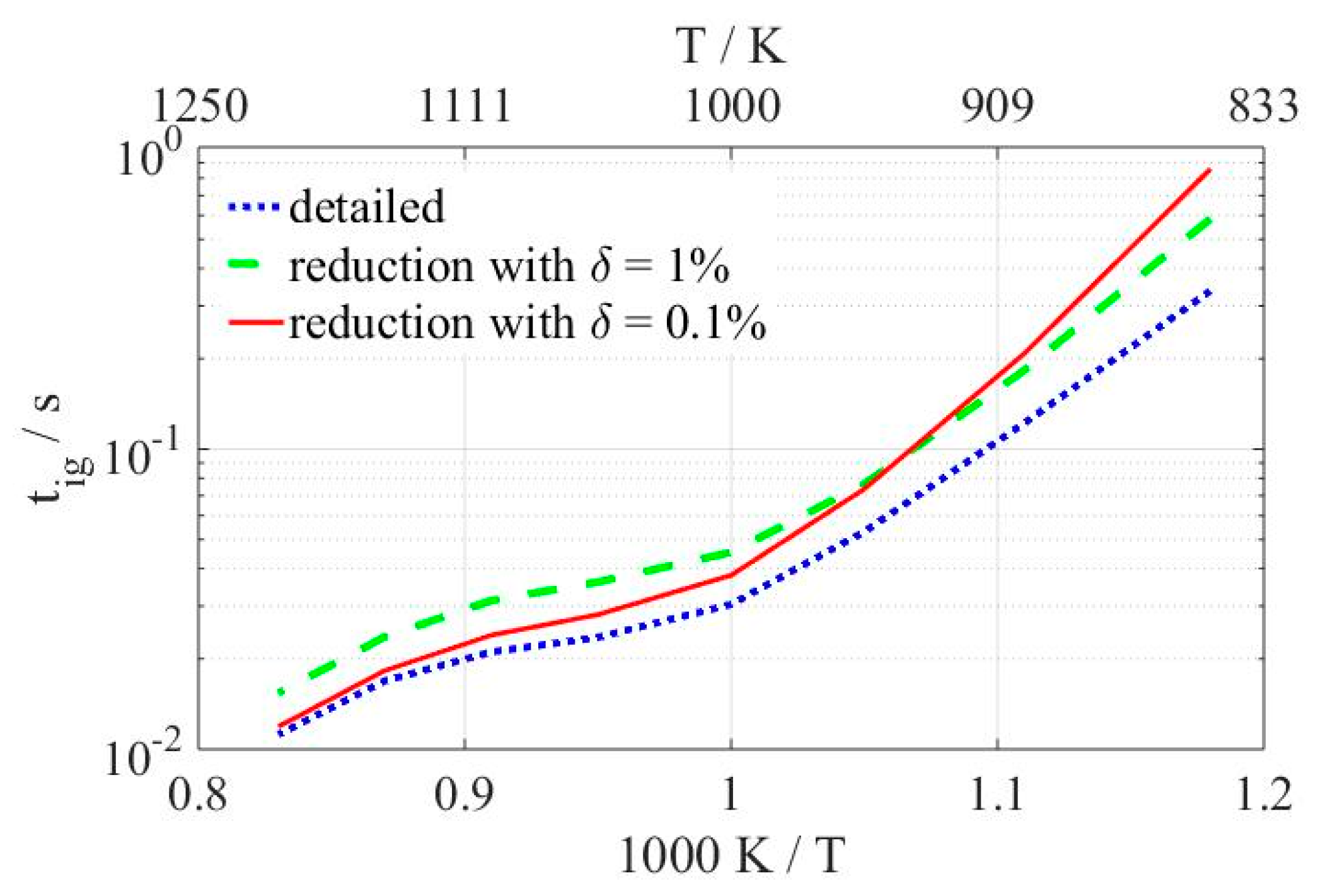
Figure 8. Ignition delay times (IDT), defined as the time at which the maximal molar composition of hydroxyl (OH) radical is reached, are compared in
Figure 6. Calculations were carried out for a temperature range of 850–1200 K and
p = 15 bar.
As can be seen in
Figure 6, none of the two skeletal mechanism match perfectly the curve representing the detailed model, both being slower than the latter one. The reduced model with
δ = 1% (dashed line) follows the same trend as the detailed model (dotted line). Meanwhile, the reduced version with
δ = 0.1% (straight line) lies significantly closer to the detailed mechanism at high temperatures and gradually moves away as the temperature decreases locating at higher values of IDT at temperatures below 930 K, the point at which the curves of both skeletal mechanisms intersect. IDTs of the model with the higher tolerance are, in average, by a factor 1.49 slower than the ones calculated with the detailed version of the PolyMech, while values obtained with the lower tolerance reduced model are, in average, in slightly better agreement with a factor of 1.42 with respect to the latter one.
Results of ignition delay times shown in
Figure 6 reveal a complex reaction network, where a higher number of reactions does not necessarily mean better accuracy and agreement of the results with respect to ignition delay times. The higher the number of reactions and species in the mechanism, the higher the complexity of the system to be analysed and solved. Further comparisons show the performance of the skeletal models with respect to species profiles. The same conditions used for calculations of ignition delay times (
p = 15 bar, stoichiometric equivalence ratio and
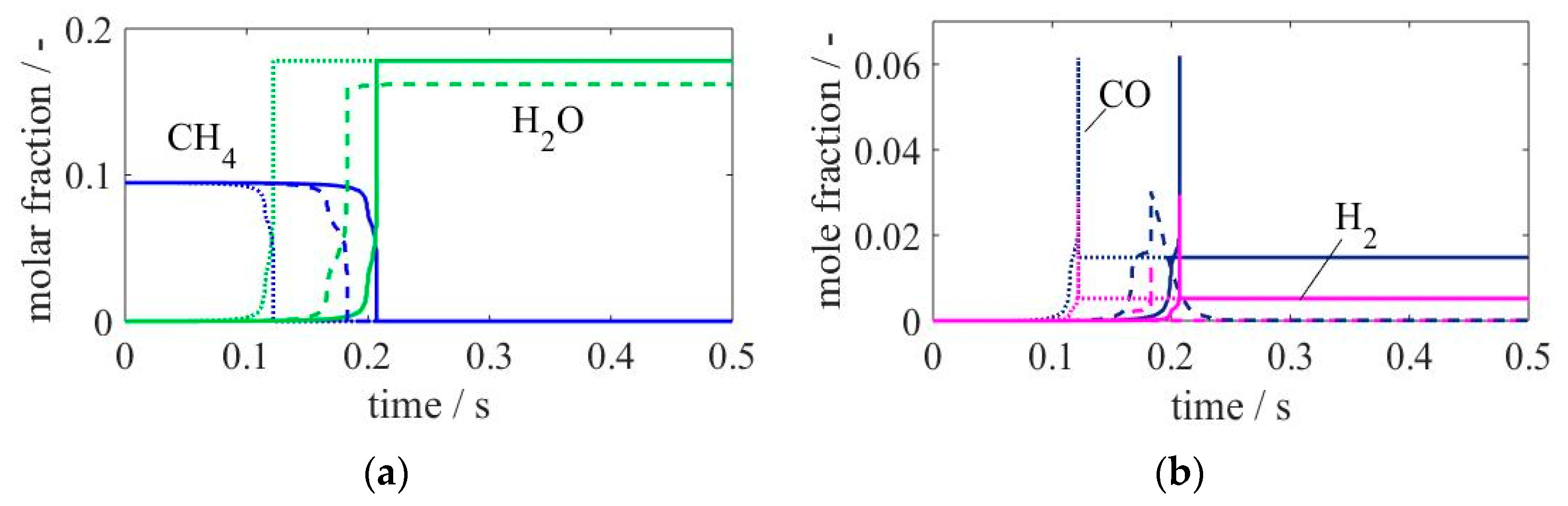
T = 900 K) were implemented in order to have a better overview of the reduced models performance. Results for methane (CH
4), water (H
2O), carbon monoxide (CO) and hydrogen (H
2) are displayed in
Figure 7.
Figure 7 shows species profiles of main products and reactants of the considered mixture. A shift in time is observed for all species in both reduced models. The model with
δ = 0.1% (straight lines) presents the slowest profiles, this being in accordance with the results observed in
Figure 6, since at the considered temperature (900 K), the reduced version with
δ = 1% presented faster IDTs. Though the profiles and therefore IDT are slower, the skeletal mechanism with
δ = 0.1% predicts the same product equilibrium composition as that obtained with the detailed model. The mentioned difference is notable on the water profile, where the equilibrium composition obtained using the reduced model with
δ = 1% is much lower, but even more remarkable for CO and H
2, where these species are produced and immediately completely consumed. A better and transparent visualization of the species profiles behaviour is possible when plotting these against the profile of another species as displayed in
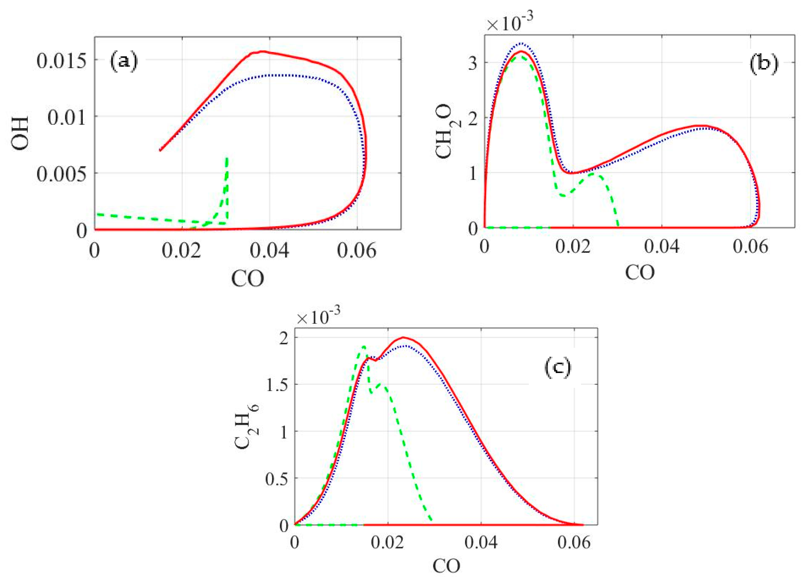
Figure 8.
In
Figure 8, mole fractions of some important products for further chemical applications, used as well as mechanism characteristic species in the combustion and oxidation of methane like OH (hydroxide radical), CH
2O (formaldehyde) and C
2H
6 (ethane), are plotted against the CO molar fraction for the same conditions used before in
Figure 7. As can be seen in
Figure 8, the molar composition relation of OH over CO is underestimated along the entire simulation time by the reduced model with
δ = 1%. Profiles of formaldehyde and ethane using the same reduced model are similar at the beginning to the ones obtained with the reduced model with
δ = 0.1% and the detailed model, but afterwards, the values are also under-predicted in both cases, being more notorious for CH
2O. The skeletal model with
δ = 0.1%, on the other hand, is in very good agreement with the profile relations of CH
2O and C
2H
6 when comparing to the results of the detailed mechanism. OH profiles calculated with this presents the same tendency as the detailed model but the production/consumption progress is slightly underestimated in most of the simulation time.
Since all reactions contained in the skeletal mechanism with δ = 1% are also contained in the reduced version with δ = 0.1%, differences and discrepancies observed between the two models are caused by those reactions (and species indirectly) representing only 1% of total entropy of the system. This means that some reactions with lower entropy production contributions have significant effects over the system behaviour.
Reactions involving the consumption/production of radicals or unstable species could have a very low contribution over the system’s entropy even when looking locally in time. Although these species could play an important role and be fundamental for the formation of other species with a higher entropy contribution.


