On the Configurational Entropy of Nanoscale Solutions for More Accurate Surface and Bulk Nano-Thermodynamic Calculations

Abstract

The configurational entropy of nanoscale solutions is discussed in this paper. As follows from the comparison of the exact equation of Boltzmann and its Stirling approximation (widely used for both macroscale and nanoscale solutions today), the latter significantly over-estimates the former for nano-phases and surface regions. On the other hand, the exact Boltzmann equation cannot be used for practical calculations, as it requires the calculation of the factorial of the number of atoms in a phase, and those factorials are such large numbers that they cannot be handled by commonly used computer codes. Herewith, a correction term is introduced in this paper to replace the Stirling approximation by the so-called “de Moivre approximation”. This new approximation is a continuous function of the number of atoms/molecules and the composition of the nano-solution. This correction becomes negligible for phases larger than 15 nm in diameter. However, the correction term does not cause mathematical difficulties, even if it is used for macro-phases. Using this correction, future nano-thermodynamic calculations will become more precise. Equations are worked out for both integral and partial configurational entropies of multi-component nano-solutions. The equations are correct only for nano-solutions, which contain at least a single atom of each component (below this concentration, there is no sense to make any calculations).

1. Introduction

Nanoscale technologies today are mostly empirical. They will be based on nanoscale science only if the validity of different scientific disciplines on which macroscale technologies are based are extended towards the nanoscale. One of those scientific disciplines is chemical thermodynamics, originally developed by Gibbs [1]. The classical validity of this discipline is restricted by the size of the phases in the system considered: it is classically valid only if all dimensions of all phases in a system are in the micro- or macroscale (above 100 nm), as in this case all molar Gibbs energies are size-independent quantities. However, if any of the phases in a system has at least one of its dimensions in the nanoscale (below 100 nm), the molar Gibbs energies and therefore phase equilibria will be size-dependent [2,3,4,5,6,7,8,9,10,11,12,13,14,15,16,17,18,19,20,21,22,23,24,25,26,27,28,29,30,31,32,33,34,35].

The majority of papers written so far on nanoscale phase equilibria discuss one-component systems [2,3,4,5,6,7,8,9,10,11,12,13,14,15] (see also references in these selected papers). A relatively small number of papers have been devoted to nanoscale phase equilibria of two-component systems [16,17,18,19,20,21,22,23,24,25,26,27,28,29,30,31,32,33,34,35]. For binary and multi-component solutions, the configurational entropy is one of the basic terms of the Gibbs energy of the solution phases, and thus its precise knowledge is crucial for nano-equilibrium calculations. The molar integral configurational entropy is usually written in the following form, obtained in the Stirling approximation ($S_{\mathrm{conf}}^{\mathrm{Stir}}$, J/mol·K) [36,37,38,39,40]:

$$S_{\mathrm{conf}}^{\mathrm{Stir}}\cong -R·{{\displaystyle \sum }}_{\mathrm{i}}{x}_i·\ln x_i$$

(1)

where $R$ = 8.3145 J/mol·K is the universal gas constant, $x_i$ (dimensionless) is the mole ratio of component i in the solution, defined as:

$$x_i\equiv \frac{N_{\mathrm{i}}}{{{\displaystyle \sum }}_i{N}_i}$$

(2)

where N_i is the number of atoms/molecules of component i in the solution. Equation (1) is routinely used in the thermodynamics of macroscale and microscale solutions [36,37,38,39,40]. It is also routinely used for nanoscale solutions in all papers devoted so far to phase equilibria in nanoscale binary solutions [16,17,18,19,20,21,22,23,24,25,26,27,28,29,30,31,32,33,34,35]. Thus, all previous papers on nano-thermodynamics neglected the difference between the actual value (after Boltzmann) and its Stirling approximation, being the subject of this paper.

As follows, Equation (1) is only an approximated equation, obtained by using the Stirling approximation [41,42] to the exact equation of Boltzmann [43,44]. This is done for two reasons: firstly, Equation (1) is much easier to use for practical calculations compared to the exact equation; secondly, the difference between the two is negligible for a large number of atoms/molecules of microscale and macroscale solutions. In the present paper, this difference will be studied for nanoscale solutions, and a correction term will be introduced as function of the number of atoms/molecules and the composition of nanoscale solutions.

2. The Exact Equation for the Integral Molar Configurational Entropy of Solutions

Entropy was defined in the most general way by Boltzmann [43,44] as:

$$S=k·\ln W$$

(3)

where k (J/K) is the Boltzmann constant (=R/N_Av, where N_Av is the Avogadro number), W (dimensionless) is the number of possible configurations of the atoms in the solution. Now, let us consider a binary solution made of N_A atoms/molecules A and N_B atoms/molecules B, with the total number of atoms/molecules: $N=N_{\mathrm{A}}+N_{\mathrm{B}}$. The A atoms/molecules are not distinguishable from each other, and the B atoms/molecules are not distinguishable from each other, either. Then, the number of possible configurations equals the number of multiset permutations:

$$W=\frac{N!}{N_{\mathrm{A}}!·N_{\mathrm{B}}!}$$

(4)

Now, let us substitute Equation (4) into Equation (3):

$$S=k·\ln \frac{N!}{N_{\mathrm{A}}!·N_{\mathrm{B}}!}$$

(5)

Now, let us convert Equation (5) into a molar integral configurational entropy by multiplying it with the ratio of the Avogadro number to the total number of atoms/molecules in the solution and remembering that $k·N_{\mathrm{Av}}=R$:

$$S_{\mathrm{conf}}=\frac{R}{N}·\ln \frac{N!}{N_{\mathrm{A}}!·N_B!}$$

(6)

Equation (6) is the exact equation for the molar integral configurational entropy of binary solutions ($S_{\mathrm{conf}}$, J/mol). It can be extended to n-component solutions as:

$$S_{\mathrm{conf}}=\frac{R}{N}·\ln \frac{N!}{{{\displaystyle \prod }}_i{N}_i!}$$

(7)

3. The Stirling Approximation for the Integral Molar Configurational Entropy of Solutions

Equation (6) is difficult to use, as the factorials of large numbers are so large that even computers refuse to calculate them (the Microsoft Office EXCEL 2007 software calculates the factorials to the maximum number of 170! = 7.3 × 10³⁰⁶, although other mathematical packages such as Maple or Mathematica are capable of handling the factorials of large numbers). Therefore, the Stirling approximation is usually applied, written as [41,42]:

$$\ln N!\cong N·\ln N-N$$

(8)

Now, let us replace both the $\ln N!$ and the $\ln N_i!$ terms in Equation (7) by Equation (8). After some re-arrangements, the approximated equation is obtained for the approximated integral molar configurational entropy of the solution, which is identical to Equation (1), if the mole fraction is defined by Equation (2).

Calculated results by Equations (1) and (6) are compared in Figure 1, Figure 2 and Figure 3. In Figure 2 and Figure 3 the relative error is shown, defined as:

$$error(\%)=100·\frac{S_{\mathrm{conf}}^{\mathrm{Stir}}-S_{\mathrm{conf}}}{S_{\mathrm{conf}}}$$

(9)

One can see that the Stirling approximation significantly deviates from the exact Boltzmann equation for low values of N—especially for non-equi-molar and for multi-component solutions. Although the relative error decreases with increasing the number of atoms in the phase, it is still too large for nano-Calphad calculations, even at N = 170 (the largest number for which we calculated the factorial using the Microsoft Office EXCEL 2007 software): this is 2.4% for binary equimolar solution, 4.3% for binary solution with 10 or 90 at % of the components (see Figure 2), and 3.8% for the equimolar, five-component solution (see Figure 3). It is especially critical when surface/interfacial thermodynamics is calculated, as the surface and interface regions contain much fewer atoms compared to bulk phases. That is why a new approximation is needed for more accurate nano-Calphad and surface/interface calculations.

4. Selection of the Optimum Approximation to Replace the Stirling Approximation

There are several new approximations for factorial expressions in the recent mathematical literature [45,46,47,48,49,50,51,52]. These approximations are different modified forms of the Stirling equation. However, all of them are so complex that their usage is not practical for the calculation of nano-equilibria. Let us rather go back to the 18th century, using the excellent book of Tweedle [42], which contains the original work of Stirling [41] and many useful commentaries. The equation in question was discussed by Stirling in his proposition 28, example 2. According to Tweedle, this equation of Stirling can be written in terms of natural logarithm as:

$$\ln N!\cong N·\ln \left(N+\frac{1}{2}\right)-\left(N+\frac{1}{2}\right)+\frac{1}{2}·\ln \left[2·\pi ·\left(N+\frac{1}{2}\right)\right]-\frac{1}{24·\left(N+\frac{1}{2}\right)}+\frac{7}{2880·{\left(N+\frac{1}{2}\right)}^3}+\dots$$

(10)

Although Equation (10) at first sight is quite different from Equation (8), it is true that Equation (10) becomes identical to Equation (8) at the limit of $N\to \infty$. Based on the correspondence between Stirling and de Moivre, soon after the publication of Equation (10), de Moivre published his own equation, which was somewhat different from Equation (10). According to Tweedle, the equation of de Moivre can be written as:

$$\ln N!\cong N·\ln N-N+\frac{1}{2}·\ln \left(2·\pi ·N\right)+\frac{1}{12·N}-\frac{1}{360·N^3}+\dots$$

(11)

Equations (10) and (11) provide similar numerical results, especially at relatively large N values. For practical purposes, however, Equation (11) is better than Equation (10), as its first two terms are exactly the same as those of the so-called “Stirling approximation” (Equation (8)). Thus, the de Moivre equation is more straightforward for use as the extended Stirling approximation. Now, the question is: how many terms of the de Moivre equation should be used for practical nano-Calphad calculations?

For nano-Calphad calculations, the region with $N<10$ is out of interest. Thus, we need a new approximation which will provide relative errors less than 0.1% at $N\ge 10$. The relative error of different combinations of terms of Equations (10) and (11) compared to the exact $\ln N!$ value is calculated for N = 10 in

Table 1. The relative errors (%) provided by different combinations of terms at N = 10 in Equations (10) and (11), compared to the exact value of $\ln N!$.

Term Numbers Combined	Equation (10)	Equation (11)
1	63.5	52.4
1 + 2	−6.06	13.03
1 + 2 + 3	0.026	−0.055
1 + 2 + 3 + 4	−1.39 × 10−5	−1.83 × 10−5
1 + 2 + 3 + 4 + 5	3.96 × 10−8	−5.21 × 10−8

. As follows from Table 1, the first three terms of both Equations (10) and (11) reduce the relative error below 0.1% at N = 10. Although the first three terms of Equation (10) provide a somewhat better agreement with $\ln N!$ compared to Equation (11), Equation (11) is preferred here for the reasons given above. Thus, instead of the Stirling approximation of Equation (8), herewith the following “de Moivre approximation” is suggested for nano-solutions:

$$\ln N!\cong N·\ln N-N+\frac{1}{2}·\ln \left(2·\pi ·N\right)$$

(12)

Equation (12) will hopefully be easily accepted in the literature, as it is a clear extension of the “Stirling approximation” (Equation (8)), widely used in the literature. Now, let us see how Equation (12) performs to calculate configurational entropy of nano-solutions.

5. The Integral Configurational Entropy of Nano-Solutions in the de Moivre Approximation

Substituting Equation (12) into Equation (6) and taking Equation (2) into account, the following equation is found:

$$S_{\mathrm{conf}}\cong -R·\left[x·\ln x+\left(1-x\right)·\ln \left(1-x\right)\right]-\frac{R}{2·N}·\ln \left[2·\pi ·N·x·\left(1-x\right)\right]$$

(13)

where x (dimensionless) is the mole fraction of component B in the binary A–B solution. Comparing Equation (13) to Equation (1), one can see that the first term of Equation (13) is the same as the Stirling approximation, and it does not depend on the number of atoms in the solution. The second term of Equation (13) is the correction term for binary nano-solutions. One can see that this second term is inversely proportional to N, and therefore (although it is also proportional to lnN), the second term of Equation (13) will diminish at large N-s. Still, the second term of Equation (13) will cause no harm, even if it is used for large N values. The performance of Equation (13) vs. the performance of Equation (1) is shown in Figure 4a, compared to the exact Boltzmann Equation (6) for an equimolar binary solution. At $N\ge 10$, the relative error of the de Moivre approximation Equation (13) is less than 0.45% compared to the exact Boltzmann equation. The same comparison is shown in Figure 4b for a binary solution with 0.1 or 0.9 mole fractions of the components. The conclusion is the same as above, with the relative error being below 0.36% for $N\ge 10$.

Equation (13) can also be extended to C-component solutions ($C\ge 2$) if Equation (12) is substituted into Equation (7):

$$S_{\mathrm{conf}}\cong -R·{{\displaystyle \sum }}_i{x}_i·\ln x_i-\frac{R}{2·N}·\ln \left[{\left(2·\pi ·N\right)}^{C-1}·{{\displaystyle \prod }}_i{x}_i\right]$$

(14)

One can see that Equation (13) is a simplified version of Equation (14) if C = 2 is substituted. As an example, Figure 5 shows the performance of Equation (14) vs. the exact Equation (7) for the equi-molar five-component solution. One can see a good agreement with a relative error being less than 0.17% at $N\ge 10$.

6. The Partial Configurational Entropies of Components of Nano-Solutions in the de Moivre Approximation

According to general thermodynamic rules, partial quantities can be derived from integral quantities using any two of the following three equations [36,37,38,39,40]:

$$S_{\mathrm{B},\mathrm{conf}}=S_{\mathrm{conf}}+\left(1-x\right)·\frac{d{S}_{\mathrm{conf}}}{dx}$$

(15)

$$S_{\mathrm{A},\mathrm{conf}}=S_{\mathrm{conf}}-x·\frac{d{S}_{\mathrm{conf}}}{dx}$$

(16)

$$S_{\mathrm{conf}}=\left(1-x\right)·S_{\mathrm{A},\mathrm{conf}}+x·S_{\mathrm{B},\mathrm{conf}}$$

(17)

where $S_{\mathrm{A},\mathrm{conf}}$ (J/mol·K) is the partial configurational entropy of component A and $S_{\mathrm{B},\mathrm{conf}}$ (J/mol·K) is the partial configurational entropy of component B. Substituting Equation (13) into Equations (15)–(17), the following equations follow for the partial configurational entropies of the two components:

$$S_{\mathrm{B},\mathrm{conf}}\cong -R·\ln x-\frac{R}{2·N}·\ln \left[2·\pi ·N·x·\left(1-x\right)\right]-\frac{R}{2·N}·\frac{1-2·x}{x}$$

(18)

$$S_{\mathrm{A},\mathrm{conf}}\cong -R·\ln \left(1-x\right)-\frac{R}{2·N}·\ln \left[2·\pi ·N·x·\left(1-x\right)\right]+\frac{R}{2·N}·\frac{1-2·x}{1-x}$$

(19)

Equations (18) and (19) have been extended to multi-component systems using Equation (14):

$$S_{i,\mathrm{conf}}\cong -R·\ln x_i-\frac{R}{2·N}·\ln \left[{\left(2·\pi ·N\right)}^{C-1}·{{\displaystyle \prod }}_i{x}_i\right]-\frac{R}{2·N}·\frac{1-C·x_i}{x_i}$$

(20)

Equation (20) leads to Equation (14) when substituted into the following generally valid equation:

$$S_{\mathrm{conf}}={{\displaystyle \sum }}_i{x}_i·S_{i,\mathrm{conf}}$$

(21)

7. Situations When the de Moivre Approximation Must Be Used

When equilibrium calculations are performed for macroscopic bulk solutions, the Stirling approximation Equation (1) is sufficient, and the de Moivre approximations Equations (13), (14), and (18)–(20) are not needed, as they provide a negligible difference from the Stirling approximation. The corrections of the de Moivre approximations are needed in the following two cases:

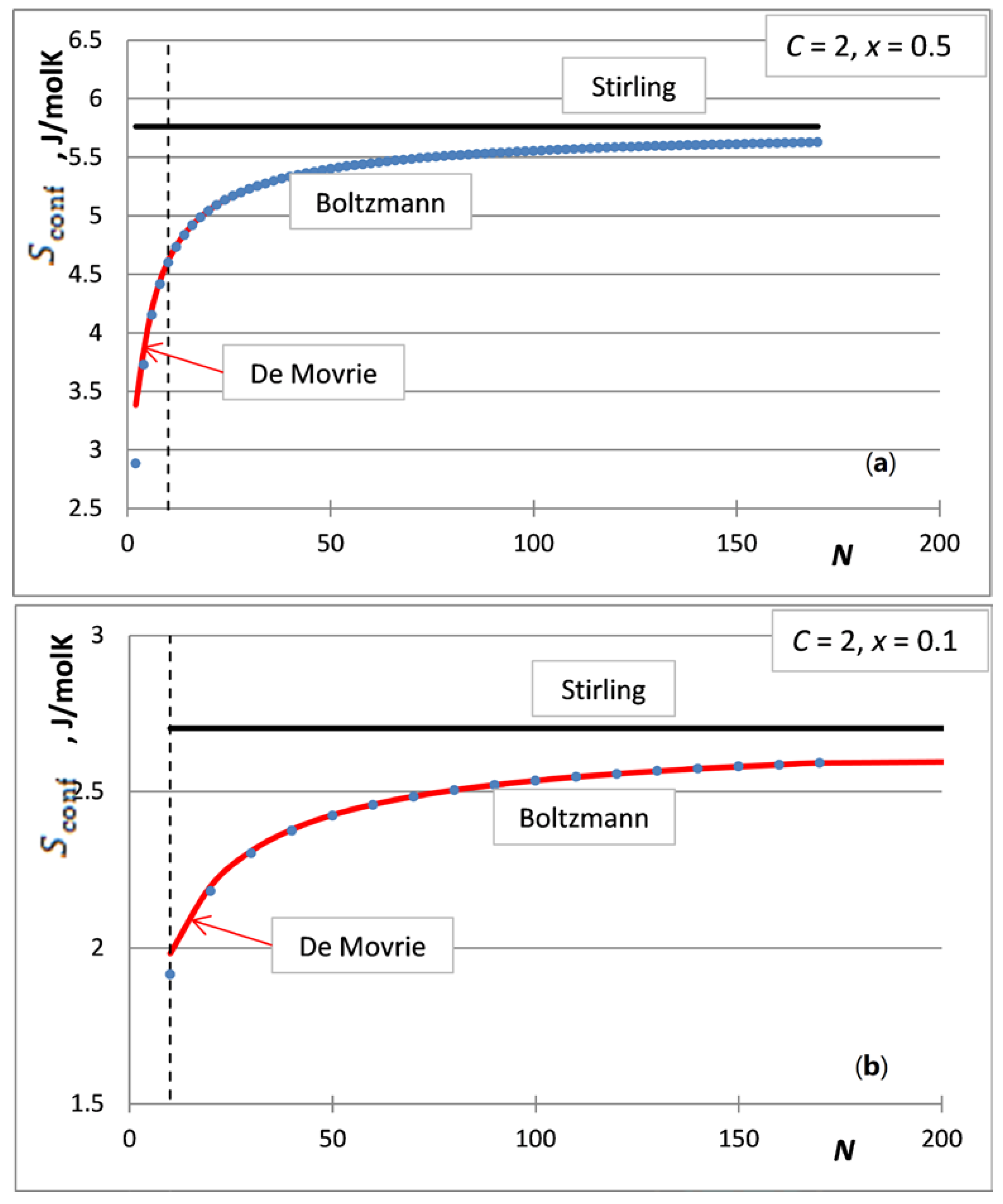
• The first case is the bulk calculations below the size of the solution phase, when the integral entropies calculated by the Stirling approximation lead to more than 0.1% relative error compared to the de Moivre approximation (in this case, this error cannot be compared to the exact Boltzmann equation, as it cannot be calculated for large numbers). For example, the difference between the Stirling approximation and the de Moivre approximation becomes smaller than 0.1% for Figure 4a,b and Figure 5 at $N\ge 7000$, $N\ge 14,000$, and $N\ge 10,000$, respectively. Thus, the de Moivre approximation should be used whenever the number of atoms is below 15,000. Let us take the average molar volume of a metal (10 cm³/mol), leading to the volume of the phase 2.5 × 10⁻²⁵ m³. If it is a cubic phase, its side length equals 6.3 nm. For molecular solutions, this critical size will be larger, as the molecules are larger than the atoms.
• The second case is when surface or interface equilibrium calculations are performed, being routinely used in nano-equilibrium calculations. In this case, the de Moivre approximation should be used whenever the surface/interface region contains less than 15,000 atoms. Suppose a single layer of atoms along the surface and the average molar surface area of 45,000 m²/mol. Then, 15,000 atoms will cover a 1.2 × 10⁻¹⁵ m² surface area. If this phase is cubic, its side length is 13.7 nm. So, we can conclude that when the diameter of a nano-phase is below 15 nm, the de Moivre approximation should be used instead of the Stirling approximation. For molecular solutions, this critical size will be larger, as the molecules are larger than the atoms.

The last term of Equations (18)–(20) leads to incorrect values when they are used for solutions containing less than one atom per component. Thus, all the above equations should be used only at:

$$x_i<\frac{1}{N}$$

(22)

Equation (22) provides a reasonable limit, as there is no physical sense to conduct any calculation beyond it.

8. Conclusions

It is demonstrated that for nano-phases smaller than about 15 nm (in diameter), the Stirling approximation leads to a significant error in the molar entropy of solutions compared to its exact equation. This deviation increases with decreasing number of atoms/molecules in the phase, with increasing deviation of the composition of the solution from its equimolar value, and with increasing number of components in the phase. A new de Moivre approximation is suggested in this paper, which is able to correct the Stirling approximation as a function of the number of atoms/molecules in the solution and its composition for C-component solutions. The new de Moivre approximation is a continuous function of the number of atoms/molecules in the solution and its composition, and it can be easily calculated without running into the problem of too-large numbers, as is the case for the exact Boltzmann equation. The de Moivre approximation (as any other calculation) should be used only for cases when there is at least one atom of each component in the nano-solution.

References

1. Gibbs, J.W. On the Equilibrium of Heterogeneous Substances. Am. J. Sci. 1878, 96, 441–458. [Google Scholar] [CrossRef]
2. Thomson, W. On the Equilibrium of Vapour at a Curved Surface of Liquid. Proc. R. Soc. Edinb. 1872, 7, 63–68. [Google Scholar] [CrossRef]
3. Ostwald, W. Über die vermeintliche Isomerie des roten und gelben Quecksilberoxyds und die Oberflächenspannung fester Körper. Z. Phys. Chem. 1900, 34, 495–503. (In German) [Google Scholar] [CrossRef]
4. Pawlow, P. Über die Abhängigkeit des Schmelzpunktes von der Oberflächenenergie eines Festen Körpers. Z. Phys. Chem. 1908, 55, 545–548. (In German) [Google Scholar] [CrossRef]
5. Reiss, H.; Wilson, I.B. The Effect of Surface on Melting Point. J. Colloid Sci. 1948, 3, 551–561. [Google Scholar] [CrossRef]
6. Couchman, P.R.; Jesser, W.A. Thermodynamic theory of size dependence of melting temperature in metals. Nature 1977, 269, 481–483. [Google Scholar] [CrossRef]
7. Samsonov, V.M.; Malkov, O.A. Thermodynamic model of crystallization and melting of small particles. Cent. Eur. J. Phys. 2004, 2, 90–103. [Google Scholar] [CrossRef]
8. Lee, J.H.; Tanaka, T.; Lee, J.; Mori, H. Effect of substrates on the melting temperature of gold nanoparticles. Calphad 2007, 31, 105–111. [Google Scholar] [CrossRef]
9. Kaptay, G. On the size and shape dependence of the solubility of nano-particles in solutions. Int. J. Pharm. 2012, 430, 253–257. [Google Scholar] [CrossRef] [PubMed]
10. Junkaew, A.; Ham, B.; Zhang, X.; Arróyave, R. Tailoring the formation of metastable Mg through interfacial engineering: A phase stability analysis. Calphad 2014, 45, 145–150. [Google Scholar] [CrossRef]
11. Guenther, G.; Guillon, O. Models of size-dependent nanoparticle melting tested on gold. J. Mater. Sci. 2014, 49, 7915–7932. [Google Scholar] [CrossRef]
12. Kaptay, G.; Janczak-Rusch, J.; Pigozzi, G.; Jeurgens, L.P.H. Theoretical Analysis of Melting Point Depression of Pure Metals in Different Initial Configurations. J. Mater. Eng. Perform. 2014, 23, 1600–1607. [Google Scholar] [CrossRef]
13. Zhu, J.; Fu, Q.; Xue, Y.; Cui, Z. Comparison of different models of melting transformation. J. Mater. Sci. 2016, 51, 2262–2269. [Google Scholar] [CrossRef]
14. Arabczyk, W.; Ekiert, E.A.; Pelka, R. Hysteresis phenomenon in a reaction system of nanocrystalline iron and a mixture of ammonia and hydrogen. Phys. Chem. Chem. Phys. 2016, 18, 25796–25800. [Google Scholar] [CrossRef] [PubMed]
15. Kaptay, G.; Janczak-Rusch, J.; Jeurgens, L.P.H.J. Melting Point Depression and Fast Diffusion in Nanostructured Brazing Fillers Confined between Barrier Nanolayers. Mater. Eng. Perform. 2016, 25, 3275–3284. [Google Scholar] [CrossRef]
16. Weismuller, J. Alloy Effects in Nanostructures. Nanostruct. Mater. 1993, 3, 261–272. [Google Scholar] [CrossRef]
17. Badmos, A.Y.; Bhadeshia, H.K. The Evolution of Solutions: A Thermodynamic Analysis of Mechanical Alloying. Metall. Mater. Trans. 1997, 28A, 2189–2194. [Google Scholar] [CrossRef]
18. Jesser, W.A.; Shiflet, G.J.; Allen, G.L.; Crawford, J.L. Equilibrium phase diagrams of isolated nano-phases. Mater. Res. Innov. 1999, 2, 211–216. [Google Scholar] [CrossRef]
19. Wautelet, M.; Dauchot, J.P.; Hecq, M. Phase diagrams of small particles of binary systems: A theoretical approach. Nanotechnology 2000, 11, 6–9. [Google Scholar] [CrossRef]
20. Tanaka, T.; Hara, S. Thermodynamic Evaluation of Binary Phase Diagrams of Small Particle Systems. Z. Metall. 2001, 92, 467–472. [Google Scholar]
21. Lee, J.G.; Mori, H. In-situ observation of alloy phase formation in nanometre-sized particles in the Sn–Bi system. Rechtsphilos. Mag. 2004, 84, 2675–2686. [Google Scholar] [CrossRef]
22. Shirinayan, A.S.; Gusak, A.M. Phase diagrams of decomposing nanoalloys. Rechtsphilos. Mag. 2004, 84, 579–593. [Google Scholar] [CrossRef]
23. Lee, J.; Lee, J.; Tanaka, T.; Mori, H.; Penttilá, K. Phase Diagrams of Nanometer-Sized Particles in Binary Systems. JOM 2005, 57, 56–59. [Google Scholar] [CrossRef]
24. Qiao, Z.; Cao, Z.; Tanaka, T. Prediction of surface and interfacial tension based on thermodynamic data and CALPHAD approach. Rare Met. 2006, 25, 512–528. [Google Scholar] [CrossRef]
25. Braidy, N.; Purdy, G.R.; Botton, G.A. Equilibrium and stability of phase-separating Au–Pt nanoparticles. Acta Mater. 2008, 56, 5972–5983. [Google Scholar] [CrossRef]
26. Lee, J.; Park, J.; Tanaka, T. Effects of interaction parameters and melting points of pure metals on the phase diagrams of the binary alloy nanoparticle systems: A classical approach based on the regular solution model. Calphad 2009, 33, 377–381. [Google Scholar] [CrossRef]
27. Eichhammer, Y.; Heyns, M.; Moelans, N. Calculation of phase equilibria for an alloy nanoparticle in contact with a solid nanowire. Calphad 2011, 35, 173–182. [Google Scholar] [CrossRef]
28. Kaptay, G. Nano-Calphad: Extension of the Calphad method to systems with nano-phases and complexions. J. Mater. Sci. 2012, 47, 8320–8335. [Google Scholar] [CrossRef]
29. Garzel, G.; Janczak-Rusch, J.; Zabdyr, L. Reassessment of the Ag–Cu phase diagram for nanosystems including particle size and shape effect. Calphad 2012, 36, 52–56. [Google Scholar] [CrossRef]
30. Lee, J.; Sim, K.J. General equations of CALPHAD-type thermodynamic description for metallic nanoparticle systems. Calphad 2014, 44, 129–132. [Google Scholar] [CrossRef]
31. Ghasemi, M.; Zanolli, Z.; Stankovski, M.; Johansson, J. Size- and shape-dependent phase diagram of In–Sb nano-alloys. Nanoscale 2015, 7, 17387. [Google Scholar] [CrossRef] [PubMed]
32. Bajaj, S.; Haverty, M.G.; Arróyave, R.; Goddard, W.A., III.; Shankar, S. Phase stability in nanoscale material systems: extension from bulk phase diagrams. [CrossRef] [PubMed]
33. Pelegrina, J.L.; Gennari, F.C.; Condó, A.M.; Guillemet, A.F. Predictive Gibbs-energy approach to crystalline/amorphous relative stability of nanoparticles: Size-effect calculations and experimental test. J. Alloys Compd. 2016, 689, 161–168. [Google Scholar] [CrossRef]
34. Leitner, J.; Sedmidubskỳ, D. Enhanced solubility of nanostructured paracetamol. Biomed. Phys. Eng. Express 2016, 2, 0555007. [Google Scholar] [CrossRef]
35. Shardt, N.; Elliott, J.A.W. Thermodynamic Study of the Role of Interface Curvature on Multicomponent Vapor−Liquid Phase Equilibrium. J. Phys. Chem. A 2016, 120, 120–2194. [Google Scholar] [CrossRef] [PubMed]
36. Lewis, G.N.; Randall, M. Thermodynamics; McGraw-Hill Book Co.: New York, NY, USA, 1923. [Google Scholar]
37. Lupis, C.H.P. Chemical Thermodynamics of Materials; Elsevier: Amsterdam, The Netherland, 1983. [Google Scholar]
38. Atkins, P.; de Paula, J. Physical Chemistry; Oxford University Press: Oxford, UK, 2002. [Google Scholar]
39. Lukas, H.L.; Fries, S.G.; Sundman, B. Computational Thermodynamics: The Calphad Method; Cambridge University Press: Cambridge, UK, 2007. [Google Scholar]
40. Saunders, N.; Miodownik, A.P. CALPHAD (Calculation of Phase Diagrams): A Comprehensive Guide; Elsevier: Amsterdam, The Netherlands, 1998; p. 479. [Google Scholar]
41. Stirling, J. Methodus Differentialis; Ap. Whiston & White: London, UK, 1764. (In Latin) [Google Scholar]
42. Tweddle, I. James Stirling’s Methodus Differentialis: An Annotated Translation of Stirling’s Text; Springer: Berlin/Heidelberg, Germany, 2012. [Google Scholar]
43. Boltzmann, L. Über die beziehung dem zweiten Haubtsatze der mechanischen Wärmetheorie und der Wahrscheinlichkeitsrechnung respektive den Sätzen über das Wärmegleichgewicht. Wien. Ber. 1877, 76, 373–435. (In German) [Google Scholar]
44. Sharp, K.; Matschinsky, F. Translation of Ludwig Boltzmann’s Paper “On the Relationship between the Second Fundamental Theorem of the Mechanical Theory of Heat and Probability Calculations Regarding the Conditions for Thermal Equilibrium” Sitzungberichte der Kaiserlichen Akademie der Wissenschaften. Mathematisch-Naturwissen Classe. Abt. II, LXXVI 1877, pp. 373–435 (Wien. Ber. 1877, 76:373–435). Reprinted in Wiss. Abhandlungen, Vol. II, reprint 42, pp. 164–223, Barth, Leipzig, 1909. Entropy 2015, 17, 1971–2009. [Google Scholar] [CrossRef]
45. Leubner, C. Generalised Stirling approximations to N! Eur. J. Phys. 1985, 6, 299–301. [Google Scholar] [CrossRef]
46. Nemes, G. New asymptotic expansion for the Gamma function. Arch. Math. 2010, 95, 161–169. [Google Scholar] [CrossRef]
47. Mortici, C. Ramanujan formula for the generalized Stirling approximation. Appl. Math. Comput. 2010, 217, 699–704. [Google Scholar] [CrossRef]
48. Lin, L. On Stirling’s formula remainder. Appl. Math. Comput. 2014, 247, 494–500. [Google Scholar] [CrossRef]
49. Mortici, C. A new fast asymptotic series for the gamma function. Raman. J. 2015, 38, 549–559. [Google Scholar] [CrossRef]
50. Lu, D.; Song, L.; Ma, C. Some new asymptotic approximations of the gamma function based on Nemes’ formula, Ramanujan’s formula and Burnside’s formula. Appl. Math. Comput. 2015, 253, 1–7. [Google Scholar] [CrossRef]
51. Xu, A.; Hu, Y.; Tang, P. Asymptotic expansions for the gamma function. J. Number Theory 2016, 169, 134–143. [Google Scholar] [CrossRef]
52. Chen, C.P. On the asymptotic expansions of the gamma function related to the Nemes, Gosper and Burnside formulas. Appl. Math. Comput. 2016, 276, 417–431. [Google Scholar] [CrossRef]
Figure 1. The dependence of the integral molar configurational entropy of a binary, equimolar solution on the number of atoms/molecules in it, calculated by Equation (1) called the “Stirling approximation” and Equation (6) called the “exact Boltzmann equation” (C = the number of components).
Entropy 19 00248 g001
Figure 2. The relative error in integral molar configurational entropy values of binary solutions as function of the number of atoms/molecules calculated by Equation (9) (numbers on the curves are the mole fractions of any of the component in the solution).
Entropy 19 00248 g002
Figure 3. The relative error in integral molar configurational entropy values of equimolar solutions as function of the number of atoms/molecules calculated by Equation (9) (numbers on the curves equal the number of components in the solution).
Entropy 19 00248 g003
Figure 4. The dependence of the integral molar configurational entropy of a binary solution on the number of atoms/molecules in it, calculated by Equation (1) called the “Stirling approximation” (horizontal bold line), Equation (6) called the “exact Boltzmann equation” (points), and by Equation (13) called the “de Moivre approximation” (line mostly across the points). The vertical dotted line corresponds to N = 10. (a) Corresponds to the equimolar solution, while the bottom figure (b) corresponds to the solution with 0.1 or 0.9 mole fractions of the components.
Entropy 19 00248 g004
Figure 5. The dependence of the integral molar configurational entropy of the equimolar five-component solution on the number of atoms/molecules in it, calculated by Equation (1) called the “Stirling approximation” (horizontal bold line), Equation (7) called the “exact Boltzmann equation” (points), and by Equation (13) called the “de Moivre approximation” (line mostly across the points). The vertical dotted line corresponds to N = 10.
Entropy 19 00248 g005