1. Introduction
Complex networks are used as a medium for transmitting contents within online social platforms and other computer systems. Information spreading processes are a basement of viral marketing [
1], rumours [
2], social and political changes [
3], innovation adoption [
4] and other initiatives with emotional appeal [
5]. Possible types of contents propagated within electronic systems include texts [
6], concepts [
7], video material [
8], images [
9] and marketing messages [
10]. Research in this area is, among others, related to information flow within the networks [
11], factors affecting performance of marketing campaigns [
12] and the selection of highly influential nodes [
13]. Campaigns based on information spreading can be targeted to increase the number of customers reached within the network [
14], or alternatively can have quite the opposite goal, namely, to decrease disease transmission [
15]. Models from epidemic research, such as SIR (Susceptible-Infected-Recovered) or SIS (Susceptible-Infected-Susceptible) [
16], were implemented for the purposes of analyzing the spread of information with their extensions targeted to indirect and direct transmission [
17] or heterogeneous networks [
18]. Other approaches are based on an independent cascades model [
14], linear threshold model [
19] or branching processes [
20]. Recent works have focused on spreading processes in multilayer [
21] and temporal networks [
22], with the representation closer to reality than the static networks.
Intentional initialisation of information spreading processes is usually based on the selection of starting nodes to launch information cascades within the network. Node selection and activation, known as a seeding process [
23], are focused on selection of highly influential nodes [
24] and can be based on a number of approaches including selection of candidates with the highest degree of other network centrality measures with assumed high potential for information spreading [
23]. More complicated solutions with high computational costs are based on greedy approach and its extensions towards optimal seed set selection [
14] or data mining techniques [
25]. The majority of earlier studies assumed single stage seeding as well as selection of seeds at the beginning of the process. After seed selection, information spreading continues through the use of natural mechanisms without additional support. Preliminary works are associated with adaptive solutions, using the knowledge gathered during the process in order to improve overall performance [
26]. Other approaches take into account multiple ongoing campaigns and relations between them [
27].
Recent studies optimised the usage of structural measures to refrain from selecting nodes in the same segments of network for better allocation of seeds. Solutions of this type are based on sequential seeding for better usage of natural diffusion processes [
28], targeting communities to avoid seeding of nodes within the same communities with close intra connections [
29] and a usage of voting mechanisms with decreased weights after detection of already activated nodes [
30]. In other studies, a k-shell based approach was implemented in order to detect central nodes within the networks [
31].
Our earlier research showed that the seeding process in the form of a sequence delivers better results than using the same number of seeds at the beginning of the process [
28]. The main reason of enhanced performance is the fact that some of the nodes activated as seeds in single stage seeding have a potential to be activated as a result of natural diffusion. The budget allocated to seeding can be used for activating other nodes. It leads to better usage of the resources and results in better outcomes in terms of coverage represented by a percentage of activated nodes within the network.
For seed selection in the sequential seeding in all stages of the process, the centrality measures computed at the beginning of the process were used. In the current research, we assumed that the performance of sequential seeding could be further improved with the dynamic rankings to better address topological dynamics problem [
32]. The recalculation of network measures used for seed selection in each seeding stage was performed and the effective degree and second level degree computed using inactivated nodes only was introduced. Results showed that recalculation of centrality measures in each stage delivers better results, albeit leading to higher usage of computational resources. Selection of the final solutions is based on the trade-off between coverage and the use of computational resources.
The paper is organised as follows. In
Section 2, the proposed approach is presented with an illustrative example. Experiment design and results are presented in
Section 3. In
Section 4, the search for trade-off between coverage and computational cost is discussed and followed by conclusions in
Section 5.
2. Materials and Methods
The approach presented in this paper is based on the sequential seeding that is performed in continuation during the whole process, but not in single stage as in most of the earlier methods [
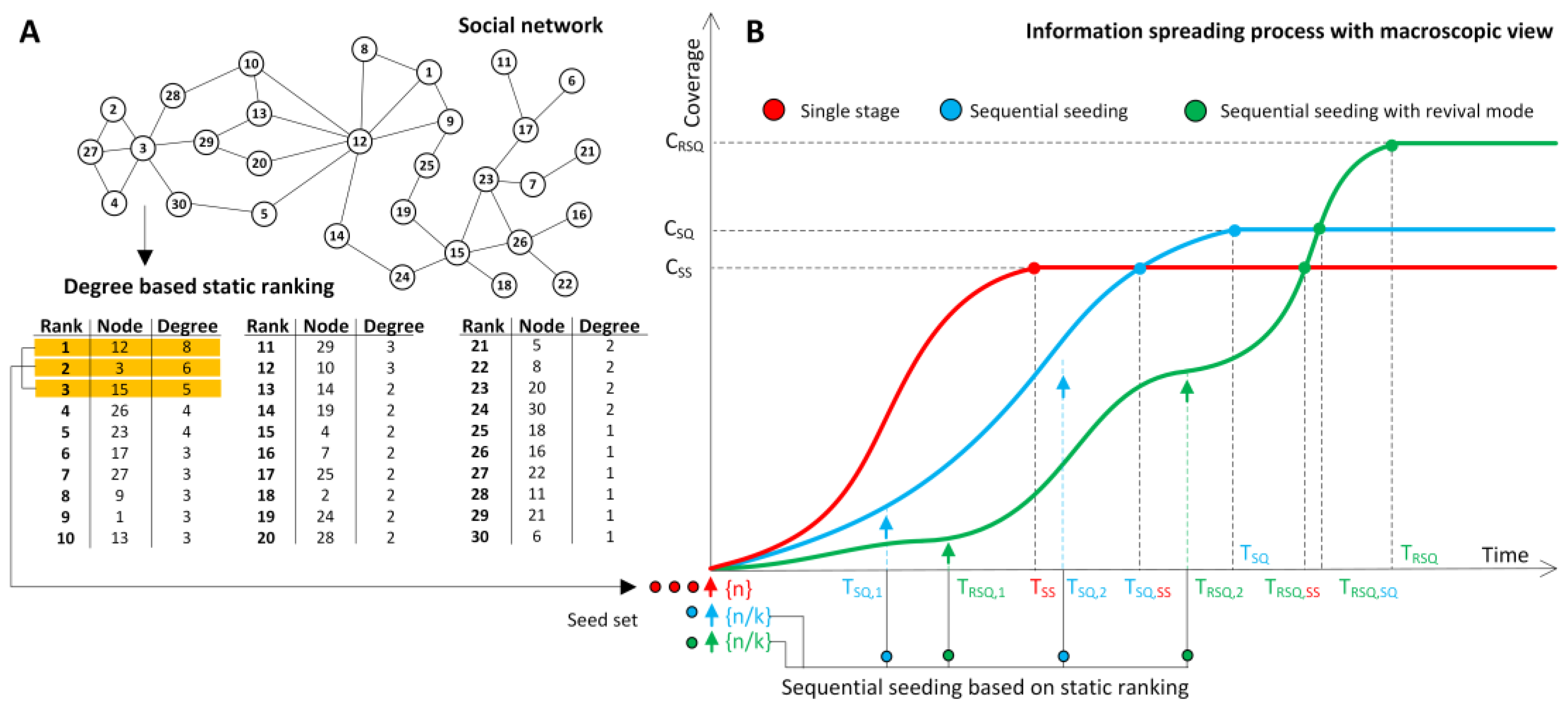
28]. The main concept of sequential seeding is based on a sequence of seeds instead of using all in a single step to deliver a better result due to the potential of a natural diffusion process. If all seeds are used in a single step, some seeds are wasted for activation of nodes with the potential to be infected naturally. In sequential seeding, saved seeds are used to infect more difficult to reach nodes. Consequently, the number of activated nodes increases. Seeds are selected using ranking based on one of the centrality measures such as the degree created before the process is initiated, as is illustrated in
Figure 1A. In single stage seeding (SS), all top
n seeds from the ranking would be used to initiate diffusion process illustrated by a red line in
Figure 1B. The information process continues without any additional support until it reaches coverage C
SS in time T
SS. Sequential seeding SQ is performed in
k stages and, in each stage,
n/
k seeds are selected and used. For seed selection, the same ranking computed at the beginning the process is still used. Two types of sequential seeding are considered. The blue line in
Figure 1B illustrates an example generic sequential seeding process with two seeding stages where additional seeding takes in a priori assigned time points (e.g., in subsequent simulation stages) denoted as T
SQ,1 and T
SQ,2, no matter if the natural process continues or not. Another form of sequential seeding, illustrated by the green line in
Figure 1B, is based on the revival mode and additional seeding takes place when the process dies out in detected time points T
RQS,1 and T
RSQ,2 when natural diffusion is not continued. Time points, when processes based on sequential seeding and sequential seeding with revival mode terminates, are denoted by T
SQ and T
RSQ, respectively.
Results from our earlier research showed that coverage CSQ is greater than CSS for most simulation cases, owing to better usage of natural diffusion potential. In contrast, the process based on the sequential seeding lasts longer, and, at the time TSQ,SS when the process based on the sequential seeding SQ reaches the single stage SS coverage, CSS is greater than TSS. Revival mode improves the coverage and CRSQ > CSQ for most cases, but, at the time when at least the coverage from a single stage approach is reached, TRSQ,SS > TSQ,SS. However, in the example, the degree based strategy was used, and the static rankings approach for sequential seeding can be applied to all node selection strategies related to centrality measures. Sequential seeding with the revival mode based on static rankings is illustrated with Algorithm 1.
| Algorithm 1: Sequential Seeding with Static Ranking and Revival Mode |
| Input: Graph G(V,E), PropagationProbability, SeedingPercentage |
| Output: set of activated nodes ActiveNodes, initially ActiveNodes = {} |
| 0: Initialize: stage s = 0; NumberOfSeeds = SeedingPercentage * NumberOfNodes(G); k = number of seeds in the stage |
| 1: for each node v є V |
| 2: Compute network measure m(v) |
| 3: end for |
| 4: Create initial ranking R of nodes sorted by measure m(v) in the descending order |
| 5: SeedSet = top k nodes from ranking R /* seeds for stage s = 0 */ |
| 6: while NumberOfSeeds > 0 |
| 7: Activate each node from SeedSet |
| 8: ActiveNodes = ActiveNodes ∪ SeedSet |
| 9: R = R\SeedSet /* remove recent seeds from the ranking to avoid double seeding */ |
| 10: NumberOfSeeds = NumberOfSeeds − |SeedSet| /* note that in the last stage |SeedSet| may be < k */ |
| 11: ActivatingNodes = SeedSet |
| 12: % information diffusion process according to IC model starts here |
| 13: while |ActivatingNodes| > 0 |
| 14: for each node i from ActivatingNodes |
| 15: for each not yet activated neighbor j of node i in G(E,V) |
| 16: Generate random number Rand from the range <0,1> |
| 17: if Rand <= PropagationProbability |
| 18: Activate node j |
| 19: ActiveNodes = ActiveNodes ∪ {j} |
| 20: ActivatingNodes = ActivatingNodes ∪ {j} /* neighbor j of k is active and may activate others */ |
| 21: R = R\{j} /* remove activated nodes from the ranking—the crucial part of the sequential algorithm*/ |
| 22: end if |
| 23: end for |
| 24: ActivatingNodes = ActivatingNodes\{i} /* remove i from activating nodes */ |
| 25: end for |
| 26: end while |
| 27: % information diffusion process dies out |
| 28: if NumberOfSeeds > 0 |
| 29: % preparation for revival and selection of new seed candidates |
| 30: SeedSet = top min(k,NumberOfSeeds) nodes from ranking R /* seed set for the next stage s + 1 */ |
| 31: s = s + 1 |
| 32: end if |
| 33: end while |
Network measures computed only once may lead to a situation when a good candidate for influential seeds with a high position in the ranking at the beginning when selected as a seed no longer has a high potential, as the majority of neighbours were infected earlier. At the beginning stages of the process, it may be less important, but if the diffusion process continues for a longer time, it may result in a not fully used potential of seeds. To overcome such problems, an approach based on effective network measures and dynamic ranking created in each stage based on network measures computed with the use of non-infected nodes only is presented is illustrated with Algorithm 2.
| Algorithm 2: Sequential Seeding with Dynamic Ranking and Revival Mode |
| Input: Graph G(V, E), PropagationProbability, SeedingPercentage |
| Output: set of activated nodes ActiveNodes, initially ActiveNodes = {} |
| 0: Initialize: stage s = 0; NumberOfSeeds = SeedingPercentage * NumberOfNodes(G); UsedSeeds = 0; k = number of seeds in the stage |
| 1: for each node v є V |
| 2: Compute network measure m(v) |
| 3: end for |
| 4: Create initial ranking R0 of nodes sorted by measure m(v) in the descending order |
| 5: SeedSet0 = top k nodes from ranking R0 /* seeds for stage s = 0 */ |
| 6: while NumberOfSeeds > 0 |
| 7: Activate each node from SeedSets |
| 8: ActiveNodes = ActiveNodes ∪ SeedSets |
| 9: NumberOfSeeds = NumberOfSeeds − |SeedSets| /* note that in the last stage |SeedSets| may be < k */ |
| 10: ActivatingNodes = SeedSets |
| 11: % information diffusion process according to IC model starts here |
| 12: while |ActivatingNodes| > 0 |
| 13: for each node i from ActivatingNodes |
| 14: for each not yet activated neighbor j of node i in G(E,V) |
| 15: Generate random number Rand from the range <0,1> |
| 16: if Rand <= PropagationProbability |
| 17: Activate node j |
| 18: ActiveNodes = ActiveNodes ∪ {j}1 |
| 19: ActivatingNodes = ActivatingNodes ∪ {j} /* neighbor j of k is active and may activate others */ |
| 20: end if |
| 21: end for |
| 22: ActivatingNodes = ActivatingNodes\{i} /* remove i from activating nodes */ |
| 23: end for |
| 24: end while |
| 25: % information diffusion process dies out |
| 26: if NumberOfSeeds > 0 |
| 27: % preparation for revival and ranking recomputation |
| 28: for each not activated node v є V |
| 29: Compute network measure m(v) with the use of use of not activated nodes only |
| 30: end for |
| 31: Create updated ranking Rs+1 for next stage s + 1 of nodes sorted by measure m(v) in the descending order |
| 32: SeedSets+1 = top k nodes from ranking Rs+1 |
| 33: s = s + 1 |
| 34: end if |
| 35: end while |
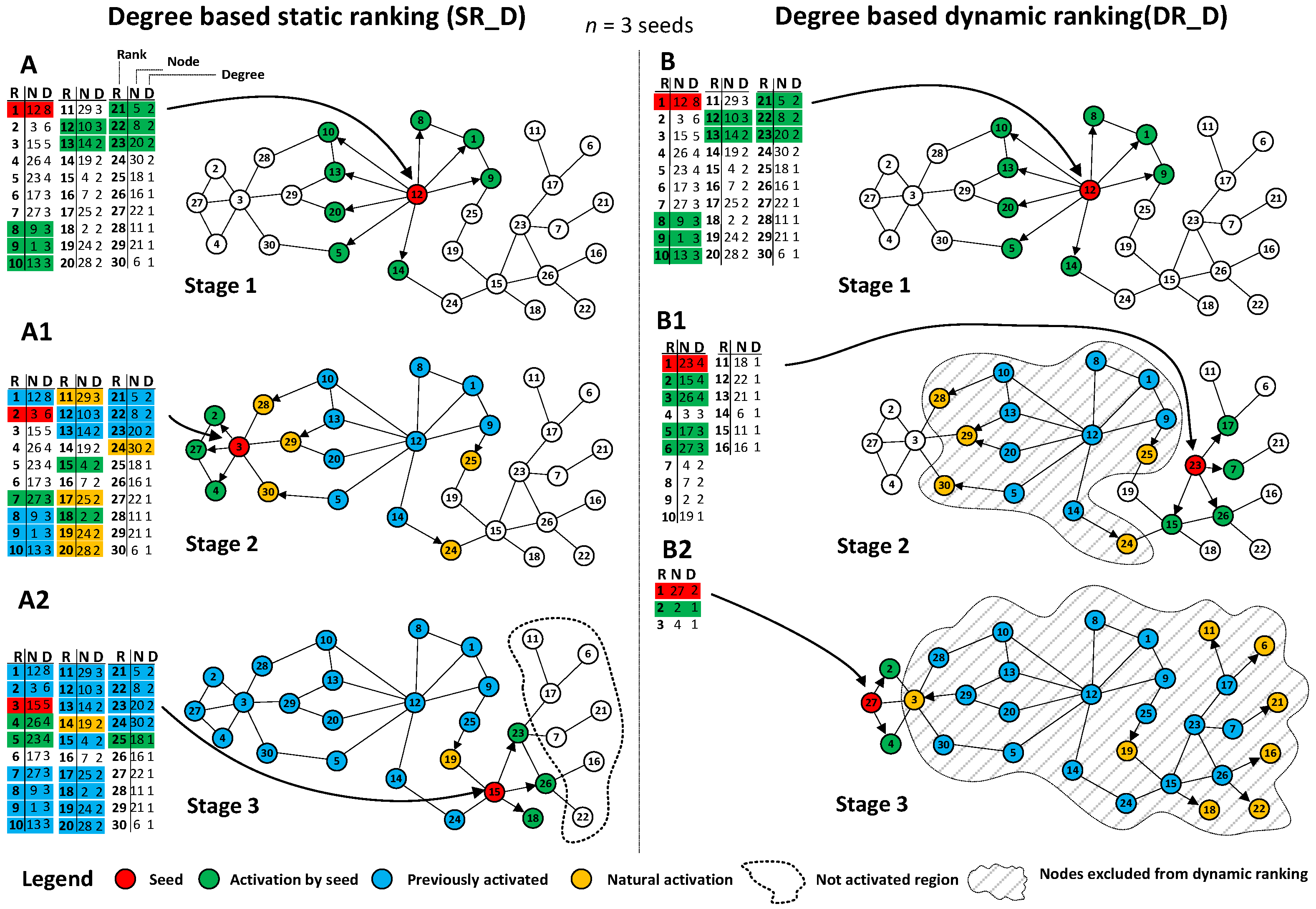
Figure 2A with a detailed description in the caption provides a microscopic example of a three stage process based on sequential seeding with one seed used in each stage and static ranking SR_D computed once and used at all stages. After three stages, seven nodes are left inactivated.
Figure 2B illustrates a process on the same network with three stages and three seeds used but with dynamic ranking DR_D computed with the use of an effective degree in each stage. The process resulted in improved coverage and all nodes were activated, owing to the usage of effective degree based on inactivated neighbours only.
The presented approach was illustrated using degree for simplicity; however, it can be applied to any other centrality measure with taken inactivated nodes only instead of using all nodes within network. Recalculations can be done for a second level degree with the use of the number of neighbours and the total number of their neighbours, closeness, betweenness, clustering coefficient or Page Rank. Further research concentrated on degree, second level degree and compared results from static and dynamic rankings with the use of agent based simulations. The approach presented in this paper is based on several extensions when compared to generic sequential seeding. The concept of dynamic rankings being recomputed before the revival takes place is a form of a new meta method, which can be widely used for improving information spreading processes. Effective network measures based on neighboring nodes with specific state only (not activated in our case) are introduced and other centrality measures can use a similar approach. Research assumes a compromise between the usage of computational resources and the increase of coverage within the network, which shows a new perspective for analysis of information spreading processes. The presented results indicate how intervals between recomputations are affecting coverage.
3. Results
Experiments were designed and performed using the agent-based simulations on 15 static real networks N1–N15, containing from 899 to 16,264 nodes with characteristics and references presented in
Table 1 and references to related papers. Average values of main network parameters for each used network are presented including degree (D), second level degree (D2), closeness (CL), PageRank (PR), eigenvector (EV) and clustering coefficient (CC).
The independent cascades model (IC) was used for simulations and even single seed can induce information cascades, while, for example, in a linear threshold model (LT), a small seed set would have no effect [
14]. With propagation probability PP (
a,
b), node
a activates (influences or infects) node
b in the step
t + 1 under the condition that node
a was activated at time
t. Parameters used in simulations characterising information propagation, networks, and strategies for seed selection are presented in
Table 2.
Simulation parameters create an experimental space N × R × PP × SP × S resulting into 6750 configurations. For each configuration, results from 100 simulation runs were averaged. Sequential seeding based on single seed per stage with revival mode (RSQ) was used owing to its superior performance when compared to non-revival mode (SQ). The agent based model was implemented, with agents connected according to the networks specifications. Each step of simulation includes the selection of additional seeds (if additional seeding is allowed), contacting all nodes activated in the previous step and newly selected seeds and finally activating their neighbours according to the propagation probability. The simulation results achieved with no-recalculation approach R0 based on not recomputed degree D and not recomputed second level degree D2 were compared with approach based on recalculations of corresponding network metrics with various frequencies Rk, where k denotes the number of simulation steps between recalculations with used values R1, R2, R4, R6, R16, R32, R64, R128 and R256. Comparisons were performed using the same network (N) with the same parameters including sequential strategy with revival mode (RSQ), propagation probability (PP), seeding percentage (SP) and seed selection strategy (S) based on recalculated degree (D) and second level degree (D2), respectively.
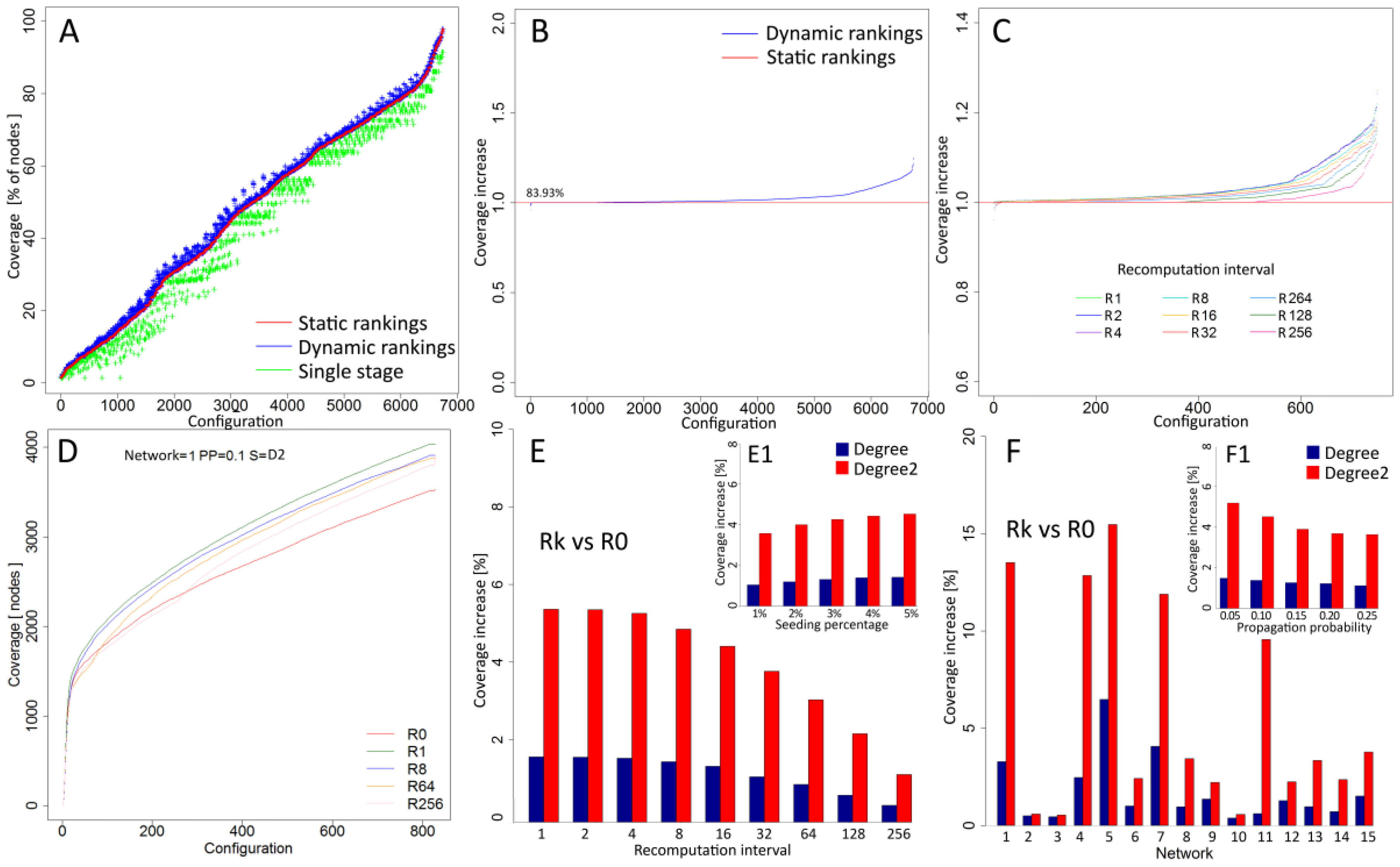
Coverage of information spreading processes initiated by seeds selected from dynamic rankings was compared with static rankings and averaged results for all simulation configurations N × R × PP × SP × S are shown in
Figure 3A. An average increase of 2.73% for all cases in relation to results based on the not recomputed network measures denoted by red line was observed. For comparison, results from single stage approach with lower coverage for most cases are presented in green. Wilcoxon test for dynamic ranking vs. static ranking shows statistical significance (
p-value < 2.2 × 10
−16) and Hodges–Lehmann estimator Δ = 0.74 confirms higher performance of proposed approach. In 83.93% of cases, recalculation delivered better coverage than approaches without recalculation (
Figure 3B).
Figure 3C shows increase for each recalculation interval R1, R2, R4, R8, R16, R32, R64, R128 and R256. Recalculations performed in every step denoted as R1 delivered better performance in 99.87% cases while the longest interval R256 with interval equal to 256 steps delivered improvement in 33.2% of cases. For example, detailed results from simulations based on second level degree D2, static (red line) and dynamic approaches with various recalculation intervals (R1, R8, R64, R256) within network N1 with propagation probability PP = 0.1 and seeding percentage SP = 5% are showed in
Figure 3D. Coverage increase was dependent on recalculation frequency with the highest average increase of 3.69% for R1 (
p-value < 2.2 × 10
−16, Δ = 0.84) and dropping through other intervals to 0.86% achieved for R256 (
p-value < 2.2 × 10
−16, Δ = 0.54). Dynamic rankings were more effective for second level degree (D2) than for degree (D).
Figure 3E reveals a 5.64% increase for D2 (
p-value < 2.2 × 10
−16, Δ = 1.34) for R1 interval and a 1.73% increase for DD with the same interval (
p-value < 2.2 × 10
−16, Δ = 0.49).
In terms of seeding percentage (SP), the number of seeds affected performance with overall results is shown in
Figure 3E1. For degree, the lowest performance increase (1.06%) was observed for 1% seeding percentage, while, for SP = 5%, the performance improvement was 1.36 times higher (1.44%). A similar difference in results between smallest and highest seeding percentage was observed for second level degree with values 3.58% and 4.53%, respectively, and 1.27 times higher coverage for SP = 5% than for 1%. Performance of the approach based on recalculations is dependent on the parameters of information spreading process. The highest increase of dynamic rankings with recalculations was observed for lowest propagation probability PP = 0.05, whereas the lowest increase was observed for the propagation probability PP = 0.25 (
Figure 3F1). Bigger differences were observed for a second level degree (D2) than for degree (D). Performance of recalculations for PP = 0.05 was 1.43 times higher for D2 and 1.32 times higher for D when compared to PP = 0.25.
Apart from process characteristics, results were analysed for each network separately. Charts in
Figure 3F for recalculation interval R1 show varying results among networks. For all networks, a higher increase of performance was observed for second level degree (D2) than for degree (D). The largest difference was observed for network N1 with performance for D2 (9.56%), which was 15.67 times higher than for D (0.61%). The lowest difference was observed for network N2 with performance of D2 (0.58%), which was 1.18 times higher than D performance (0.49%). Networks N2, N3, and N10 with the lowest performance have a relatively high average degree with values 21.38, 31.19 and 74.85, respectively (see
Table 1). With larger degree information, spreads with high dynamics and greater coverage are reached regardless of strategy employed. Networks with high performance of dynamic rankings like N1, N4, N5, N7, and N11 are characterised by much lower average degrees such as 5.85, 2.67, 3.75 and 3.88, which results in lower coverage. In such conditions, recalculations of rankings improve results to a greater extent.
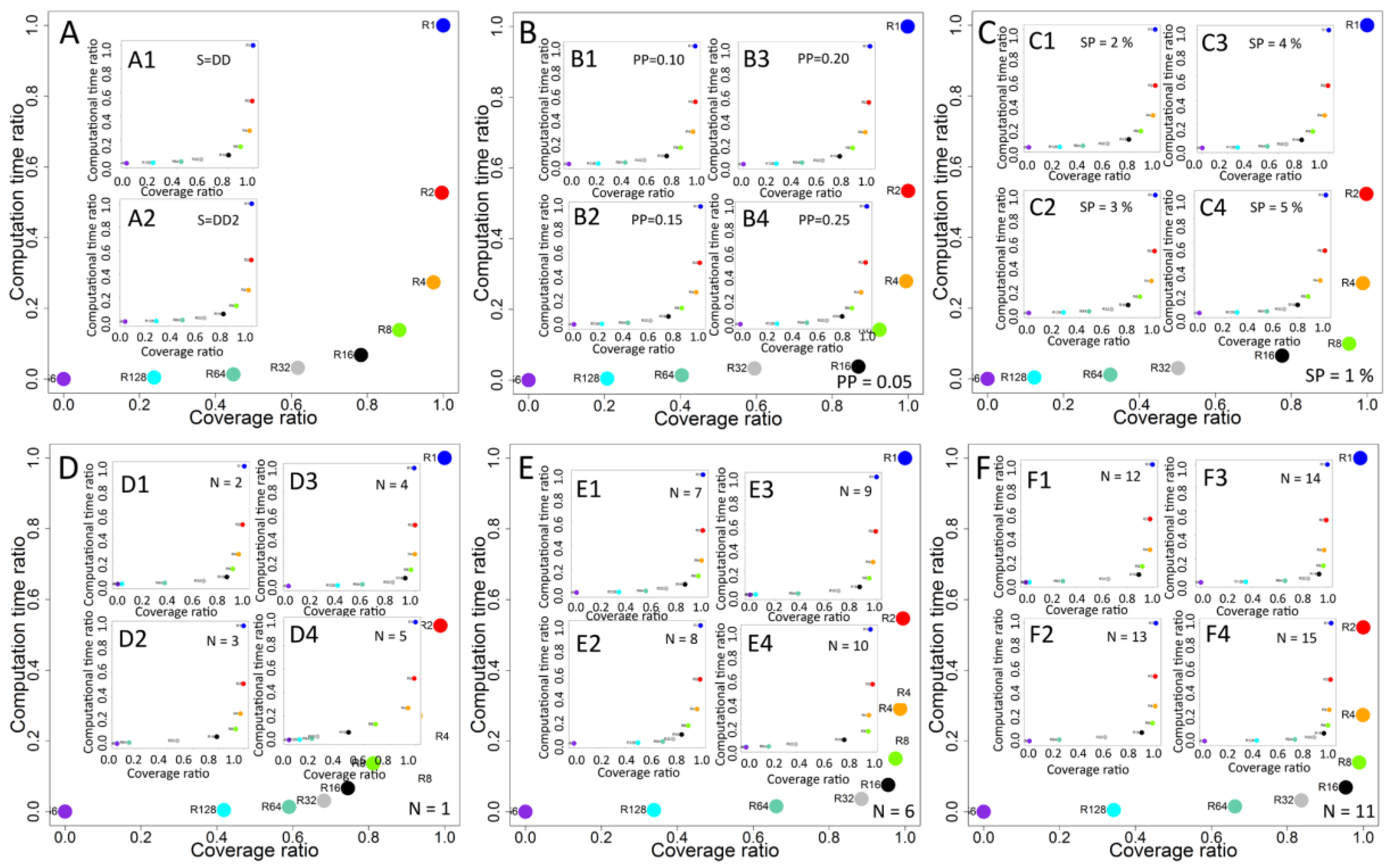
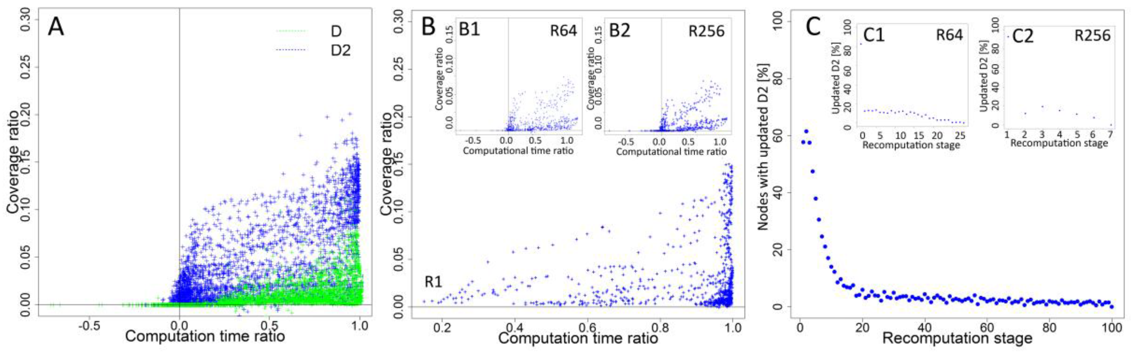
While recalculation increases the performance of information spreading process, the usage of computational resources and additional processing time affects the overall cost. Two-dimensional analysis was based on coverage ratio (C_R) and computation time ratio (CT_R). Coverage ratio was computed as a relation between coverage based on static and dynamic rankings according to the formula C_R = (C_DR–C_SR)/C_DR, where C_DR represents coverage of the process based on dynamic rankings seed selection and C_SR stands for coverage of static rankings approach for the same simulation configurations. Computational time ratio represents relationship between total time of computations of network measures during the process according to the formula C_TR = (T_DR–T_SR)/T_DR, where T_DR represents computational time for dynamic rankings and T_SR-computational time of static rankings for the same simulation configurations.
Figure 4A shows detailed results for each case and the relation between coverage and total computational time. An increase of coverage when dynamic rankings are used together with the increase of total computational time is observed. Comparison of results for degree (D) and second level degree (D2) shows higher increase of coverage for D2 even when time ratio reaches 0.5 of maximal values. For degree D, concentration of cases with best coverage is observed when the computational time ratio is closer to its maximal value.
In the next step, time and coverage ratios were computed for all cases for each recalculation frequency. Results for all experiment configurations and highest (R1), medium (R64) and lowest (R256) recalculation frequency are shown in
Figure 4B,B1,B2, respectively. Results for R1 (
Figure 4B) show increased coverage with more cases with higher values. Smaller concentration of cases close to maximal time ratio is observed for interval R64 (
Figure 4B1), while the highest concentration of low coverage cases is observed for R256 (
Figure 4B2). Results from simulations showed increased performance together with increased frequency of recalculations and updates of rankings before new seeds are selected. For recalculations, only inactivated nodes are taken into an account and their number is dropping as process continues. Analysis presented in
Figure 4C,C1,C2 for highest (R1), medium (R64) and lowest (R256) frequency of recalculations shows a decreasing number of affected nodes in each step of recalculation. For interval R256 (
Figure 4C2), results from all simulations show that, on average, recalculations were performed seven times for the diffusion process, and each recalculation affected, on average, 22.54% of nodes. For the R64 interval, the average number of updated nodes dropped to 10.42% (
Figure 4C1). For the smallest recalculation interval R1, the average number of updated nodes is equal to 6.31% (
Figure 4C).
4. Discussion
Final analysis presents the searching for trade-off solutions with potential to improve coverage with limited usage of computational resources. Normalised values of computational time ratio and normalised coverage ratio for each recalculation interval were used for better comparability of time and coverage between networks with different sizes and under different propagation parameters. The results obtained show the relationship between computational time and coverage for each recalculation interval for each experimental case (
Figure 5A).
Increasing frequency of recalculations and changing interval between recalculations from 256 to 128 steps resulted into growth of coverage ratio from 0 to 0.2384, while the computational time ratio increased from 0 to 0.0043. Results from R128 compared in relation to R64 show an increase of coverage ratio of 87.64% from 0.24 to 0.45 and a 211.08% increase of computational time ratio from 0.0043 to 0.0133. For further increase of recalculation frequency, the gains are smaller. R32 delivered results better by 26.95% in terms of coverage than R64, but the computational cost was increased by 114.13%. Further increase of the number of recalculations and shorter intervals for R16, R8 and R4 revealed a reduced increase of coverage ratio and an increase of computational time costs. Changing the interval from R32 to R16 increased the growth of coverage by 26.95% and by 114.13% of computational time, whereas an eight-step interval delivered 12.95% better coverage and 104.87% growth of computational time. Results show that, for frequent recalculations like R1, R2, R4, the differences in coverage are small, but computational time is increased significantly. When the interval was decreased from R8 to R4, a normalised coverage ratio for R4 achieved 0.9743 (10.14% increase when compared to R8) and computational time ratio achieved 0.2735 (97.32% increase when compared to R8). After increasing the frequency of recalculations to every two steps, the coverage ratio increased by 2.24% to 0.9961, while computational time ratio increased by 92.55% to the value of 0.5267. Recalculations performed in each step of simulation (R1) resulted into 89.87% increase of computational time ratio to 1.0, while a coverage ratio was increased only by 0.39% to 1.0 from 0.9961 obtained for R2. Similar relations are observed for analysis performed separately for degree D and second level degree D2 presented in
Figure 5A1,A2.
Differences in the coverage ratio for different recalculation intervals were dependent on propagation probability PP (
Figure 5B,B1–B4). Results for the lowest propagation probability PP = 0.05 (
Figure 5B) show lower differences between R1, R2 with 0.11% coverage increase and R2, R4 with 0.53% increase than observed for propagation probability PP = 0.25 (
Figure 5B4) and values obtained 1.03% for changing the interval from R2 to R1 and 3.67% after changing the interval from R4 to R2. Propagation probability PP = 0.25 resulted in a higher difference in coverage ratio after changing the interval from R256 to R128. Similar differences are observed for seeding percentage (
Figure 5C,C1–C4) between the lowest SP = 1% and the highest analysed SP = 5%. For SP = 1% (
Figure 5C), increasing the frequency of recalculations to R1 from a R2 interval resulted in 0.2% increase, while for SP = 5% (
Figure 5C4), the change is only 0.76%. Increasing frequency of recalculations from R4 to R2 resulted in an increased coverage ratio by 0.92% for SP = 1% and to 3.83% for SP = 5%.
Further analysis showed differences of obtained results dependent on network characteristics. Charts in
Figure 5D–F show the relationship between computational time ratio and coverage ratio for all analysed networks. For network N1, N4, N7, and N8, differences in coverage are observed between most of intervals with substantial difference between high intervals (R256, R128), medium intervals (R64, R32, R16) and the lowest intervals (R8, R4, R2, R1). For networks N2, N3, N5, N9, and N12, low differences between highest intervals are observed, while other differences are visible. Patterns observed for networks N6, N10, N11, N13, N14 and N15 show small differences for lowest intervals.
5. Conclusions
The presented research shows an extension to sequential seeding approach, initially based on seed selection with the use of static rankings. Results in terms of coverage were improved with the use of recalculation of network measures and the creation of new rankings during the process before additional seeding takes place. It makes possible better evaluation of the potential of seeding candidates when effective measures are used, while only taking into account inactivated nodes. It was verified with degree and second level degree where typical computation of degree takes into account all neighbours, while in the proposed solution, only not affected nodes are used in the form of effective degree for creating new rankings.
Overall, the results showed that seeds selection using effective measures improves coverage. Recalculation used with the second level degree increased the number of activated nodes at process end to a greater extent than for degree based selection. While recalculation of network measures in each seeding stage can result in an enhanced outcome, it also causes higher usage of computation resources for network measures updates. Recalculation in each stage of the process increases total recalculation time, while coverage is not much better than for intervals based on two or four stages between recalculation. Increased coverage was observed even for recalculations with longer intervals and lower cost represented by computation time ratio.
Analysis based on propagation parameters shows that recalculations are more effective for the process with lower propagation probability. In terms of characteristics of used networks, if the average degree is relatively large, the information spreading process has high dynamics, and high coverage is reached regardless of which strategy is used. Networks with high performance in dynamic rankings are characterised by much lower average degrees. Furthermore, in such conditions, the recalculation of rankings improves results.
Analysis of rankings and changes of network measures over the time shows that most nodes are affected at the beginning of the process. For better use of computational resources, more recalculations can be performed when higher dynamics of activation are observed and more nodes are activated. In such situations, recalculation results in larger changes in rankings and frequent calculations are justified.
The current research covered various parameters within experimental space; however, investigation can be extended in the future work. In the study, intervals between recalculation were permanent; however, they could be adapted to the dynamics of changes. Research used only degree and second level degree, and recalculation of other measures like closeness or betweenness could be performed. Apart from real datasets, artificial networks following theoretical network models can be used for more generalised results.


