Breakdown Point of Robust Support Vector Machines

Abstract

Support vector machine (SVM) is one of the most successful learning methods for solving classification problems. Despite its popularity, SVM has the serious drawback that it is sensitive to outliers in training samples. The penalty on misclassification is defined by a convex loss called the hinge loss, and the unboundedness of the convex loss causes the sensitivity to outliers. To deal with outliers, robust SVMs have been proposed by replacing the convex loss with a non-convex bounded loss called the ramp loss. In this paper, we study the breakdown point of robust SVMs. The breakdown point is a robustness measure that is the largest amount of contamination such that the estimated classifier still gives information about the non-contaminated data. The main contribution of this paper is to show an exact evaluation of the breakdown point of robust SVMs. For learning parameters such as the regularization parameter, we derive a simple formula that guarantees the robustness of the classifier. When the learning parameters are determined with a grid search using cross-validation, our formula works to reduce the number of candidate search points. Furthermore, the theoretical findings are confirmed in numerical experiments. We show that the statistical properties of robust SVMs are well explained by a theoretical analysis of the breakdown point.

1. Introduction

1.1. Background

Support vector machine (SVM) is a highly developed classification method that is widely used in real-world data analysis [1,2]. The most popular implementation is called C-SVM, which uses the maximum margin criterion with a penalty for misclassification. The positive parameter C tunes the balance between the maximum margin and penalty, and the resulting classification problem can be formulated as a convex quadratic problem based on training data. A separating hyper-plane for classification is obtained from the optimal solution of the problem. Furthermore, complex non-linear classifiers are obtained by using the reproducing kernel Hilbert space (RKHS) as a statistical model of the classifiers [3]. There are many variants of SVM for solving binary classification problems, such as ν-SVM, Eν-SVM and least squares SVM [4,5,6]. Moreover, the generalization ability of SVM has been analyzed in many studies [7,8,9].

In practical situations, however, SVM has drawbacks. The remarkable feature of the SVM is that the separating hyperplane is determined mainly from misclassified samples. Thus, the most misclassified samples significantly affect the classifier, meaning that the standard SVM is extremely susceptible to outliers. In C-SVM, the penalties of sample points are measured in terms of the hinge loss, which is a convex surrogate of the 0-1loss for misclassification. The convexity of the hinge loss causes SVM to be unstable in the presence of outliers, since the convex function is unbounded and puts an extremely large penalty on outliers. One way to remedy the instability is to replace the convex loss with a non-convex bounded loss to suppress outliers. Loss clipping is a simple method to obtain a bounded loss from a convex loss [10,11]. For example, clipping the hinge loss leads to the ramp loss [12,13], which is a loss function used in robust SVMs. Yu et al. [11,14] showed a convex loss clipping that yields a non-convex loss function and proposed a convex relaxation of the resulting non-convex optimization problem to obtain a computationally-efficient learning algorithm. The SVM using the ramp loss is regarded as a robust variant of $L_1$-SVM. Recently, Feng et al. [15] also proposed a robust variant of $L_2$-SVM.

1.2. Our Contribution

In this paper, we provide a detailed analysis on the robustness of SVMs. In particular, we deal with a robust variant of kernel-based ν-SVM. The standard ν-SVM [5] has a regularization parameter ν, and it is equivalent to C-SVM; i.e., both methods provide the same classifier for the same training data if the regularization parameters, ν and C, are properly tuned. We generate a robust variant of ν-SVM by clipping the loss function of ν-SVM, called robust $(\nu ,\mu )$-SVM, with another learning parameter $\mu \in [0,1)$. The parameter μ denotes the ratio of samples to be removed from the training dataset as outliers. When the ratio of outliers in the training dataset is bounded above by μ, robust $(\nu ,\mu )$-SVM is expected to provide a robust classifier.

Robust $(\nu ,\mu )$-SVM is closely related to other robust SVMs, such as CVaR-$({\alpha }_L,{\alpha }_U)$-SVM [16], the robust outlier detection (ROD) algorithm [17] and extended robust SVM (ER-SVM) [18,19]. In particular, it is equivalent to the CVaR-$({\alpha }_L,{\alpha }_U)$-SVM. In this paper, the learning algorithm we consider is referred to as robust $(\nu ,\mu )$-SVM to emphasize that it is a robust variant of ν-SVM. On the other hand, ROD is to robust $(\nu ,\mu )$-SVM what C-SVM is to ν-SVM. ER-SVM is another robust extension of ν-SVM, and it includes robust $(\nu ,\mu )$-SVM as a special case. Both ROD and ER-SVM have a parameter corresponding to μ; i.e., the ratio of outliers to be removed from the training samples. The above learning algorithms share almost the same learning model. Here, the main concern of the past studies was to develop computationally-efficient learning algorithms and to confirm the robustness property in numerica experiments.

In this paper, our purpose is a theoretical investigation of the statistical properties of robust SVMs. In particular, we derive the exact finite-sample breakdown point of robust $(\nu ,\mu )$-SVM. The finite-sample breakdown point indicates the largest amount of contamination such that the estimator still gives information about the non-contaminated data [20] (Chapter 3.2). In order to investigate the breakdown point, we present that the robustness of the learning method is closely related to the dual representation of the optimization problem in the learning algorithm. Indeed, the dual representation provides an intuitive picture on how each sample affects the estimated classifier. Based on such an intuition, we calculate the exact breakdown point. This is a new approach to the theoretical analysis of robust statistics.

In the detailed analysis of the breakdown point, we reveal that the finite-sample breakdown point of robust $(\nu ,\mu )$-SVM is equal to μ if ν and μ satisfy a simple condition. Conversely, we prove that the finite-sample breakdown point is strictly less than μ, if the condition is violated. An important point is that our findings provide a way to specify a region of the learning parameters $(\nu ,\mu )$, such that robust $(\nu ,\mu )$-SVM has the desired robustness property. As a result, one can reduce the number of candidate learning parameters $(\nu ,\mu )$ when the grid search of the learning parameters is conducted with cross-validation.

Some of the previous studies are related to ours. In particular, the breakdown point was used to assess the robustness of kernel-based estimators in [14]. In that paper, the influence of a single outlier is considered for a general class of robust estimators in regression problems. In contrast, we focus on a variant of SVM and provide a detailed analysis of the robustness property based on the breakdown point. Our analysis takes into account an arbitrary number of outliers.

The paper is organized as follows. In Section 2, we introduce the problem setup and briefly review the topic of learning algorithms using the standard SVM. Section 3 introduces the robust variant of ν-SVM. We propose a modified learning algorithm of robust $(\nu ,\mu )$-SVM in order to guarantee the robustness property of local optimal solutions. We show that the dual representation of robust $(\nu ,\mu )$-SVM has an intuitive interpretation that is of great help for evaluating the breakdown point. In Section 4, we introduce a finite-sample breakdown point as a measure of robustness. Then, we evaluate the breakdown point of robust $(\nu ,\mu )$-SVM. The robustness of other SVMs is also considered. In Section 5, we discuss a method of tuning the learning parameters ν and μ on the basis of the robustness analysis in Section 4. Section 6 examines the generalization performance of robust $(\nu ,\mu )$-SVM via numerical experiments. The conclusion is in Section 7. Detailed proofs of the theoretical results are presented in the Appendix.

2. Brief Introduction to Learning Algorithms

First of all, we summarize the notation used throughout this paper. Let $\mathbb{N}$ be the set of positive integers, and let $\left[m\right]$ for $m\in \mathbb{N}$ denote a finite set of $\mathbb{N}$ defined as $\{1,\dots ,m\}$. The set of all real numbers is denoted as $\mathbb{R}$. The function ${\left[z\right]}_{+}$ is defined as $max\{z,0\}$ for $z\in \mathbb{R}$. For a finite set A, the size of A is expressed as $\left|A\right|$. For a reproducing kernel Hilbert space (RKHS) $\mathcal{H}$, the norm on $\mathcal{H}$ is denoted as ${\parallel ·\parallel }_{\mathcal{H}}$. See [3] for a description of RKHS.

Next, let us introduce the classification problem with an input space $\mathcal{X}$ and binary output labels $\{+1,-1\}$. Given i.i.d. training samples $D=\{(x_i,y_i):i\in \left[m\right]\}\subset \mathcal{X}\times \{+1,-1\}$ drawn from a probability distribution over $\mathcal{X}\times \{+1,-1\}$, a learning algorithm produces a decision function $g:\mathcal{X}\to \mathbb{R}$ such that its sign predicts the output labels for input points in test samples. The decision function $g\left(x\right)$ predicts the correct label on the sample $(x,y)$ if and only if the inequality $yg\left(x\right)>0$ holds. The product $yg\left(x\right)$ is called the margin of the sample $(x,y)$ for the decision function g [21]. To make an accurate decision function, the margins on the training dataset should take large positive values.

In kernel-based ν-SVM [5], an RKHS $\mathcal{H}$ endowed with a kernel function $k:{\mathcal{X}}^2\to \mathbb{R}$ is used to estimate the decision function $g\left(x\right)=f\left(x\right)+b$, where $f\in \mathcal{H}$ and $b\in \mathbb{R}$. The misclassification penalty is measured by the hinge loss. More precisely, ν-SVM produces a decision function $f\left(x\right)+b$ as the optimal solution of the convex problem,

$$\begin{array}{c}\hfill \begin{array}{c}{\displaystyle \underset{f,b,\rho }{min}\frac{1}{2}{\parallel f\parallel }_{\mathcal{H}}^2-\nu \rho +\frac{1}{m}\sum _{i=1}^m\left[\rho -y_i(f\left(x_i\right)+b\right){]}_{+}}\hfill \\ {\displaystyle \mathrm{subject}\mathrm{to}f\in \mathcal{H},b,\rho \in \mathbb{R},}\hfill \end{array}\end{array}$$

(1)

where $[\rho -y_i{(f\left(x_i\right)+b)]}_{+}$ is the hinge loss of the margin with the threshold ρ. The second term $-\nu \rho$ is the penalty for the threshold ρ. The parameter ν in the interval $(0,1)$ is the regularization parameter. Usually, the range of ν that yields a meaningful classifier is narrower than the interval $(0,1)$, as shown in [5]. The first term in (1) is a regularization term to avoid overfitting to the training data. A large positive margin is preferable for each training data. The optimal ρ of ν-SVM is non-negative. Indeed, the optimal solution $f\in \mathcal{H},b,\rho \in \mathbb{R}$ satisfies:

$$\begin{array}{cc}\hfill -\nu \rho & \le \frac{1}{2}{\parallel f\parallel }_{\mathcal{H}}^2-\nu \rho +\frac{1}{m}\sum _{i=1}^m{\left[\rho -y_i\left(f\left(x_i\right)+b\right)\right]}_{+}\hfill \\ & \le \frac{1}{2}{\parallel 0\parallel }_{\mathcal{H}}^2-\nu ·0+\frac{1}{m}\sum _{i=1}^m{\left[0-y_i(0+0)\right]}_{+}=0.\hfill \end{array}$$

The representer theorem [22,23] indicates that the optimal decision function of (1) is of the form,

$$\begin{array}{c}\hfill g\left(x\right)=\sum _{j=1}^m{\alpha }_{j}k(x,x_j)+b\end{array}$$

(2)

for ${\alpha }_j\in \mathbb{R}$. Thanks to this theorem, even when $\mathcal{H}$ is an infinite dimensional space, the above optimization problem can be reduced to a finite dimensional quadratic convex problem. This is the great advantage of using RKHS for non-parametric statistical inference [5]. The input point $x_j$ with a non-zero coefficient ${\alpha }_j$ is called a support vector. A remarkable property of ν-SVM is that the regularization parameter ν provides a lower bound on the fraction of support vectors.

As pointed out in [24], ν-SVM is closely related to a financial risk measure called conditional value at risk (CVaR) [25]. Suppose that $\nu m\in \mathbb{N}$ holds for a parameter $\nu \in (0,1)$. Then, the CVaR of samples $r_1,\dots ,r_m\in \mathbb{R}$ at level ν is defined as the average of its ν-tail, i.e., $\frac{1}{\nu m}{\sum }_{i=1}^{\nu m}{r}_{\sigma \left(i\right)}$, where σ is a permutation on $\left[m\right]$ such that $r_{\sigma \left(1\right)}\ge \cdots \ge r_{\sigma \left(m\right)}$ holds. The definition of CVaR for general random variables is presented in [25].

In the literature, $r_i$ is defined as the negative margin $r_i=-y_{i}g\left(x_i\right)$. For a regularization parameter ν satisfying $\nu m\in \mathbb{N}$ and a fixed decision function $g\left(x\right)=f\left(x\right)+b$, the objective function in (1) is expressed as:

$$\begin{array}{c}\hfill \underset{\rho \in \mathbb{R}}{min}\frac{1}{2}{\parallel f\parallel }_{\mathcal{H}}^2-\nu \rho +\frac{1}{m}\sum _{i=1}^m\left[\rho -y_i(f\left(x_i\right)+b\right){]}_{+}=\frac{1}{2}{\parallel f\parallel }_{\mathcal{H}}^2+\frac{1}{m}\sum _{i=1}^{\nu m}{r}_{\sigma \left(i\right)}.\end{array}$$

(3)

The proof is presented in Theorem 10 of [25]. Hence, ν-SVM yields a decision function that minimizes the sum of the regularization term and the CVaR of the negative margins at level ν.

In C-SVM [1], the decision function is obtained by solving:

$$\begin{array}{c}\hfill \begin{array}{c}{\displaystyle \underset{f,b}{min}\frac{1}{2}{\parallel f\parallel }_{\mathcal{H}}^2+C\sum _{i=1}^m\left[1-y_i(f\left(x_i\right)+b\right){]}_{+}}\hfill \\ {\displaystyle \mathrm{subject}\mathrm{to}f\in \mathcal{H},b\in \mathbb{R},}\hfill \end{array}\end{array}$$

(4)

in which the hinge loss ${[1-y_i(f\left(x_i\right)+b)]}_{+}$ with the fixed threshold $\rho =1$ is used. A positive regularization parameter $C>0$ is used instead of ν. For each training data, ν-SVM and C-SVM can be made to provide the same decision function by appropriately tuning ν and C. In this paper, we focus on ν-SVM and its robust variants rather than C-SVM. The parameter ν has the explicit meaning shown above, and this interpretation will be significant when we derive the robustness property of our method.

The hinge loss in (4) is replaced with the so-called ramp loss:

$$min\{1,{[1-y_i(f\left(x_i\right)+b)]}_{+}\}$$

in the robust C-SVM proposed in [10,13,17]. By truncating the hinge loss, the influence of outliers is suppressed, and the estimated classifier is expected to be robust against outliers in the training data.

3. Robust Variants of SVM

3.1. Outlier Indicators for Robust Learning Methods

Here, we introduce robust $(\nu ,\mu )$-SVM, which is a robust variant of ν-SVM. To remove the influence of outliers, an outlier indicator, ${\eta }_i\in [0,1],i\in \left[m\right]$, is assigned for each training sample, where ${\eta }_i=0$ is intended to indicate that the sample $(x_i,y_i)$ is an outlier. The same idea is used in ROD [17]. Assume that the ratio of outliers is less than or equal to μ. For ν and μ such that $0\le \mu <\nu <1$; robust $(\nu ,\mu )$-SVM can be formalized using RKHS $\mathcal{H}$ as follows:

$$\begin{array}{c}\hfill \begin{array}{c}{\displaystyle \underset{f,b,\rho ,\eta }{min}\frac{1}{2}{\parallel f\parallel }_{\mathcal{H}}^2-(\nu -\mu )\rho +\frac{1}{m}\sum _{i=1}^m{\eta }_i{\left[\rho -y_i\left(f\left(x_i\right)+b\right)\right]}_{+},}\hfill \\ {\displaystyle \mathrm{subject}\mathrm{to}f\in \mathcal{H},b,\rho \in \mathbb{R},}\hfill \\ {\displaystyle \phantom{\mathrm{subject}\mathrm{to}}\eta =({\eta }_1,\dots ,{\eta }_m)\in {[0,1]}^m,\sum _{i=1}^m{\eta }_i\ge m(1-\mu ).}\hfill \end{array}\end{array}$$

(5)

The optimal solution, $f\in \mathcal{H}$ and $b\in \mathbb{R}$, provides the decision function $g\left(x\right)=f\left(x\right)+b$ for classification. The optimal ρ is non-negative, the same as with ν-SVM. Influence from samples with large negative margins can be removed by setting ${\eta }_i$ to zero.

The representer theorem ensures that the optimal decision function of (5) is represented by (2). Suppose that the decision function $g\left(x\right)=f\left(x\right)+b$ of the form (2), threshold ρ and outlier indicator η satisfy the KKT (Karush–Kuhn–Tucker) condition [26] (Chapter 5) of (5). As in the case of the standard ν-SVM, the number of support vectors in $f\left(x\right)$ is bounded below by $(\nu -\mu )m$. In addition, the margin error on the training samples with ${\eta }_i=1$ is bounded above by $\nu -\mu$; i.e.,

$$\begin{array}{c}\hfill \frac{1}{m}\left|\{i\in \left[m\right]:{\eta }_i=1,y_{i}g\left(x_i\right)<\rho \}\right|\le \nu -\mu \end{array}$$

holds.

In sequel sections, we develop a learning algorithm and investigate its robustness property against outliers. In order to avoid technical difficulties in the theoretical analysis of robust $(\mu ,\nu )$-SVM, we assume that $\nu m$ and $\mu m$ are positive integers throughout this paper. This is not a severe limitation unless the sample size is extremely small. This assumption ensures that the optimal solution of η in (5) lies in the binary product set ${\{0,1\}}^m$.

Now, let us show the equivalence of robust $(\nu ,\mu )$-SVM and CVaR-$({\alpha }_L,{\alpha }_U)$-SVM [16]. Given ν and μ, the optimization problem (5) can be represented as:

$$\begin{array}{c}\hfill \underset{f\in \mathcal{H},b\in \mathbb{R}}{min}\frac{1}{2}{\parallel f\parallel }_{\mathcal{H}}^2+(\nu -\mu )·\frac{1}{(\nu -\mu )m}\sum _{i=\mu m+1}^{\nu m}{r}_{\sigma \left(i\right)},\end{array}$$

(6)

where $r_i=-y_i(f\left(x_i\right)+b)$ is the negative margin and $\sigma \left(i\right),i\in \left[m\right]$ is the permutation such that $r_{\sigma \left(1\right)}\ge \cdots \ge r_{\sigma \left(m\right)}$ as defined in Section 2. The second term in (6) is the average of the negative margins included in the middle interval presented in Figure 1, and it is expressed by the difference of CVaRs at levels ν and μ. A learning algorithm based on this interpretation is proposed in [16] under the name CVaR-$({\alpha }_L,{\alpha }_U)$-SVM with ${\alpha }_L=1-\nu$ and ${\alpha }_U=1-\mu$.

Figure 1. Distribution of negative margins $r_i=-y_i(f\left(x_i\right)+b),i\in \left[m\right]$ for a fixed decision function $f\left(x\right)+b$.

Robust $(\nu ,\mu )$-SVM is also closely related to the robust outlier detection (ROD) algorithm [17], which is a robust variant of C-SVM. In ROD, the classifier is given by the optimal solution of:

$$\begin{array}{c}\hfill \begin{array}{c}{\displaystyle \underset{f,b,\eta }{min}\frac{\lambda }{2}{\parallel f\parallel }_{\mathcal{H}}^2+\sum _{i=1}^m{\eta }_i{[1-y_i(f\left(x_i\right)+b)]}_{+},}\hfill \\ {\displaystyle \mathrm{subject}\mathrm{to}f\in \mathcal{H},b\in \mathbb{R},}\hfill \\ {\displaystyle \phantom{\mathrm{subject}\mathrm{to}}\eta =({\eta }_1,\dots ,{\eta }_m)\in {[0,1]}^m,\sum _{i=1}^m{\eta }_i\ge m(1-\mu ),}\hfill \end{array}\end{array}$$

(7)

where $\lambda >0$ is a regularization parameter and η is an outlier indicator. The linear kernel is used in the original ROD [17]. To obtain a classifier, the ROD solves a semidefinite relaxation of (7). In [18], it is proven that a KKT point of (7) with the learning parameter $(\lambda ,\mu )$ corresponds to that of robust $(\nu ,\mu )$-SVM for some parameter ν.

3.2. Learning Algorithm

It is hard to obtain a global optimal solution of (5), since the objective function is non-convex. The difference of convex functions algorithm (DCA) [27] and concave-convex programming (CCCP) [28] are popular methods to efficiently obtain practical numerical solutions of non-convex optimization problems. Indeed, DCA is used in robust C-SVM using the ramp loss [12] and ER-SVM [18].

Let us show an expression of the objective function in (5) as a difference of convex functions. The set of feasible outlier indicators is denoted as:

$$\begin{array}{cc}\hfill E_{\mu }& =\left\{{({\eta }_1,\dots ,{\eta }_m)}^T\in {[0,1]}^m:\sum _{i=1}^m{\eta }_i\ge m(1-\mu )\right\}.\hfill \end{array}$$

For the negative margin $r_i=-y_i(f\left(x_i\right)+b)$, the objective function in robust $(\nu ,\mu )$-SVM is then represented as:

$$\begin{array}{cc}& \phantom{=}\underset{\rho \in \mathbb{R},\eta \in E_{\mu }}{min}\frac{1}{2}{\parallel f\parallel }_{\mathcal{H}}^2-(\nu -\mu )\rho +\frac{1}{m}\sum _{i=1}^m{\eta }_i{\left[\rho +r_i\right]}_{+}\hfill \\ & =\underset{\rho \in \mathbb{R}}{min}\frac{1}{2}{\parallel f\parallel }_{\mathcal{H}}^2-\nu \rho +\frac{1}{m}\sum _{i=1}^m{\left[\rho +r_i\right]}_{+}-\underset{\eta \in E_{\mu }}{max}\frac{1}{m}\sum _{i=1}^m(1-{\eta }_i)r_i,\hfill \end{array}$$

(8)

which is derived from (3) and (6).

We derive the DCA using the decomposition (8). The optimization algorithm is a simplified variant of the learning algorithm proposed in [18]. The representer theorem ensures that the optimal decision function is represented by $g\left(x\right)={\sum }_{i=1}^m{\alpha }_{i}k(x,x_i)+b$ when the kernel function of the RKHS $\mathcal{H}$ is $k(x,x^{\prime })$. From (8), the objective function of the robust $(\nu ,\mu )$-SVM is expressed as:

$$\begin{array}{c}\hfill \mathsf{\Phi }(\alpha ,b,\rho )={\psi }_0(\alpha ,b,\rho )-{\psi }_1(\alpha ,b)\end{array}$$

(9)

using the convex functions ${\psi }_0$ and ${\psi }_1$ defined as:

$$\begin{array}{cc}\hfill {\psi }_0(\alpha ,b,\rho )& =\frac{1}{2}{\alpha }^{T}K\alpha -\nu \rho +\frac{1}{m}\sum _{i=1}^m[\rho +r_i],\hfill \\ \hfill {\psi }_1(\alpha ,b)& =\underset{\eta \in E_{\mu }}{max}\frac{1}{m}\sum _{i=1}^m(1-{\eta }_i)r_i,\hfill \end{array}$$

where α is the column vector ${({\alpha }_1,\dots ,{\alpha }_m)}^T\in {\mathbb{R}}^m$ and $K\in {\mathbb{R}}^{m\times m}$ is the Gram matrix defined by $K_{ij}=k(x_i,x_j),i,j\in \left[m\right]$. Let ${\alpha }_t\in {\mathbb{R}}^m,b_t,{\rho }_t\in \mathbb{R}$ be the solution obtained after t iterations of the DCA. Next, the solution is updated to the optimal solution of:

$$\begin{array}{c}\hfill \underset{\alpha ,b,\rho }{min}{\psi }_0(\alpha ,b,\rho )-u^T\alpha -vb,\end{array}$$

(10)

where $(u,v)\in {\mathbb{R}}^{m+1}$ with $u\in {\mathbb{R}}^m,v\in \mathbb{R}$ is an element of the subgradient of ${\psi }_1$ at $({\alpha }_t,b_t)$. Let $\mathrm{conv}S$ be the convex hull of the set S, and let $a\circ b$ denote component-wise multiplication of two vectors a and b. Accordingly, the subgradient of ${\psi }_1$ can be expressed as:

$$\begin{array}{cc}& \phantom{=}\partial {\psi }_1({\alpha }_t,b_t)\hfill \\ & =\mathrm{conv}\{(u,v):u=-\frac{1}{m}K(y\circ (1_m-\eta )),v=-\frac{1}{m}{y}^T(1_m-\eta ),\hfill \\ & \phantom{=\mathrm{conv}\{}\mathrm{where}\eta \in E_{\mu }\mathrm{is}\mathrm{a}\mathrm{maximum}\mathrm{solution}\mathrm{of}\mathrm{the}\mathrm{problem}\mathrm{in}{\psi }_1({\alpha }_t,b_t)\},\hfill \end{array}$$

where $1_m$ denotes an m-dimensional vector of all ones. A parameter $\eta \in E_{\mu }$ that meets the condition in the above subgradient is obtained by sorting the negative margin $r_i$, $i\in \left[m\right]$ at $(\alpha ,b)=({\alpha }_t,b_t)$.

Let us describe the learning algorithm for robust $(\nu ,\mu )$-SVM. We propose a modification of DCA to guarantee the robustness of the local optimal solution. The DCA for robust $(\nu ,\mu )$-SVM based on Expression (9) is used to obtain a good numerical solution of the outlier indicator. Let $\mathrm{Loss}(f,b,\rho ,\eta )$ be the objective function of robust $(\nu ,\mu )$-SVM:

$$\begin{array}{c}\hfill \mathrm{Loss}(f,b,\rho ,\eta )=\frac{1}{2}{\parallel f\parallel }_{\mathcal{H}}^2-(\nu -\mu )\rho +\frac{1}{m}\sum _{i=1}^m{\eta }_i{[\rho -y_i(f\left(x_i\right)+b)]}_{+}.\end{array}$$

The learning algorithm is presented in Algorithm 1. Given training samples $D=\{(x_i,y_i):i\in \left[m\right]\}$, the learning algorithm outputs the decision function $f_D+b_D\in \mathcal{H}+\mathbb{R}$. The dual problem of (10) is presented as (11) in Algorithm 1.

The numerical solution given by DCA is modified in Steps 7 and 8. Step 7 of Algorithm 1 is equivalent to solving (5) with the additional equality constraint $\eta =\overline{\eta }\in E_{\mu }$. This is almost the same as the standard ν-SVM using the training samples with ${\overline{\eta }}_i=1$ and the regularization parameter $(\nu -\mu )/(1-\mu )\in (0,1)$ instead of ν. Hence, the optimal solution $f_D$ is efficiently obtained. In Step 8, the problem is reduced to the optimization of the one-dimensional piecewise linear function of b. This fact is shown in Appendix C, when we prove the robustness property of $b_D$ in Section 4.2. Hence, finding a local optimal solution of the problem in Step 8 is tractable.

Throughout the learning algorithm, the objective value monotonically decreases. Indeed, the DCA has the monotone decreasing property of the objective value [27]. Let $\overline{f},\overline{b},\overline{\rho },\overline{\eta }$ be the numerical solution obtained at the last iteration of DCA. Then, we have:

$$\begin{array}{cc}\hfill \mathrm{Loss}(\overline{f},\overline{b},\overline{\rho },\overline{\eta })& \ge \underset{f\in \mathcal{H},b,\rho \in \mathbb{R}}{min}\mathrm{Loss}(f,b,\rho ,\overline{\eta })\hfill \\ & =\underset{b,\rho \in \mathbb{R}}{min}\mathrm{Loss}(f_D,b,\rho ,\overline{\eta })\hfill \\ & \ge \underset{b,\rho \in \mathbb{R},\eta \in E_{\mu }}{min}\mathrm{Loss}(f_D,b,\rho ,\eta )\hfill \\ & =\underset{\rho \in \mathbb{R},\eta \in E_{\mu }}{min}\mathrm{Loss}(f_D,b_D,\rho ,\eta ).\hfill \end{array}$$

It is straightforward to guarantee the monotone decrease of the objective value even if $b_D$ is a local optimal solution.

Algorithm 1 Learning Algorithm of Robust $(\nu ,\mu )$-SVM

Input: Training dataset $D=\{(x_i,y_i):i\in \left[m\right]\}$, Gram matrix $K\in {\mathbb{R}}^{m\times m}$ defined as $K_{ij}=k(x_i,x_j),i,j\in \left[m\right]$, and training labels $y={(y_1,\dots ,y_m)}^T\in {\{+1,-1\}}^m$. The matrix $\tilde{K}\in {\mathbb{R}}^{m\times m}$ is defined as ${\tilde{K}}_{ij}=y_i{y}_j{K}_{ij}$. Let $g\left(x\right)=f\left(x\right)+b\in \mathcal{H}+\mathbb{R}$ be the initial decision function. 1: repeat 2:  Compute the sort $r_{\sigma \left(1\right)}\ge \cdots \ge r_{\sigma \left(m\right)}$ of $r_i=-y_{i}g\left(x_i\right)$, and set $$\begin{array}{c}\hfill {\overline{\eta }}_{\sigma \left(i\right)}\leftarrow \left\{\begin{array}{cc}0,\hfill & 1\le i\le \mu m,\hfill \\ 1,\hfill & \mathrm{otherwise},\hfill \end{array}\right.\end{array}$$  for $i\in \left[m\right]$. Let $\overline{\eta }$ be ${({\overline{\eta }}_1,\dots ,{\overline{\eta }}_m)}^T\in E_{\mu }$. 3:  Set $c\leftarrow -\tilde{K}(1_m-\overline{\eta })/m$ and $d\leftarrow y^T(1_m-\overline{\eta })/m$. Compute the optimal solution ${\beta }_{\mathrm{opt}}$ of the problem $$\begin{array}{c}\hfill \underset{\beta \in {\mathbb{R}}^m}{min}\frac{1}{2}{\beta }^T\tilde{K}\beta +c^T\beta \mathrm{subject}\mathrm{to}{0}_m\le \beta \le 1_m/m,{\beta }^{T}y=d,{\beta }^T{1}_m=\nu .\end{array}$$ (11) 4:  Set $\alpha \leftarrow y\circ ({\beta }_{\mathrm{opt}}-(1_m-\overline{\eta })/m)$. Compute ρ and b using the relation obtained from the KKT condition, $$\begin{array}{c}\hfill 0<{\left({\beta }_{\mathrm{opt}}\right)}_i<1/m⟹\rho =y_{i}g\left(x_i\right),\end{array}$$  where $g\left(x_i\right)={\sum }_{j=1}^m{K}_{ij}{\alpha }_j+b$. 5: until the objective value of the robust $(\nu ,\mu )$-SVM is unchanged. 6: Let $\overline{\eta }=({\overline{\eta }}_1,\dots ,{\overline{\eta }}_m)$ be the outlier indicator obtained by DCA. 7: Let $f_D$ be the optimal solution of f in the following convex optimization problem, $$\begin{array}{c}\hfill \underset{f,b,\rho }{min}\mathrm{Loss}(f,b,\rho ,\overline{\eta }),f\in \mathcal{H},b,\rho \in \mathbb{R},\end{array}$$ where $\overline{\eta }$ is fixed. 8: Let $b_D$ be (local) optimal solution of b in the following problem, $$\begin{array}{c}\hfill \underset{b,\rho ,\eta }{min}\mathrm{Loss}(f_D,b,\rho ,\eta ),b,\rho \in \mathbb{R},\eta \in E_{\mu },\end{array}$$ where $f_D$ is fixed. 9: Output: the decision function $g\left(x\right)=f_D\left(x\right)+b_D$.

3.3. Dual Problem and Its Interpretation

The partial dual problem of (5) with a fixed outlier indicator $\eta \in {[0,1]}^m$ has an intuitive geometric picture. Some variants of ν-SVM can be geometrically interpreted on the basis of the dual form [29,30,31]. Substituting (2) into the objective function in (5), we obtain the Lagrangian of problem (5) with a fixed $\eta \in E_{\mu }$ as:

$$\begin{array}{cc}\hfill L_{\eta }(\alpha ,b,\rho ,\xi ;\beta ,\gamma )& =\frac{1}{2}\sum _{i,j=1}^m{\alpha }_i{\alpha }_{j}k(x_i,x_j)-(\nu -\mu )\rho +\frac{1}{m}\sum _{i=1}^m{\eta }_i{\xi }_i-\sum _{i=1}^m{\beta }_i{\xi }_i\hfill \\ & \phantom{=}+\sum _{i=1}^m{\gamma }_i\left(\rho -{\xi }_i-y_i\left(\sum _{j}k(x_i,x_j){\alpha }_j+b\right)\right),\hfill \end{array}$$

where non-negative slack variables ${\xi }_i,i\in \left[m\right]$ are introduced to represent the hinge loss. Here, the parameters ${\beta }_i$ and ${\gamma }_i$ for $i\in \left[m\right]$ are non-negative Lagrange multipliers. For a fixed $\eta \in E_{\mu }$, the Lagrangian is convex in the parameters $\alpha ,b,\rho$ and ξ and concave in $\beta =({\beta }_1,\dots ,{\beta }_m)$ and $\gamma =({\gamma }_1,\dots ,{\gamma }_m)$. Hence, the min-max theorem [32] (Proposition 6.4.3) yields:

$$\begin{array}{cc}& \phantom{=}\underset{\alpha ,b,\rho ,\xi }{inf}\underset{\beta ,\gamma \ge 0}{sup}{L}_{\eta }(\alpha ,b,\rho ,\xi ;\beta ,\gamma )\hfill \\ & =\underset{\beta ,\gamma \ge 0}{sup}\underset{\alpha ,b,\rho ,\xi }{inf}{L}_{\eta }(\alpha ,b,\rho ,\xi ;\beta ,\gamma )\hfill \\ & =\underset{\beta ,\gamma \ge 0}{sup}\underset{\alpha ,b,\rho ,\xi }{inf}\rho \left(\sum _i{\gamma }_i-(\nu -\mu )\right)+\sum _i{\xi }_i\left(\frac{{\eta }_i}{m}-{\beta }_i-{\gamma }_i\right)\hfill \\ & \phantom{=}+\frac{1}{2}\sum _{i,j}{\alpha }_i{\alpha }_{j}k(x_i,x_j)-\sum _i{\gamma }_i{y}_i\sum _{j}k(x_i,x_j){\alpha }_j-b\sum _i{y}_i{\gamma }_i\hfill \\ & =\underset{\gamma }{max}\left\{-\frac{1}{2}\parallel \sum _i{\gamma }_i{y}_{i}k(·,x_i){\parallel }_{\mathcal{H}}^2:\sum _{i:y_i=+1}{\gamma }_i=\sum _{i:y_i=-1}{\gamma }_i=\frac{\nu -\mu }{2},0\le {\gamma }_i\le \frac{{\eta }_i}{m}\right\}.\hfill \end{array}$$

The last equality comes from the optimality condition with respect to the variables $\alpha ,b,\rho ,\xi$. Given the optimal solution ${\gamma }_i,i\in \left[m\right]$ of the dual problem, the optimal coefficient ${\alpha }_i$ in the primal problem is given by ${\alpha }_i={\gamma }_i{y}_i$, and the bias term b is obtained from the complementary slackness of ${\gamma }_i$ such that $0<{\gamma }_i<{\eta }_i/m$ and ${\eta }_i=1$.

Let us give a geometric interpretation of the above expression. For the training data $D=\{(x_i,y_i):i\in \left[m\right]\}$, the convex sets, ${\mathcal{U}}_{\eta }^{+}[\nu ,\mu ;D]$ and ${\mathcal{U}}_{\eta }^{-}[\nu ,\mu ;D]$, are defined as the reduced convex hulls of the data points for each label, i.e.,

$$\begin{array}{cc}& \phantom{=}{\mathcal{U}}_{\eta }^{\pm }[\nu ,\mu ;D]\hfill \\ & =\left\{\sum _{i:y_i=\pm 1}{\gamma }_i^{\prime }k(·,x_i)\in \mathcal{H}:\sum _{i:y_i=\pm 1}{\gamma }_i^{\prime }=1,0\le {\gamma }_i^{\prime }\le \frac{2{\eta }_i}{(\nu -\mu )m}\mathrm{for}i\mathrm{such}\mathrm{that}{y}_i=\pm 1\right\}.\hfill \end{array}$$

The coefficients ${\gamma }_i^{\prime },i\in \left[m\right]$ in ${\mathcal{U}}_{\eta }^{\pm }[\nu ,\mu ;D]$ are bounded above by a non-negative real number. Hence, the reduced convex hull is a subset of the convex hull of the data points in the RKHS $\mathcal{H}$. Let ${\mathcal{V}}_{\eta }[\nu ,\mu ;D]$ be the Minkowski difference of two subsets,

$$\begin{array}{c}\hfill {\mathcal{V}}_{\eta }[\nu ,\mu ;D]={\mathcal{U}}_{\eta }^{+}[\nu ,\mu ;D]\ominus {\mathcal{U}}_{\eta }^{-}[\nu ,\mu ;D],\end{array}$$

where $A\ominus B$ of subsets A and B denotes $\{a-b:a\in A,b\in B\}$. We obtain:

$$\begin{array}{c}\hfill \underset{\alpha ,b,\rho ,\xi }{inf}\underset{\beta ,\gamma \ge 0}{sup}{L}_{\eta }(\alpha ,b,\rho ,\xi ;\beta ,\gamma )=-\frac{{(\nu -\mu )}^2}{8}min\left\{{\parallel f\parallel }_{\mathcal{H}}^2:f\in {\mathcal{V}}_{\eta }[\nu ,\mu ;D]\right\}\end{array}$$

for each $\eta \in E_{\mu }$. As a result, the optimal value of (5) is given as $-{(\nu -\mu )}^2/8\times \mathrm{opt}(\nu ,\mu ;D)$, where:

$$\begin{array}{c}\hfill \mathrm{opt}(\nu ,\mu ;D)=\underset{\eta \in E_{\mu }}{max}\underset{f\in {\mathcal{V}}_{\eta }[\nu ,\mu ;D]}{min}{\parallel f\parallel }_{\mathcal{H}}^2.\end{array}$$

(12)

Therefore, the dual form of robust $(\nu ,\mu )$-SVM can be expressed as the maximization of the minimum distance between two reduced convex hulls, ${\mathcal{U}}_{\eta }^{+}[\nu ,\mu ;D]$ and ${\mathcal{U}}_{\eta }^{-}[\nu ,\mu ;D]$. The estimated decision function in robust $(\nu ,\mu )$-SVM is provided by the optimal solution of (12) up to a scaling factor depending on $\nu -\mu$. Moreover, the optimal value is proportional to the squared RKHS norm of $f\in \mathcal{H}$ in the decision function $g\left(x\right)=f\left(x\right)+b$.

4. Breakdown Point of Robust SVMs

4.1. Finite-Sample Breakdown Point

Let us describe how to evaluate the robustness of learning algorithms. There are a number of robustness measures for evaluating the stability of estimators as discussed later in Section 4.3. In this paper, we use the finite-sample breakdown point, and it will be referred to as the breakdown point for short. The breakdown point quantifies the degree of impact that the outliers have on the estimators when the contamination ratio is not necessarily infinitesimal [33]. In this section, we present an exact evaluation of the breakdown point of robust SVMs.

The breakdown point indicates the largest amount of contamination such that the estimator still gives information about the non-contaminated data [20] (Chapter 3.2). More precisely, for an estimator ${\theta }_D$ based on a dataset D of size m that takes a value in a normed parameter space, the finite-sample breakdown point is defined as:

$$\begin{array}{c}\hfill {\epsilon }^{*}=\underset{\kappa =0,1,\dots ,m}{max}\{\kappa /m:{\theta }_{D^{\prime }}\mathrm{is}\mathrm{uniformly}\mathrm{bounded}\mathrm{for}{D}^{\prime }\in {\mathcal{D}}_{\kappa }\},\end{array}$$

(13)

where ${\mathcal{D}}_{\kappa }$ is the family of datasets of size m including at least $m-\kappa$ elements in common with the non-contaminated dataset D, i.e.,

$$\begin{array}{c}\hfill {\mathcal{D}}_{\kappa }=\left\{D^{\prime }:|D^{\prime }|=m,|D^{\prime }\cap D|\ge m-\kappa \right\}.\end{array}$$

For simplicity, the dependency of ${\mathcal{D}}_{\kappa }$ on the dataset D is dropped. The condition of the breakdown point ${\epsilon }^{*}$ can be rephrased as:

$$\begin{array}{c}\hfill \underset{D^{\prime }\in {\mathcal{D}}_{\kappa }}{sup}\parallel {\theta }_{D^{\prime }}\parallel <\infty ,\end{array}$$

where $\parallel ·\parallel$ is the norm on the parameter space. In most cases of interest, ${\epsilon }^{*}$ does not depend on the dataset D. For example, the breakdown point of the one-dimensional median estimator is ${\epsilon }^{*}=\lfloor (m-1)/2\rfloor /m$.

4.2. Breakdown Point of Robust $(\nu ,\mu )$-SVM

The parameters of robust $(\nu ,\mu )$-SVM have a clear meaning unlike those of robust C-SVM and ROD. In fact, $\nu -\mu$ is a lower bound of the number of support vectors and an upper bound of the margin error, as mentioned in Section 3.1. In addition, we show that the parameter μ is exactly equal to the breakdown point of the decision function under a mild assumption. Such an intuitive interpretation will be of great help in tuning the parameters in the learning algorithm. Section 5 describes how to tune the learning parameters.

To start with, let us derive a lower bound of the breakdown point for the optimal value of Problem (5) that is expressed as $\mathrm{opt}(\nu ,\mu ;D)$ up to a constant factor. As shown in Section 3.3, the boundedness of $\mathrm{opt}(\nu ,\mu ;D)$ is equivalent to the boundedness of the RKHS norm of $f\in \mathcal{H}$ in the estimated decision function $g\left(x\right)=f\left(x\right)+b$. Given a labeled dataset $D=\{(x_i,y_i):i\in \left[m\right]\}$, let us define the label ratio r as:

$$\begin{array}{c}\hfill r=\frac{1}{m}min\left\{\right|\{i:y_i=+1\}|,|\{i:y_i=-1\}\left|\right\}.\end{array}$$

In what follows, we assume $m\nu ,m\mu \in \mathbb{N}$ to avoid technical difficulty.

Theorem 1.

Let D be a labeled dataset of size m with a label ratio $r>0$. For the parameters $\nu ,\mu$ such that $0\le \mu <\nu <1$ and $\nu m,\mu m\in \mathbb{N}$, we assume $\mu <r/2$. Then, the following two conditions are equivalent:

(i)

The inequality

$$\begin{array}{c}\hfill \nu -\mu \le 2(r-2\mu )\end{array}$$

(14)

holds.

(ii)

Uniform boundedness,

$$\begin{array}{c}\hfill sup\{\mathrm{opt}(\nu ,\mu ;D^{\prime }):D^{\prime }\in {\mathcal{D}}_{\mu m}\}<\infty \end{array}$$

holds, where ${\mathcal{D}}_{\mu m}$ is the family of contaminated datasets defined from D.

The proof of the above theorem is given in Appendix A. The inequality $\mu <r/2$ has an intuitive interpretation. If $\mu <r/2$ is violated, the majority of, say, positive labeled samples in the non-contaminated training dataset can be replaced with outliers. In such a situation, the statistical features in the original dataset will not be retained.

Remark 1.

The condition (14) has an intuitive interpretation. Assume that $m_{+}<m/2$. After removing some training samples due to the optimal outlier indicator η, there exist at least $m_{+}-m\mu -m\mu =m_{+}-2m\mu$ positive training samples for any $D^{\prime }\in {\mathcal{D}}_{m\mu }$. In the standard ν-SVM, the condition $\nu \le 2r$ guarantees the boundedness of the optimal value, $\mathrm{opt}(\nu ,0;D)$, for a non-contaminated dataset D [29]. For the robust $(\nu ,\mu )$-SVM, ν and r are replaced with $\nu -\mu$ and $(m_{+}-2m\mu )/m$, respectively. As a result, the inequality (14) is obtained as a sufficient condition of $\mathrm{opt}(\nu ,\mu ;D^{\prime })<\infty$ for each $D^{\prime }\in {\mathcal{D}}_{m\mu }$. This implies the pointwise boundedness of $\mathrm{opt}(\nu ,\mu ;D^{\prime })$. However, this interpretation does not prove the uniform boundedness of $\mathrm{opt}(\nu ,\mu ;D^{\prime })$ for any $D^{\prime }\in {\mathcal{D}}_{m\mu }$. In the proof in Appendix A, we prove the uniform boundedness over ${\mathcal{D}}_{m\mu }$.

The inequality (14) indicates the trade-off between the ratio of outliers μ and the ratio of support vectors $\nu -\mu$. This result is reasonable. The number of support vectors corresponds to the dimension of the statistical model. When the ratio of outliers is large, a simple statistical model should be used to obtain robust estimators.

When the contamination ratio in the training dataset is greater than the parameter μ of robust $(\nu ,\mu )$-SVM, the estimated decision function is not necessarily bounded.

Theorem 2.

Suppose that ν and μ are rational numbers such that $0<\mu <1/4$ and $\mu <\nu <1$. Then, there exists a dataset D of size m with the label ratio r such that $\mu <r/2$ and:

$$\begin{array}{c}\hfill sup\{\mathrm{opt}(\nu ,\mu ;D^{\prime }):D^{\prime }\in {\mathcal{D}}_{\mu m+1}\}=\infty \end{array}$$

hold, where ${\mathcal{D}}_{\mu m+1}$ is defined from D.

The proof is given in Appendix B. Theorems 1 and 2 provide lower and upper bounds of the breakdown point, respectively. Hence, the breakdown point of the function part $f\in \mathcal{H}$ in the estimated decision function $g=f+b$ is exactly equal to ${\epsilon }^{*}=\mu$, when the learning parameters of robust $(\nu ,\mu )$-SVM satisfy $\mu <r/2$ and $\nu -\mu \le 2(r-2\mu )$. Otherwise, the breakdown point of f is strictly less than μ. Note that the results in Theorems 1 and 2 hold for the global optimal solution.

Remark 2.

Let us consider the robustness of the local optimal solution $f_D$ obtained by robust $(\nu ,\mu )$-SVM. Let $f_{\mathrm{opt}}$ be the global optimal solution of robust $(\nu ,\mu )$-SVM. For the outlier indicator $\eta =\overline{\eta }\in E_{\mu }$ in Algorithm 1, we have:

$$\begin{array}{c}\hfill \parallel f_{\mathrm{opt}}{\parallel }_{\mathcal{H}}^2=\mathrm{opt}(\nu ,\mu ;D)\ge {min\{\parallel f\parallel }_{\mathcal{H}}^2:f\in {\mathcal{V}}_{\overline{\eta }}[\nu ,\mu ;D]\}=\parallel f_D{\parallel }_{\mathcal{H}}^2.\end{array}$$

where the last equality is guaranteed by the result in Section 3.3. Therefore, $f_D$ is less sensitive to contamination than the RKHS element of the global optimal solution.

Now, we will show the robustness of the bias term b. Let $b_D$ be the estimated bias parameter obtained by Algorithm 1. We will derive a lower bound of the breakdown point of the bias term. Then, we will show that the breakdown point of robust $(\nu ,\mu )$-SVM with a bounded kernel is given by a simple formula.

Theorem 3.

Let D be an arbitrary dataset of size m with a label ratio r that is greater than zero. Suppose that ν and μ satisfy $0<\mu <\nu <1$, $\nu m,\mu m\in \mathbb{N}$, and $\mu <r/2$. For a non-negative integer ℓ, we assume:

$$\begin{array}{c}\hfill 0\le 2\left(\mu -\frac{\ell }{m}\right)<\nu -\mu <2(r-2\mu ).\end{array}$$

(15)

Then, uniform boundedness,

$$\begin{array}{c}\hfill sup\left\{\right|b_{D^{\prime }}|:D^{\prime }\in {\mathcal{D}}_{\mu m-\ell }\}<\infty ,\end{array}$$

holds, where ${\mathcal{D}}_{\mu m-\ell }$ is defined from D.

The proof is given in Appendix C, in which a detailed analysis is needed especially when the kernel function is unbounded. The proof shows that the uniform boundedness holds even if $b_{D^{\prime }}$ is a local optimal solution in Algorithm 1. Note that the inequality (15) is a sufficient condition of Inequality (14). Theorem 3 guarantees that the breakdown point of the estimated decision function $f_D+b_D$ is not less than $\mu -\ell /m$, when (15) holds.

The robustness of $b_D$ for a bounded kernel is considered in the theorem below.

Theorem 4.

Let D be an arbitrary dataset of size m with a label ratio r that is greater than zero. For parameters such that $0<\mu <\nu <1$ and $\nu m,\mu m\in \mathbb{N}$, suppose that $\mu <r/2$ and $\nu -\mu <2(r-2\mu )$ hold. In addition, assume that the kernel function $k(x,x^{\prime })$ of the RKHS $\mathcal{H}$ is bounded, i.e., ${sup}_{x\in \mathcal{X}}k(x,x)<\infty$. Then, uniform boundedness,

$$\begin{array}{c}\hfill sup\left\{\right|b_{D^{\prime }}|:D^{\prime }\in {\mathcal{D}}_{\mu m}\}<\infty ,\end{array}$$

holds, where ${\mathcal{D}}_{\mu m}$ is defined from D.

The proof is given in Appendix D. Compared with Theorem 3 in which arbitrary kernel functions are treated, Theorem 4 ensures that a tighter lower bound of the breakdown point is obtained for bounded kernels. The above result agrees with those of other studies. The authors of [14] proved that bounded kernels produce robust estimators for regression problems in the sense of bounded response, i.e., robustness against a single outlier.

Combining Theorems 1–4, we find that the breakdown point of robust $(\nu ,\mu )$-SVM with $\mu <r/2$ is given as follows.

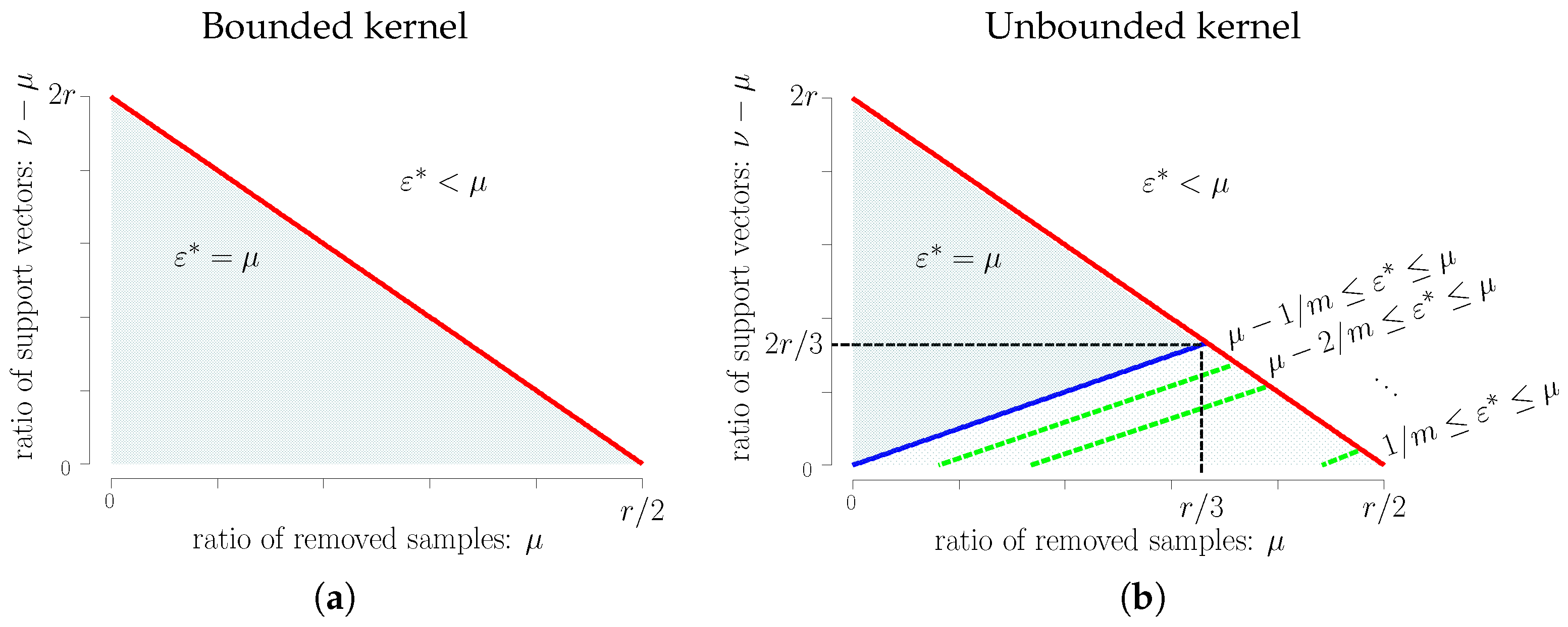
• Bounded kernel: For $\nu -\mu >2(r-2\mu )$, the breakdown point of $f_D\in \mathcal{H}$ is less than μ. For $\nu -\mu \le 2(r-2\mu )$, the breakdown point of $(f_D,b_D)$ is equal to μ.
• Unbounded kernel: For $\nu -\mu >2(r-2\mu )$, the breakdown point of $f_D\in \mathcal{H}$ is less than μ. For $2\mu <\nu -\mu \le 2(r-2\mu )$, the breakdown point of $(f_D,b_D)$ is equal to μ. When $0<\nu -\mu <min\{2\mu ,2(r-2\mu \left)\right\}$, the breakdown point of $f_D$ is equal to μ, and the breakdown point of $b_D$ is bounded from below by $\mu -\ell /m$ and from above by μ, where $\ell \in \mathbb{N}$ depends on ν and μ, as shown in Theorem 3.

Figure 2 shows the breakdown point of robust $(\nu ,\mu )$-SVM. The line $\nu -\mu =2(r-2\mu )$ is critical. For unbounded kernels, we only obtain a bound of the breakdown point.

Figure 2. (a) breakdown point of $(f_D,b_D)$ given by robust $(\nu ,\mu )$-SVM with bounded kernel; (b) breakdown point of $(f_D,b_D)$ given by robust $(\nu ,\mu )$-SVM with unbounded kernel.

4.3. Breakdown Point Revisited

Let us reconsider the breakdown point of learning methods.

4.3.1. Effective Case of Breakdown Point

Suppose that the function ${\widehat{f}}_D\in \mathcal{H}$ is obtained by a learning method using the dataset D. Learning methods are categorized into two types according to the norm of ${\widehat{f}}_D$. The first type is the learning methods satisfying ${sup}_{D^{\prime }}{\parallel {\widehat{f}}_{D^{\prime }}\parallel }_{\mathcal{H}}=\infty$, and the second type is the ones such that ${sup}_{D^{\prime }}{\parallel {\widehat{f}}_{D^{\prime }}\parallel }_{\mathcal{H}}<\infty$, where the supremum is taken over arbitrary dataset of size m, i.e., $D^{\prime }\in {\mathcal{D}}_m={(\mathcal{X}\times \{+1,-1\})}^m$.

For learning methods of the first type, the breakdown point indicates the number of outliers such that the estimator remains in a uniformly-bounded region. This is meaningful information about the robustness of the learning method. In this case, the larger breakdown point is regarded as a more robust method. As shown in Theorems 1 and 2, the robust $(\nu ,\mu )$-SVM is a learning method of the first type.

The second type implies that the hypothesis space of the learning method is bounded regardless of datasets. The C-SVM, robust C-SVM and ROD belong to learning methods of the second type. Indeed, given a labeled dataset $D=\{(x_i,y_i):i\in \left[m\right]\}$, the non-negative property of the hinge loss in C-SVM leads to:

$$\begin{array}{c}\hfill \frac{1}{2}\parallel {\widehat{f}}_D{\parallel }_{\mathcal{H}}^2\le \frac{1}{2}{\parallel {\widehat{f}}_D\parallel }_{\mathcal{H}}^2+C\sum _{i=1}^m{[1-y_i({\widehat{f}}_D\left(x_i\right)+{\widehat{b}}_D)]}_{+}\le mC,\end{array}$$

where the last inequality comes from the fact that the objective value at $f=0$ and $b=0$ is greater than or equal to the optimal value. Likewise, one can prove that robust C-SVM and ROD have the same property. In this case, the naive definition of the breakdown point shown in Section 4.1 is not adequate, because the boundary effect of the hypothesis set is not taken into account. In the general definition of the breakdown point, the boundary of the hypothesis space is taken into account [20] (Chapter 3.2.5).

In this paper, we focus on the breakdown point of learning algorithms of the first type. Then, the analysis based on the breakdown point suggests proper choices of hyperparameters $(\nu ,\mu )$ as shown in succeeding sections.

4.3.2. Other Robust Estimators

Robust statistical inference has been studied for a long time in mathematical statistics, and a number of robust estimators have been proposed for many kinds of statistical problems [20,34,35]. In mathematical analysis, one needs to quantify the influence of samples on estimators. Here, the influence function, change of variance and breakdown point are often used as measures of robustness. In the machine learning literature, these measures have been used to analyze the theoretical properties of SVM and its robust variants. In [36], the robustness of a learning algorithm using a convex loss function was investigated on the basis of an influence function defined over an RKHS. When the influence function is uniformly bounded on the RKHS, the learning algorithm is regarded to be robust against outliers. It was proven that the least squares loss provides a robust learning algorithm for classification problems in this sense [36].

From the standpoint of the breakdown point, however, convex loss functions do not provide robust estimators, as shown in [20] (Chapter 5.16). Yu et al. [14] proved that the breakdown point of a learning algorithm using clipped loss is greater than or equal to $1/m$ in regression problems. In Section 4.2, we show a detailed analysis of the breakdown point for robust $(\nu ,\mu )$-SVM.

5. Admissible Region for Learning Parameters

The theoretical analysis in Section 4.2 suggests that robust $(\nu ,\mu )$-SVM satisfying $0<\nu -\mu <2(r-2\mu )$ is a good choice for obtaining a robust classifier, especially when a bounded kernel is used. Here, r is the label ratio of the non-contaminated original data D, and usually, it is unknown in real-world data analysis. Thus, we need to estimate r from the contaminated dataset $D^{\prime }$.

If an upper bound of the outlier ratio is known to be $\tilde{\mu }$, we have $D^{\prime }\in {\mathcal{D}}_{\tilde{\mu }m}$, where ${\mathcal{D}}_{\tilde{\mu }m}$ is defined from D. Let $r^{\prime }$ be the label ratio of $D^{\prime }$. Then, the label ratio of the original dataset D should satisfy $r_{\mathrm{low}}\le r\le r_{\mathrm{up}}$, where $r_{\mathrm{low}}=max\{r^{\prime }-\tilde{\mu },0\}$ and $r_{\mathrm{up}}=min\{r^{\prime }+\tilde{\mu },1/2\}$. Let ${\mathsf{\Lambda }}_{\mathrm{low}}$ and ${\mathsf{\Lambda }}_{\mathrm{up}}$ be:

$$\begin{array}{c}\hfill \begin{array}{c}{\displaystyle {\mathsf{\Lambda }}_{\mathrm{low}}=\{(\nu ,\mu ):0\le \mu \le \tilde{\mu },0<\nu -\mu <2(r_{\mathrm{low}}-2\mu )\},}\hfill \\ {\displaystyle {\mathsf{\Lambda }}_{\mathrm{up}}=\{(\nu ,\mu ):0\le \mu \le \tilde{\mu },0<\nu -\mu <2(r_{\mathrm{up}}-2\mu )\}.}\hfill \end{array}\end{array}$$

Robust $(\nu ,\mu )$-SVM with $(\nu ,\mu )\in {\mathsf{\Lambda }}_{\mathrm{low}}$ reaches the breakdown point μ for any non-contaminated dataset D such that $D^{\prime }\in {\mathcal{D}}_{\mu m}$ for given $D^{\prime }$. On the other hand, the parameters $(\nu ,\mu )$ on the outside of ${\mathsf{\Lambda }}_{\mathrm{up}}$ are not necessary. Indeed, for any non-contaminated data D such that $D^{\prime }\in {\mathcal{D}}_{\tilde{\mu }m}$ for given $D^{\prime }$, the parameters $(\nu ,\mu )$ satisfying $\nu -\mu >2(r_{\mathrm{up}}-2\mu )$ do not yield a learning method that reaches the breakdown point μ.

When the upper bound $\tilde{\mu }$ is unknown, we set $\tilde{\mu }=r/2$. As shown in the comments after Theorem 1, the outlier ratio greater than $r/2$ can totally violate the statistical features of the original dataset. In such a case, we need to reconsider the observation process. For $\tilde{\mu }=r/2$, we obtain ${\overline{r}}_{\mathrm{low}}\le r\le {\overline{r}}_{\mathrm{up}}$, where ${\overline{r}}_{\mathrm{low}}=2r^{\prime }/3$ and ${\overline{r}}_{\mathrm{up}}=min\{2r^{\prime },1/2\}$. Hence, in the worst case, the admissible set of learning parameters ν and μ is:

$$\begin{array}{c}\hfill \begin{array}{c}{\displaystyle {\overline{\mathsf{\Lambda }}}_{\mathrm{low}}=\{(\nu ,\mu ):0<\nu -\mu <2({\overline{r}}_{\mathrm{low}}-2\mu )\},\mathrm{or}}\hfill \\ {\displaystyle {\overline{\mathsf{\Lambda }}}_{\mathrm{up}}=\{(\nu ,\mu ):0<\nu -\mu <2({\overline{r}}_{\mathrm{up}}-2\mu )\}.}\hfill \end{array}\end{array}$$

(16)

Given contaminated training data $D^{\prime }$, for any D of size m with a label ratio $r\in [{\overline{r}}_{\mathrm{low}},{\overline{r}}_{\mathrm{up}}]$, such that $D^{\prime }\in {\mathcal{D}}_{\mu m}$ with $\mu <{\overline{r}}_{\mathrm{low}}/2$, robust $(\nu ,\mu )$-SVM with $(\nu ,\mu )\in {\overline{\mathsf{\Lambda }}}_{\mathrm{low}}$ provides a classifier with the breakdown point μ. A parameter $(\nu ,\mu )$ on the outside of ${\overline{\mathsf{\Lambda }}}_{\mathrm{up}}$ is not necessary, for the same reasons as for ${\mathsf{\Lambda }}_{\mathrm{up}}$.

The admissible region of $(\nu ,\mu )$ is useful when the parameters are determined by a grid search based on cross-validation. On the other hand, C of robust C-SVM and λ in ROD can take a wide range of positive real numbers. Hence, differently from robust $(\nu ,\mu )$-SVM, these algorithms need heuristics to determine the region of the grid search for the learning parameters.

The numerical experiments presented in Section 6 applied a grid search to the region ${\overline{\mathsf{\Lambda }}}_{\mathrm{up}}$.

6. Numerical Experiments

We conducted numerical experiments on synthetic and benchmark datasets to compare a number of SVMs. Algorithm 1 was used for robust $(\nu ,\mu )$-SVM, and DCA in [12] was used for robust C-SVM with the ramp loss. We used CPLEX to solve the convex quadratic problems.

6.1. DCA versus Global Optimization Methods

As has been shown in many studies including [37], DCA quite often gives global optimal solutions to many different and various non-convex optimization problems. We examined how often DCA produces global optimal solutions to robust $(\nu ,\mu )$-SVM with the 0-1 valued outlier indicator. Here, the numerical solution of DCA in robust $(\nu ,\mu )$-SVM denotes the output of Step 5 in Algorithm 1. In these numerical experiments, the optimization problem was formulated as a mixed integer programming (MIP) problem, and the CPLEX MIP solver was used to compute the global optimal solution of robust $(\nu ,\mu )$-SVM based on a relatively small dataset. The numerical solution given by DCA was compared with the global optimal solution.

In binary classification problems, positive (resp. negative) samples were generated from a multivariate normal distribution with mean ${\mu }_p=1_d\in {\mathbb{R}}^d$ (resp. ${\mu }_n=-1_d\in {\mathbb{R}}^d$) and a variance-covariance matrix $cI$, where I is the identity matrix and c is a positive constant. Each class had 20 samples. For such a small dataset, the global optimal solution was obtained by the CPLEX MIP solver. Outliers were added by flipping positive labels randomly, and the outlier ratio was $10\%$. The DCA with the multi-start method was used to solve the robust $(\nu ,\mu )$-SVM using the linear kernel. In the multi-start method, a number of initial points were randomly generated, and for each initial point, a numerical solution was obtained by DCA. Among these numerical solutions, the point that attained the smallest objective value was chosen as the output of the multi-start method. $\mathrm{opt}\left(\mathrm{DCA}\right)$ was the objective value at the numerical solution of DCA, and $\mathrm{opt}\left(\mathrm{MIP}\right)$ was the global optimal value. Note that the optimal value of the problem in robust $(\nu ,\mu )$-SVM is non-positive, i.e., $\mathrm{opt}\left(\mathrm{MIP}\right)\le 0$. In addition, one can find that any numerical solution obtained by DCA satisfies $\mathrm{opt}\left(\mathrm{DCA}\right)\le 0$.

In the numerical experiments, 100 training datasets such that $\mathrm{opt}\left(\mathrm{MIP}\right)<-{10}^{-4}$ were randomly generated, and $\mathrm{opt}\left(\mathrm{DCA}\right)$ was computed for each dataset. Table 1 shows the number of times that $\mathrm{opt}\left(\mathrm{DCA}\right)/\mathrm{opt}\left(\mathrm{MIP}\right)\ge 0.97$ holds out of 100 trials. When the achievable lowest test error, i.e., the Bayes error, was large, the DCA tended to yield a local optimal solution that was not globally optimal. When the Bayes error was small, DCA produced approximately global optimal solutions in almost all trials. Even when DCA using a single initial point failed to find the global optimal solution, the multi-start method with five or 10 initial points greatly improved the quality of the numerical solutions. In numerical experiments, DCA was more than 50 times more computationally efficient than the MIP solver.

Table 1. Number of times that the numerical solution of difference of convex functions algorithm (DCA) satisfies $\mathrm{opt}\left(\mathrm{DCA}\right)/\mathrm{opt}\left(\mathrm{MIP}\right)\ge 0.97$ out of 100 trials. The number of initial points used in the multi-start method is denoted as #initial points. The“Dim.” and “Cov.” columns denote the dimension d and the covariance matrix of the input vectors in each label. The column labeled “Err.” shows the Bayes error of each problem setting.

Setting		Err. (%)	$(\mathit{\nu },\mathit{\mu })$ in Robust $(\mathit{\nu },\mathit{\mu })$-SVM Using Linear Kernel
			$(0.4,0.1)$			$(0.5,0.1)$			$(0.6,0.1)$
Dim.	Cov.		#Initial Points			#Initial Points			#Initial Points
			1	5	10	1	5	10	1	5	10
2	I	7.9	87	96	97	90	99	99	93	99	99
5	I	1.3	98	99	100	100	100	100	99	100	100
10	I	0.1	100	100	100	100	100	100	100	100	100
2	$5I$	26.4	78	84	88	76	85	90	75	85	86
5	$10I$	24.0	46	84	90	53	83	90	66	90	90
10	$50I$	32.7	16	59	73	31	72	77	46	85	92

6.2. Computational Cost

We conducted numerical experiments to compare the computational cost of robust $(\nu ,\mu )$-SVM with that of robust C-SVM. Both learning algorithms employed the DCA. The numerical experiments were conducted on AMD Opteron Processors 6176 (2.3 GHz) with 48 cores, running Cent OS Linux Release 6.4. We used three benchmark datasets, Sonar, BreastCancer and spam, which were also used in the experiments in Section 6.5. m training samples were randomly chosen from each dataset, and each dataset was contaminated by outliers. The outlier ratio was $5\%$, and outliers were added by flipping the labels randomly. Robust $(\nu ,\mu )$-SVM and robust C-SVM with the linear kernel were used to obtain classifiers from the contaminated datasets. This process was repeated 20 times for each dataset. Table 2 presents the average computation time and average ratio of support vectors (SV ratio) together with standard deviations. The support vector was numerically identified as the data point $x_i$ having the coefficient ${\alpha }_i$ such that $|{\alpha }_i|$ is greater than ${10}^{-10}$. Although the SV ratio is bounded below by $\nu -\mu$, the bound was not necessarily tight. A similar tendency is often observed in ν-SVM. In terms of the computation time, two learning algorithms were not significantly different except in the case of robust C-SVM with a small C that induces a strong regularization.

Table 2. Computation time (Time) and ratio of support vectors (SV Ratio) of robust $(\nu ,\mu )$-SVM and robust C-SVMwith standard deviations.

Linear Kernel	Sonar ($\mathit{m}=104$)		BreastCancer ($\mathit{m}=350$)		Spam ($\mathit{m}=1000$)
Robust $(\mathit{\nu },\mathit{\mu })$-SVM, $(\mathit{\nu },\mathit{\mu })$	Time (s)	SV Ratio	Time (s)	SV Ratio	Time (s)	SV Ratio
$(0.2,0.10)$	1.10 (0.22)	0.79 (0.14)	1.02 (0.17)	0.21 (0.11)	13.38 (3.90)	0.27 (0.22)
$(0.2,0.05)$	0.87 (0.15)	0.75 (0.20)	0.73 (0.13)	0.18 (0.06)	11.29 (2.41)	0.64 (0.27)
$(0.3,0.10)$	1.17 (0.19)	0.57 (0.12)	0.80 (0.13)	0.22 (0.07)	9.65 (2.13)	0.24 (0.04)
$(0.3,0.05)$	0.81 (0.09)	0.58 (0.16)	0.63 (0.07)	0.28 (0.05)	8.64 (2.12)	0.36 (0.21)
$(0.4,0.10)$	1.11 (0.18)	0.49 (0.10)	0.83 (0.14)	0.30 (0.03)	8.65 (1.25)	0.30 (0.02)
$(0.4,0.05)$	0.90 (0.15)	0.62 (0.16)	0.76 (0.12)	0.36 (0.02)	8.72 (1.77)	0.38 (0.04)
Robust $\mathit{C}$-SVM, $\mathit{C}$
${10}^{-7}$	0.12 (0.02)	0.00 (0.00)	0.15 (0.02)	0.00 (0.00)	1.62 (0.08)	0.00 (0.00)
1	0.61 (0.07)	0.45 (0.08)	0.60 (0.16)	0.04 (0.01)	7.38 (2.36)	0.08 (0.01)
${10}^7$	1.02 (0.11)	0.54 (0.13)	0.68 (0.18)	0.03 (0.01)	10.16 (3.31)	0.11 (0.16)
${10}^{12}$	1.07 (0.13)	0.47 (0.09)	0.63 (0.17)	0.05 (0.06)	20.98 (5.95)	0.30 (0.32)

6.3. Outlier Detection

Robust $(\nu ,\mu )$-SVM uses an outlier indicator to suppress the influence of outliers. Figure 3 shows that the outlier indicator in the robust $(\nu ,\mu )$-SVM using the linear kernel is able to detect outliers in a synthetic setting. Similar results have been reported for learning methods using outlier indicators such as ROD and ER-SVM. Systematic experiments using a recall-precision criterion were presented in [17,19].

Figure 3. Plot of contaminated dataset of size $m=200$. The outlier ratio is $0.05$, and the asterisks (∗) denote the outlier. In the panels of the upper (resp. lower) row, outliers are added by flipping labels (resp. flipping positive labels) randomly. The dashed line is the true decision boundary, and the solid line is the decision boundary estimated using ν-SVM with $\nu =0.3$ in (a,d); robust $(\nu ,\mu )$-SVM with $(\nu ,\mu )=(0.3,0.05)$ in (b,e); and $(\nu ,\mu )=(0.3,0.1)$ in (c,f). The triangles denote the samples on which ${\eta }_i=0$ is assigned.

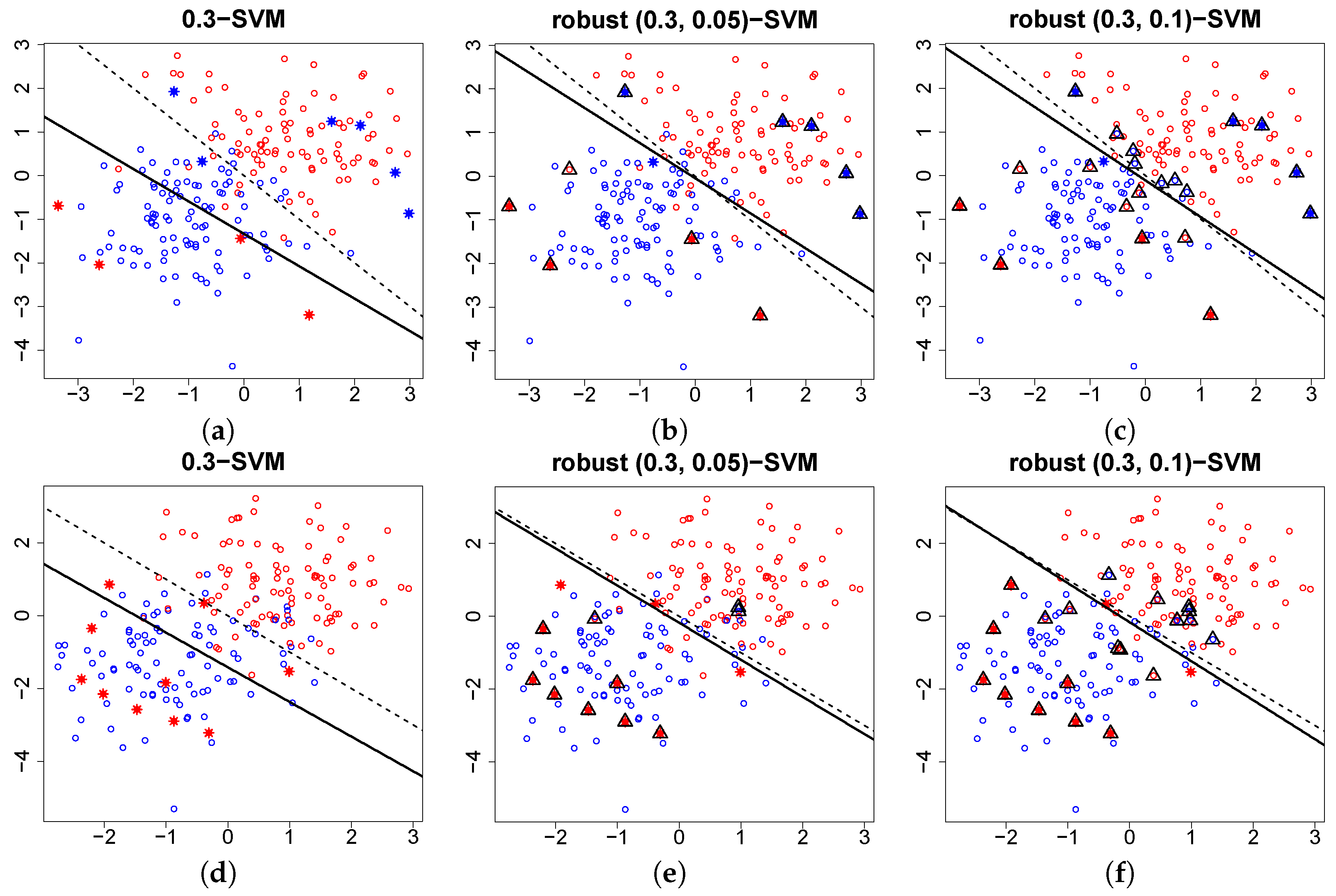
6.4. Breakdown Point

We investigate the validity of Inequality (14) in Theorem 1. In the numerical experiments, the original data D were generated using mlbench.spiralsin the mlbench library of the R language [38]. Given an outlier ratio μ, positive samples of size $\mu m$ were randomly chosen from D, and they were replaced with randomly-generated outliers to obtain a contaminated dataset $D^{\prime }\in {\mathcal{D}}_{\mu m}$. The original data D and an example of the contaminated data $D^{\prime }\in {\mathcal{D}}_{\mu m}$ are shown in Figure 4. The decision function $g\left(x\right)=f\left(x\right)+b$ was estimated from $D^{\prime }$ by using robust $(\nu ,\mu )$-SVM. Here, the true outlier ratio μ was used as the parameter of the learning algorithm. The norms of f and b were then calculated. The above process was repeated 30 times for each pair of parameters $(\nu ,\mu )$, and the maximum values of ${\parallel f\parallel }_{\mathcal{H}}$ and $\left|b\right|$ were computed.

Figure 4. (a) original data D; (b) contaminated data $D^{\prime }\in {\mathcal{D}}_{\mu m}$. In this example, the sample size is $m=200$, and the outlier ratio is $\mu =0.1$.

Figure 5 shows the results of the numerical experiments. The maximum norm of the estimated decision function is plotted for the parameter $(\mu ,\nu -\mu )$ on the same axis as in Figure 2. The top (bottom) panels show the results for a Gaussian (linear) kernel. The left and middle columns show the maximum norm of f and b, respectively. The maximum test errors are presented in the right column. In all panels, the red points denote the top 50 percent of values, and the asterisks (∗) are the point that violates the inequality $\nu -\mu \le 2(r-2\mu )$. In this example, the numerical results agree with the theoretical analysis in Section 4; i.e., the norm becomes large when the inequality $\nu -\mu \le 2(r-2\mu )$ is violated. Accordingly, the test error gets close to $0.5$; no information for classification. Even when the unbounded linear kernel is used, robustness is confirmed for the parameters in the left lower region in the right panel of Figure 2.

Figure 5. Plots of maximum norms and worst-case test errors. The top (Bottom) panels show the results for a Gaussian (linear) kernel. Red points mean the top 50 percent of values; the asterisks (∗) are points that violate the inequality $\nu -\mu \le 2(r-2\mu )$. (a) Gaussian kernel; (b) linear kernel.

In the bottom right panel, the test error gets large when the inequality $\nu -\mu \le 2(r-2\mu )$ holds. This result comes from the problem setup. Even with non-contaminated data, the test error of the standard ν-SVM is approximately $0.5$, because the linear kernel works poorly for spiral data. Thus, the worst-case test error under the target distribution can go beyond $0.5$. For the parameter at which (14) is violated, the test error is always close to $0.5$. Thus, a learning method with such parameters does not provide any useful information for classification.

6.5. Prediction Accuracy

As shown in Section 5, the theoretical analysis of the breakdown point yields the admissible region, such as ${\overline{\mathsf{\Lambda }}}_{\mathrm{up}}$, for learning parameters in robust $(\nu ,\mu )$-SVM. Learning parameters outside the admissible region produce an unstable learning algorithm. Hence, one can reduce the computational cost of tuning the learning parameters by ignoring outside of the admissible region. In this section, we verify the usefulness of the admissible region.

We compared the generalization ability of robust $(\nu ,\mu )$-SVM with ν-SVM and robust C-SVM using the ramp loss. In robust $(\nu ,\mu )$-SVM, a grid search of the region ${\overline{\mathsf{\Lambda }}}_{\mathrm{up}}$ is used to choose the learning parameters, ν and μ.

The datasets are presented in Table 3. The datasets are from the mlbench and kernlab libraries of the R language [38]. The number of positive samples in these datasets is less than or equal to the number of negative samples. Before running the learning algorithms, we standardized each input variable to be mean zero and standard deviation one.

Table 3. Test error and standard deviation of robust $(\nu ,\mu )$-SVM, robust C-SVM and ν-SVM. The dimension of the input vector, number of training samples, number of test samples and label ratio of all samples with no outliers are shown for each dataset. Linear and Gaussian kernels were used to build the classifier in each method. The outlier ratio in the training data ranged from 0% to 15%, and the test error was evaluated on the non-contaminated test data. The asterisks (*) mean the best result for a fixed kernel function in each dataset, and the double asterisks (**) mean that the corresponding method is 5% significant compared with the second best method under a one-sided t-test. The learning parameters were determined by five-fold cross-validation on the contaminated training data.

Data	Outlier	Linear Kernel			Gaussian Kernel
		Robust $(\mathit{\nu },\mathit{\mu })$-SVM	Robust C-SVM	ν-SVM	Robust $(\mathit{\nu },\mathit{\mu })$-SVM	Robust C-SVM	ν-SVM
Sonar: $dimx=60$,	0%	*0.258(.032)	0.270(.038)	* 0.256(.051)	* 0.179(.038)	**0.188(0.043)	*0.181(0.039)
$\#Train=104$,	5%	* 0.256(0.039)	0.273(0.047)	*0.258(0.046)	*0.225(0.042)	**0.229(0.051)	* 0.224(0.061)
$\#Test=104$,	10%	* 0.297(0.060)	0.306(0.067)	*0.314(0.060)	*0.249(0.059)	** 0.230(0.046)	*0.259(0.062)
$r=0.466$.	15%	* 0.329(0.061)	0.339(0.064)	*0.345(0.062)	*0.280(0.053)	** 0.280(0.050)	*0.294(0.064)
BreastCancer: $dimx=10$,	0%	0.033(.010)	*0.035(0.008)	* 0.033(0.006)	** 0.032(0.008)	*0.035(0.012)	0.033(0.010)
$\#train=350$,	5%	0.034(0.009)	* 0.034(0.010)	*0.043(0.015)	** 0.032(.005)	*0.033(0.007)	0.033(0.006)
$\#test=349$,	10%	0.055(0.015)	* 0.051(0.026)	*0.076(0.036)	** 0.035(0.008)	*0.043(0.025)	0.038(0.008)
$r=0.345$	15%	0.136(0.058)	* 0.120(0.050)	*0.148(0.058)	**0.160(0.083)	* 0.145(0.070)	0.150(0.110)
PimaIndiansDiabetes:	0%	**0.237(0.018)	* 0.232(0.014)	0.246(0.018)	* 0.238(0.021)	*0.240(0.019)	0.243(0.022)
$dimx=8$, $\#train=384$,	5%	**0.239(0.019)	* 0.237(0.016)	0.269(0.036)	* 0.264(0.025)	*0.267(0.024)	0.273(0.024)
$\#test=384$,	10%	** 0.280(0.046)	*0.299(0.042)	0.330(0.030)	*0.302(0.039)	* 0.293(0.036)	0.315(0.038)
$r=0.349$	15%	** 0.338(0.042)	*0.349(0.030)	0.351(0.026)	* 0.344(0.028)	*0.344(0.031)	0.353(0.016)
spam: $dimx=57$,	0%	**0.083(0.005)	0.088(0.006)	*0.083(0.005)	**0.081(0.005)	0.086(0.006)	* 0.081(0.006)
$\#train=1000$,	5%	** 0.094(0.008)	0.104(0.013)	*0.109(0.010)	**0.095(0.008)	0.097(0.009)	* 0.095(0.008)
$\#test=3601$,	10%	** 0.129(0.022)	0.152(0.020)	*0.166(0.067)	** 0.129(0.015)	0.133(0.017)	0.141(.030)
$r=0.394$	15%	** 0.201(0.029)	0.240(0.030)	*0.256(0.091)	** 0.206(0.018)	0.223(0.030)	0.240(0.055)
Satellite: $dimx=36$,	0%	**0.097(0.004)	*0.096(0.003)	** 0.094(0.003)	*0.069(0.031)	0.067(0.004)	** 0.063(0.004)
$\#train=2000$,	5%	**0.101(0.003)	* 0.100(0.005)	**0.100(0.004)	*0.072(0.015)	0.078(0.007)	**0.078(0.043)
$\#test=4435$, $r=0.234$	10%	** 0.148(0.020)	*0.161(0.026)	**0.161(0.019)	*0.117(0.034)	0.126(0.040)	**0.137(0.027)

We randomly split the dataset into training and test sets. To evaluate the robustness, the training data were contaminated by outliers. More precisely, we randomly chose positive labeled samples in the training data and changed their labels to negative; i.e., we added outliers by flipping the labels. After that, robust $(\nu ,\mu )$-SVM, robust C-SVM using the ramp loss and the standard ν-SVM were used to obtain classifiers from the contaminated training dataset. The prediction accuracy of each classifier was evaluated over test data that had no outliers. Linear and Gaussian kernels were employed for each learning algorithm. The learning parameters, such as $\mu ,\nu$ and C, were determined by conducting a grid search based on five-fold cross-validation over the training data. For robust $(\nu ,\mu )$-SVM, the parameter $(\mu ,\nu )$ was selected from the admissible region ${\overline{\mathsf{\Lambda }}}_{\mathrm{up}}$ in (16). For standard ν-SVM, the candidate of the regularization parameter ν was selected from the interval $(0,2r^{\prime })$, where $r^{\prime }$ is the label ratio of the contaminated training data. For robust C-SVM, the regularization parameter C was selected from the interval $[{10}^{-7},{10}^7]$. In the grid search of the parameters, 24 or 25 candidates were examined for each learning method. Thus, we needed to solve convex or non-convex optimization problems more than $24\times 5$ times in order to obtain a classifier. The above process was repeated 30 times, and the average test error was calculated.

The results are presented in Table 3. For non-contaminated training data, robust $(\nu ,\mu )$-SVM and robust C-SVM were comparable to the standard ν-SVM. When the outlier ratio is high, we can conclude that robust $(\nu ,\mu )$-SVM and robust C-SVM tend to work better than the standard ν-SVM. In this experiment, the kernel function does not affect the relative prediction performance of these learning methods. In large datasets, such as spam and Satellite, robust $(\nu ,\mu )$-SVM tends to outperform robust C-SVM. When the learning parameters, such as $\nu ,\mu$ and C, are appropriately chosen by using a large dataset, the learning algorithms with multiple learning parameters clearly work better than those with a single learning parameter. In addition, in robust C-SVM, there is a difficulty in choosing the regularization parameter. Indeed, the parameter C does not have a clear meaning, and thus, it is not so easy to determine its candidates in the grid search optimization. In contrast, ν in ν-SVM and its robust variant has a clear meaning, i.e., a lower bound of the ratio of support vectors and an upper bound of the margin error on the training data [5]. Such a clear meaning is helpful for choosing candidate points of regularization parameters.

7. Concluding Remarks

We have investigated the breakdown point of robust variants of SVMs. The theoretical analysis provides inequalities of learning parameters, ν and μ, in robust $(\nu ,\mu )$-SVM that guarantee the robustness of the learning algorithm. Numerical experiments showed that the inequalities are critical to obtaining a robust classifier. The exact evaluation of the breakdown point for robust $(\nu ,\mu )$-SVM enables us to restrict the range of the learning parameters and to increase the chance of finding a robust classifier with good performance for the same computational cost.

In our paper, the dual representation of robust SVMs is applied to the calculation of the breakdown point. Theoretical analysis using the dual representation can be a powerful tool for the detailed analysis of other learning algorithms.

On the theoretical side, it is interesting to establish the relationship between the robustness, say breakdown point, and the convergence speed of learning algorithms, as presented for the parametric inference in mathematical statistics [34] (Chapter 2.4). Furthermore, it is important to determine the optimal parameter choice of $(\nu ,\mu )$ in robust $(\nu ,\mu )$-SVM as an extension of the parameter choice for ν-SVM [39]. Another important issue is to develop efficient optimization algorithms. Although the DC algorithm [12,27] and convex relaxation [14,17] are promising methods, more scalable algorithms will be required to deal with massive datasets that are often contaminated by outliers. Recently, a computationally-efficient algorithm, called iteratively weighted SVM (IWSVM), was developed to solve optimization problems in the robust C-SVM and its variants [40]. Moreover, a fixed point of IWSVM is assured to be a local optimal solution obtained by the DC algorithm. It will be worthwhile to investigate the applicability of IWSVM to robust $(\nu ,\mu )$-SVM.

References

- Cortes, C.; Vapnik, V. Support-vector networks. Mach. Learn. 1995, 20, 273–297. [Google Scholar] [CrossRef]
- Schölkopf, B.; Smola, A.J. Learning with Kernels; MIT Press: Cambridge, MA, USA, 2002. [Google Scholar]
- Berlinet, A.; Thomas-Agnan, C. Reproducing Kernel Hilbert Spaces in Probability and Statistics; Kluwer Academic: Boston, MA, USA, 2004. [Google Scholar]
- Perez-Cruz, F.; Weston, J.; Hermann, D.J.L.; Schölkopf, B. Extension of the ν-SVM Range for Classification. In Advances in Learning Theory: Methods, Models and Applications 190; IOS Press: Amsterdam, The Netherlands, 2003; pp. 179–196. [Google Scholar]
- Schölkopf, B.; Smola, A.; Williamson, R.; Bartlett, P. New support vector algorithms. Neural Comput. 2000, 12, 1207–1245. [Google Scholar] [CrossRef] [PubMed]
- Suykens, J.A.K.; Vandewalle, J. Least squares support vector machine classifiers. Neural Process. Lett. 1999, 9, 293–300. [Google Scholar] [CrossRef]
- Bartlett, P.L.; Jordan, M.I.; McAuliffe, J.D. Convexity, classification, and risk bounds. J. Am. Stat. Assoc. 2006, 101, 138–156. [Google Scholar] [CrossRef]
- Steinwart, I. On the influence of the kernel on the consistency of support vector machines. J. Mach. Learn. Res. 2001, 2, 67–93. [Google Scholar]
- Zhang, T. Statistical behavior and consistency of classification methods based on convex risk minimization. Ann. Stat. 2004, 32, 56–134. [Google Scholar] [CrossRef]
- Shen, X.; Tseng, G.C.; Zhang, X.; Wong, W.H. On ψ-learning. J. Am. Stat. Assoc. 2003, 98, 724–734. [Google Scholar] [CrossRef]
- Yu, Y.; Yang, M.; Xu, L.; White, M.; Schuurmans, D. Relaxed Clipping: A Global Training Method for Robust Regression and Classification. In Neural Information Processing Systems; MIT Press: Cambridge, MA, USA, 2010; pp. 2532–2540. [Google Scholar]
- Collobert, R.; Sinz, F.; Weston, J.; Bottou, L. Trading Convexity for Scalability. In Proceedings of the ICML06, 23rd International Conference on Machine Learning, Pittsburgh, PA, USA, 25–29 June 2006; ACM Press: New York, NY, USA, 2006; pp. 201–208. [Google Scholar]
- Wu, Y.; Liu, Y. Robust truncated hinge loss support vector machines. J. Am. Stat. Assoc. 2007, 102, 974–983. [Google Scholar] [CrossRef]
- Yu, Y.; Aslan, Ö.; Schuurmans, D. A Polynomial-Time Form of Robust Regression. In Advances in Neural Information Processing Systems 25; Curran Associates, Inc.: Red Hook, NY, USA, 2012; pp. 2483–2491. [Google Scholar]
- Feng, Y.; Yang, Y.; Huang, X.; Mehrkanoon, S.; Suykens, J.A. Robust Support Vector Machines for Classification with Nonconvex and Smooth Losses. Neural Comput. 2016, 28, 1217–1247. [Google Scholar] [CrossRef] [PubMed]
- Tsyurmasto, P.; Uryasev, S.; Gotoh, J. Support Vector Classification with Positive Homogeneous Risk Functionals; Technical Report, Research Report 2013-4; Department of Industrial and Systems Engineering, University of Florida: Gainesville, FL, USA, 2013. [Google Scholar]
- Xu, L.; Crammer, K.; Schuurmans, D. Robust Support Vector Machine Training Via Convex Outlier Ablation. In Proceedings of the AAAI, Boston, MA, USA, 16–20 July 2006; pp. 536–542.
- Fujiwara, S.; Takeda, A.; Kanamori, T. DC Algorithm for Extended Robust Support Vector Machine; Technical Report METR 2014–38; The University of Tokyo: Tokyo, Japan, 2014. [Google Scholar]
- Takeda, A.; Fujiwara, S.; Kanamori, T. Extended robust support vector machine based on financial risk minimization. Neural Comput. 2014, 26, 2541–2569. [Google Scholar] [CrossRef] [PubMed]
- Maronna, R.; Martin, R.D.; Yohai, V. Robust Statistics: Theory and Methods; Wiley: Hoboken, NJ, USA, 2006. [Google Scholar]
- Schapire, R.E.; Freund, Y.; Bartlett, P.L.; Lee, W.S. Boosting the margin: A new explanation for the effectiveness of voting methods. Ann. Stat. 1998, 26, 1651–1686. [Google Scholar] [CrossRef]
- Kimeldorf, G.S.; Wahba, G. Some results on Tchebycheffian spline functions. J. Math. Anal. Appl. 1971, 33, 82–95. [Google Scholar] [CrossRef]
- Wahba, G. Advances in Kernel Methods; Chapter Support Vector Machines, Reproducing Kernel Hilbert Spaces, and Randomized GACV; MIT Press: Cambridge, MA, USA, 1999; pp. 69–88. [Google Scholar]
- Takeda, A.; Sugiyama, M. ν-Support Vector Machine as Conditional Value-at-Risk Minimization. In Proceedings of the ICML, ACM International Conference Proceeding Series, Yokohama, Japan, 3–5 December 2008; Cohen, W.W., McCallum, A., Roweis, S.T., Eds.; ACM: New York, NY, USA, 2008; Volume 307, pp. 1056–1063. [Google Scholar]
- Rockafellar, R.T.; Uryasev, S. Conditional value-at-risk for general loss distributions. J. Bank. Financ. 2002, 26, 1443–1472. [Google Scholar] [CrossRef]
- Boyd, S.; Vandenberghe, L. Convex Optimization; Cambridge University Press: Cambridge, UK, 2004. [Google Scholar]
- Le Thi, H.A.; Dinh, T.P. Convex analysis approach to d.c. programming: Theory, algorithms and applications. Acta Math. Vietnam. 1997, 22, 289–355. [Google Scholar]
- Yuille, A.L.; Rangarajan, A. The concave-convex procedure. Neural Comput. 2003, 15, 915–936. [Google Scholar] [CrossRef] [PubMed]
- Crisp, D.J.; Burges, C.J.C. A Geometric Interpretation of ν-SVM Classifiers. In Advances in Neural Information Processing Systems 12; Solla, S.A., Leen, T.K., Müller, K.-R., Eds.; MIT Press: Cambridge, MA, USA, 2000; pp. 244–250. [Google Scholar]
- Kanamori, T.; Takeda, A.; Suzuki, T. Conjugate relation between loss functions and uncertainty sets in classification problems. J. Mach. Learn. Res. 2013, 14, 1461–1504. [Google Scholar]
- Takeda, A.; Mitsugi, H.; Kanamori, T. A Unified Robust Classification Model. In Proceedings of the 29th International Conference on Machine Learning (ICML-12), ICML’12, Edinburgh, Scotland, 26 June–1 July 2012; Langford, J., Pineau, J., Eds.; Omnipress: New York, NY, USA, 2012; pp. 129–136. [Google Scholar]
- Bertsekas, D.; Nedic, A.; Ozdaglar, A. Convex Analysis and Optimization; Athena Scientific: Belmont, MA, USA, 2003. [Google Scholar]
- Donoho, D.; Huber, P. The Notion of Breakdown Point. In A Festschrift for Erich L. Lehmann; CRC Press: Boca Raton, FL, USA, 1983; pp. 157–184. [Google Scholar]
- Hampel, F.R.; Rousseeuw, P.J.; Ronchetti, E.M.; Stahel, W.A. Robust Statistics. The Approach Based on Influence Functions; John Wiley and Sons, Inc.: Hoboken, NJ, USA, 1986. [Google Scholar]
- Huber, P.J.; Ronchetti, E.M. Robust Statistics, 2nd ed.; Wiley: New York, NY, USA, 2009. [Google Scholar]
- Christmann, A.; Steinwart, I. On robustness properties of convex risk minimization methods for pattern recognition. J. Mach. Learn. Res. 2004, 5, 1007–1034. [Google Scholar]
- Le Thi, H.A.; Dinh, T.P. The DC (Difference of Convex Functions) Programming and DCA Revisited with DC Models of Real World Nonconvex Optimization Problems. Ann. Oper. Res. 2005, 133, 23–46. [Google Scholar]
- R Core Team. R: A Language and Environment for Statistical Computing; R Foundation for Statistical Computing: Vienna, Austria, 2014. [Google Scholar]
- Steinwart, I. On the optimal parameter choice for ν-support vector machines. IEEE Trans. Pattern Anal. Mach. Intell. 2003, 25, 1274–1284. [Google Scholar] [CrossRef]
- Wu, Y.; Liu, Y. Adaptively weighted large margin classifiers. J. Comput. Graph. Stat. 2013, 22, 416–432. [Google Scholar] [CrossRef] [PubMed]
© 2017 by the authors. Licensee MDPI, Basel, Switzerland. This article is an open access article distributed under the terms and conditions of the Creative Commons Attribution (CC BY) license ( http://creativecommons.org/licenses/by/4.0/).