1. Introduction
Finite population evolutionary dynamics are of broad interest for both application and theory [
1,
2,
3,
4,
5,
6,
7,
8]; in particular, concepts of evolutionary stability have been widely-studied [
6,
7,
8,
9], and recently applied to finite populations [
10] with mutation (and weak selection) [
11]. Many evolutionary dynamics, such as the replicator equation, effectively assume infinite population sizes which allows a variety of tools from dynamical systems to be applied. Lyapunov stability theorems are crucial tools in the study of dynamical systems and evolutionary dynamics and there is a long history of Lyapunov stability results in evolutionary game theory and mathematical biology [
8,
12,
13,
14,
15]. Evolutionary dynamics in finite populations are commonly modeled as Markov processes, such as the Moran and the Wright–Fisher processes [
16,
17,
18,
19,
20], which are not deterministic; in the case of the Moran process, the replicator equation can be recovered in a large population limit [
21,
22]. Such stochastic models lack Lyapunov stability theorems. The theory of Markov processes, however, provides powerful analytic tools, notably the stationary distribution, capturing the long-run behavior of a process. We will show that there is an intimate connection between the stationary distributions of these processes and the celebrated theory of evolutionary stability. See
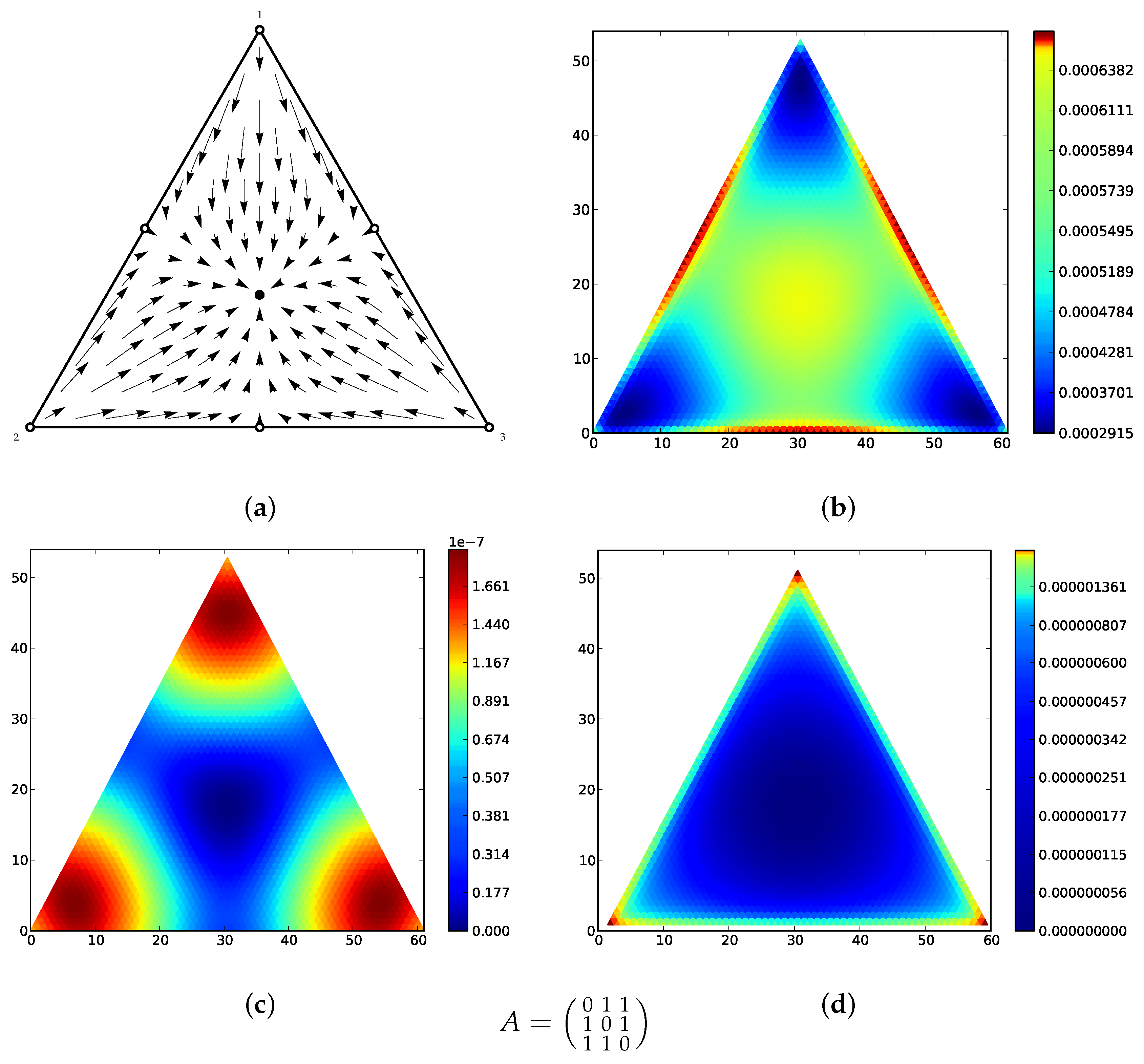
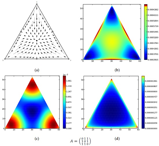
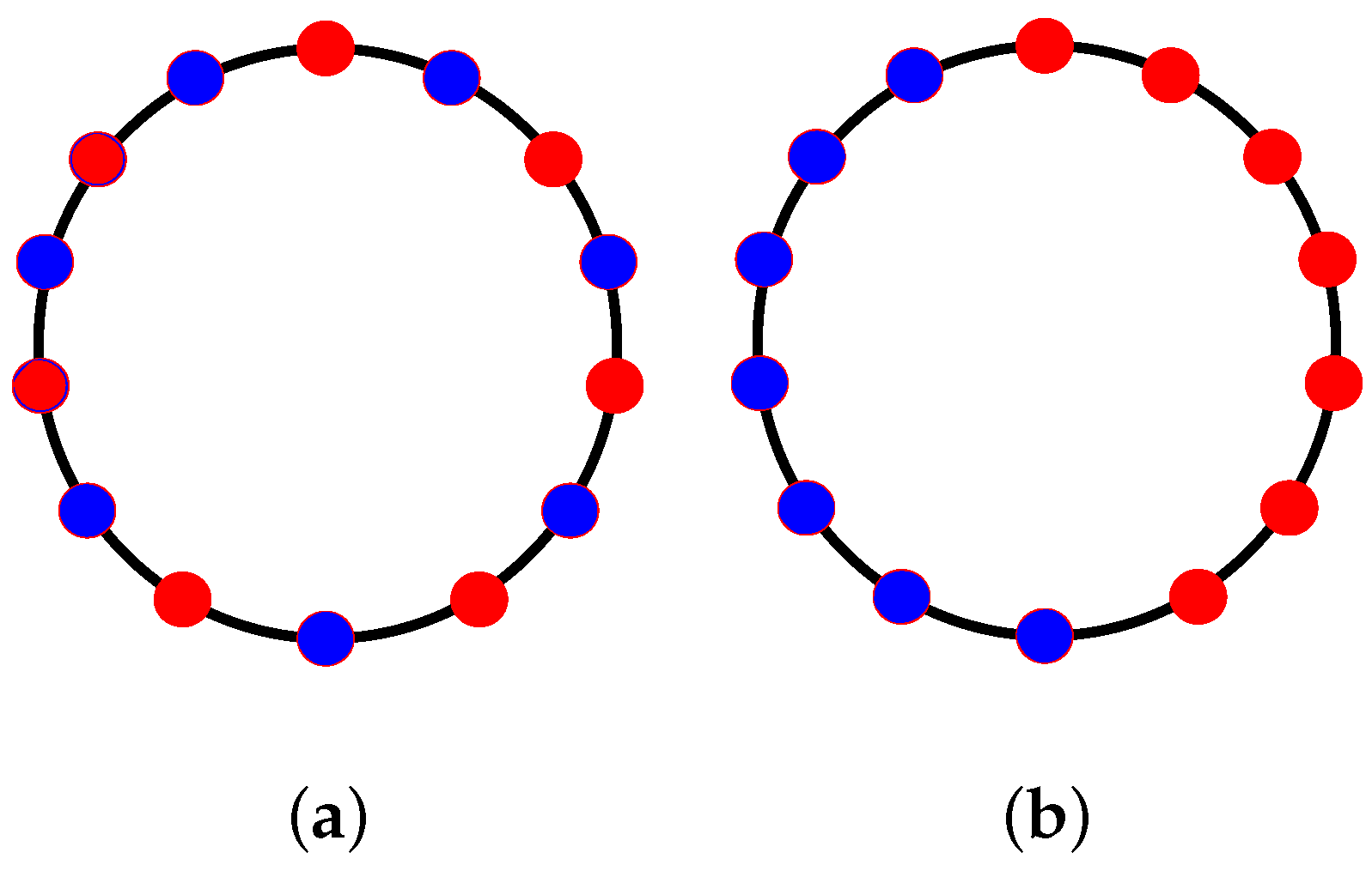
Figure 1 for a motivating example of the main theorem in a population of three types.
In particular, for populations of finitely many replicating types, we define a
Lyapunov-like quantity, namely a quantity that is positive-definite, decreasing toward an “equilibrium” locally, and minimal at the equilibrium, for a large class of birth-death processes we call the incentive process [
24], including the Moran process and the Fermi process [
25]. We then show local maxima of the stationary distribution of the Markov processes are local minima of the Lyapunov quantity for sufficiently large populations, which in turn are generalized evolutionarily stable states. In this manner, we have effectively extended the folk theorem of evolutionary dynamics [
26,
27] to these stochastic processes, including those with mutation (in fact we generally require some mutation for the stationary distribution to exist). Similar yet more nuanced results hold for the Wright–Fisher process on two types. For dynamics on populations of three types, such as the famous rock-scissors-paper dynamics, we show that similar results hold for the Moran process, and that the stationary distribution and Lyapunov quantity recapitulate the phase portraits of the replicator equation. Our main results apply to populations with any finite number of types. Finally we demonstrate some extensions to the dynamics of birth-death processes in structured populations, i.e., in the context of evolutionary graph theory, and of populations of variable size.
The use of information-theoretic quantities such as cross entropy and relative entropy [
28] date back at least to [
12] and [
13]. Recently author Harper used generalizations from statistical thermodynamics [
29] to extend the well-known Lyapunov stability result for the replicator dynamic to a large class of geometries [
30], simultaneously capturing the facts that the relative entropy is a Lyapunov function for the replicator dynamic and the Euclidean distance is a Lyapunov function for the projection dynamic [
14]. (Local versions of such results were given first in [
31] using Riemannian geometry.) Author Fryer extended the local Lyapunov result for the relative entropy from the replicator dynamic to a class of dynamics known as the incentive dynamics [
32], which includes the logit, Fermi, and best-reply dynamics, and introduced the concept of an
incentive stable state (ISS) as a generalization of evolutionary stability [
8]. The authors results were combined and further extended to various time-scales (including the standard discrete and continuous time-scales) in [
33], yielding a vastly general form of the classical Lyapunov stability theorem of [
13]. Now we extend some of these results to finite populations.
We proceed by applying a local/discrete variant of relative entropy to the study of Markov processes and drawing inspiration from methods from statistical inference. Bayesian inference is analogous to the discrete replicator dynamic [
34] and relative entropy is a commonly used measure of convergence of an inference process. Simply stated, given a particular population state, we look at the expected next state of the system, formed by weighting the adjacent states by the transition probabilities of moving to those states, and compare this expected state to the current state via the standard relative entropy function (and others) from information theory. Intuitively, a population state is stable if the expected population state is close to current state. Indeed, we show that extrema of the stationary distribution minimize relative entropy between the expected state and the current state for a variety of processes. In particular we focus on the incentive process with mutation, a mapping of Fryer’s incentive dynamic to finite populations, first introduced in [
35], a generational version called the
k-fold incentive process, and the Wright–Fisher process.
We can say more, in fact. For the distance between the expected next state and the current state, we can use any of the information-theoretic
q-divergences [
33], which range from the Euclidean distance
for
to the relative entropy for
. The Euclidean distance will give the best results for finite populations since it is well-defined on the boundary of the simplex as well as the interior, and will detect stable points everywhere. The relative entropy, however, will yield the best connection to deterministic dynamics in the limit that
, where we recapture the classical results for the replicator equation.
The authors explored the incentive process without mutation in [
24], investigating the fixation probabilities of the process in the absence of mutation. Together these two approaches give a complete characterization of the behavior of the incentive process, whether the “equilibria” of the process are the boundary fixation states or if there are interior maxima of the stationary distribution. Stationary distributions of the Moran process and variants with mutation have been studied by Claussen and Traulsen [
36] and others, e.g., [
1]. We note that the incentive processes captures a similar set of processes as Sandholm’s microfoundations approach using revision protocols [
37,
38,
39].
1.1. Incentive Proportionate Selection with Mutation
The incentive process was briefly introduced in the appendix of [
35], as a generalization of the Moran process incorporating the concept of an incentive. An incentive is a function that mediates the interaction of the population with the fitness landscape, describing the mechanisms of many dynamics via a functional parameter, including replicator and projection dynamics, and logit and Fermi processes. A Fermi incentive is frequently used to avoid the general issue of dividing by zero when computing fitness proportionate selection [
25,
40]. The authors described the fixation probabilities of the incentive process without mutation in [
24]. We now describe the incentive process with mutation, which captures a variety of existing processes, such as those used in [
1] and [
36].
Let a population be composed of
n types
of size
N with
individuals of type
so that
. We will denote a population state by the tuple
and the population distribution by
. Define a matrix of mutations
M where
may be a function of the population state for our most general results, but we will typically assume in examples that for some constant value
μ, the mutation matrix takes the form
for
and
. Finally we assume that we have a function
which takes the place of
in the Moran process. See
Table 1 for a variety of example incentives. We will denote the normalized distribution derived from the incentive function as
.
The incentive process is a Markov process on the population states defined by the following transition probabilities, corresponding to a birth-death process where birth is incentive-proportionate with mutation and death is uniformly random. To define the adjacent population states, let
be the vector that is 1 at index
α,
at index
β, and zero otherwise, with the convention that
is the zero vector of length
n. Every adjacent state of state
a for the incentive process is of the form
for some
. At a population state
a we choose an individual of type
to reproduce proportionally to its incentive, allowing for mutation of the new individual as given by the mutation probabilities. The distribution of incentive proportionate selection probabilities is given by
; explicitly, the
i-th component is:
We also randomly choose an individual to be replaced, just as in the Moran process. This yields the transition probabilities:
We will mainly consider incentives that are based on fitness landscapes of the form
for a game matrix
A; some authors do not allow self-interaction and use fitness landscapes of the form, e.g.,
for a game matrix
G.
For our purposes the difference will have little impact. Though we primarily investigate two one-parameter families of incentives defined in terms of a fitness landscape, we note that the incentive need not depend on a fitness landscape or the population state at all. The Fermi process of Traulsen et al. is the
q-Fermi for
[
25], and
is called the logit incentive, which is used in, e.g., [
42]. The
q-replicator incentive has previously been studied in the context of evolutionary game theory [
30,
33] and derives from statistical-thermodynamic and information-theoretic quantities [
43]. Recently human population growth in Spain has been shown to follow patterns of exponential growth with scale-factors
[
44]. Other than the best-reply incentive, which we will consider primarily as a limiting case of the
q-Fermi, we will assume that all incentives are positive definite
if
to avoid the restatement of trivial hypotheses in the results that follow. For the
q-Fermi incentives, positivity is of course guaranteed for all landscapes. This is particularly convenient for three-type dynamics since the mean-fitness can frequently be zero (for zero-sum games such as the rock-paper-scissors game), which would cause the transition probabilities to be ill-defined. We will also typically assume that incentives are continuous in the population distribution, that is, that they are discretized versions of continuous functions on the probability simplex.
At first glance the introduction of incentives might seems like just an alteration of the fitness landscape. While it is true that on the interior of the probability simply many incentives can be re-written as nonlinear fitness functions, there are significant advantages to the change in perspective from fitness-proportionate selection to incentive proportionate-reproduction. In particular, the authors showed in [
33] that incentives ultimately lead to a deeper understanding of evolutionary stability and a substantial improvement in the ability to find Lyapunov functions (via formal and geometric considerations) for a wide-range of evolutionary dynamics. Moreover, when dynamics interact with the boundary, such as innovative and non-forward invariant dynamics, incentives yield a better description of evolutionary stability. Finally, we can study how a population interacts with the same fitness landscape by varying the incentive function and its parameters rather than the fitness landscape itself.
1.2. The Wright–Fisher Process
In contrast to the Moran process, which models a population in terms of individual birth-death events, the Wright–Fisher process is a generational model of evolution [
18,
20]. Each successive generation is formed by sampling, proportionally to incentive, the current generation. Define the Wright–Fisher Process with mutation for evolutionary games by the following multinomial transition probabilities:
where
is defined as before in Equation (
1). This is a slight generalization of the basic process as given by Imhof and Nowak to include mutation, though we will not consider parameters for intensity of selection via the
,
w linear combination approach as in [
18]. In contrast to the Moran process, the Wright–Fisher process is not tri-diagonal, rather every state is accessible from every other state, so long as the incentive-proportionate probabilities are non-zero.
1.3. k-Fold Incentive Process
Since the Wright–Fisher process is a generational process, replacing the entire population in each iteration, and the incentive process is an atomic process, they can exhibit very different behaviors. Consider the following process, which will be referred to as the k-fold incentive process, as an intermediate between the two types of processes. Define each step of the process as k steps of the Moran process, so that is the Moran process, and , where N is the population size, yields a generational processes derived from the incentive process. The crucial difference is the simultaneity of the replication events, as all occur instantaneously for the Wright–Fisher process, so the transition probabilities for the k-fold process differ in general.
The transition probabilities of the
k-fold process can be computed directly from the transition matrix of the incentive process (Equation (
2)) by simply computing the
k-th power of the transition matrix. The entries of the transition matrix,
correspond to the probability of moving from population state
a to population state
b in exactly
k steps of the Moran process.
1.4. Stationary Distributions
For a deterministic dynamic there are notions of long-term behavior, such as an
ω-limit set [
45], and powerful tools such as the Lyapunov stability theorems. For Markov processes we lack any notion of deterministic behavior since the population trajectories can only be determined probabilistically from previous states. We do, however, have a tool that does not exist in the deterministic setting: the stationary distribution of the Markov process. The stationary distribution is a probability distribution on the states of the process, indicating the likelihood of finding the population in any particular state in the long-run. It is characterized in multiple ways, of which we will use that facts that (1) the stationary distribution
s is the left eigenvector of the transition matrix with eigenvalue one, that is
; and (2) the rows of the limit
converges to the stationary distribution for any starting distribution
x as
.
Stationary distributions for the Moran process in two dimensions and some recently-studied generalizations are given in several recent works [
1,
36,
46,
47,
48,
49,
50]; stationary distributions for both the Moran process and the Wright–Fisher process have been studied in [
51]; a number of formulas for various finite population processes are given in [
52] and [
53]. The
solution only relies on the fact that the transition matrix is tridiagonal, and so applies to the incentive process with mutation without modification. The components
of the stationary distribution satisfy the detailed-balance condition
(also known as the local balance condition) and such processes have a stationary distribution given by the following formula. For any sequence of states
,
where
can be obtained from the normalization
. This particular formulation relies on the fact that the transitions between neighboring states are nonzero, which we assume is valid throughout. For games with more than two types, none of the processes described so far satisfy the detailed-balance condition in general [
19], though the neutral landscape is reversible for some choices of mutation matrix. It is, however, always the case that the global balance conditions are satisfied:
which follows easily from the fact that the stationary distribution is the left eigenvector of the transition probability matrix
. Though we will not be able to give explicit closed forms in the higher dimensional cases (in general they are not known), the global balance equations will be sufficient for our analytic purposes. Exact analytic forms for the stationary distribution of the Wright–Fisher process are similarly not known. Nevertheless, from a computational perspective, for any concrete values of the various parameters of these processes, the stationary distribution can be computed fairly efficiently for relatively large populations.
1.5. Notions of Stability
Intuitively, a population state is stable if there is a reluctance of the population to move from that state. We characterize this in multiple ways. Evolutionary stability has been studied extensively and is closely related to the concept of a Nash equilibrium, which can be loosely described as a state in which no strategy has incentive to deviate from. Commonly an evolutionarily stable state (ESS) is defined as a state
such that
for all
x in a neighborhood of
. In [
41], Fryer defines an incentive stable state (ISS) as a generalization of evolutionary stability, and shows that there is a generalization of the well-known Lyapunov theorem for the replicator equation. The authors ported the notion of an incentive stable state to the incentive process in [
24]. In some cases an ISS for a particular incentive is again an ESS, such as for the best-reply incentive, and the Fermi incentive. We will give a generalization of those definitions in this work for completeness.
From the Moran process, an analogous form for the standard equation for an interior evolutionary stable state (ESS) for a 2 × 2 game can be obtained by equating the fitness functions of the two types in the population, matching the fact that for the replicator equation any interior rest point has equal fitness across all types [
54]. This can similarly be obtained by equating the transition probabilities
for the Moran process, which also reproduces the correct form of Fryer’s ISS in equality for the incentive process, and adds
and
to set of potential stable points (for the Moran process). Since we do not (yet) have inequality in a neighborhood (as in the definition of a standard ESS) from this derivation we will refer to such states as
candidate ISS. Explicitly, we define a
candidate ISS as a population state
a such that
. For
and the replicator incentive, this definition implies that
for all
i and
j, which is typical for an ESS. Note that solutions of the ISS candidate equation in a finite population will often not be integral.
Although we lack a Lyapunov theory for Markov processes, it is nevertheless desirable to have a quantity that is locally minimal at stable states and decreasing locally otherwise as an indicator of stability. Such a function yields another method of computation of candidate ISS without having to solve the ISS candidate equation, which might be very difficult. We combine this desire with the idea that a stable state for a stochastic process should
remain close to itself by defining the
expected distribution resulting from a single iteration of the incentive process
We then consider distance functions such as where is the relative entropy or Kullback–Leibler divergence, a commonly-used measure of distance between probability distributions.
For this purpose, we define the following one-parameter distance function
This family has the property that
if
, which is an simple consequence of a more general definition (see [
30]), and all have the property that
iff
. We will also make use of the fact that they are all bounded above (on our state spaces) by the
χ-squared distance [
55]
In what follows, we will write
for
. This brings us to our first propositions. The first gives two forms for the expected distribution of the incentive, both of which are simple algebraic consequences of the definitions given so far. For two-type populations, the second form is, explicitly,
Proposition 1. For the incentive process, we have two forms for the expected distribution:- 1.
- 2.
Proposition 2. For both the incentive process and the Wright–Fisher process, the following are equivalent:- 1.
(ISS Candidate definition)
- 2.
, that is, is a fixed point of E
- 3.
for all
Proof of Proposition 2. (Part 2) For Wright–Fisher follows from the fact that the expected value of a multinomial distribution is just
. The others follow easily from the previous proposition and Equation (
1). ☐
For the k-fold incentive process the natural notion of expected distribution is the k-th iterate of E as defined for the incentive process. We will not give a closed form for ; the following proposition will suffice for our purposes, and is also an easy consequence of our definitions.
Proposition 3. Let be defined as for the incentive process. Then for the k-fold incentive process, if and only if .
Hence for all three processes we have that ISS candidates are equivalent to fixed points of the expected distribution function. This definition captures the usual notion of ISS/ESS as follows. We can write (loosely) that
, where
n is the number of types in the population, so that if, e.g.,
or is otherwise relatively small, we have asymptotically that
, i.e., a fixed point of
(and so a candidate for incentive stability). For the replicator incentive, this implies that
for all
, which is the case for an ESS, as above. Our results are true regardless of the form of the mutation matrix, but the stable points need not coincide with the ISS of the incentive for large or imbalanced mutations (which is a feature). We note that Garcia et al. have found that the form of the mutations can significantly alter to locations of stable points [
56].
The stationary distribution yields our final notion of stability. A state is a local maximum of the stationary distribution if it has a larger stationary probability than any of its immediate neighboring states. We define a candidate ISS to be an ISS if the stationary distribution at the candidate is locally maximal, and we call such local maxima stationary stable in general. Intuitively, a stable state of the dynamic should occur at some notion of a maximum of the stationary distribution since it indicates the likelihood of finding the process in any particular state, in the long run, and a tendency to remain in the state. Our main results are that in many cases, for sufficiently large populations, local maxima and minima of the stationary distribution are ISS candidates.
We note that several authors (e.g., [
46,
48,
49,
50]) have used the stationary distribution as a solution criterion, looking at average abundance of each population type computed by weighting the population states by the stationary distribution. While the authors of this paper find this to be an interesting approach, we use the stationary distribution to measure the stability of particular population states rather than as a measure on individual types. To see how these differ, consider that for any symmetric process on two types, the average abundance is equal for the two types [
46]. For instance, the neutral landscape and the landscape given by
,
for the replicator incentive would have both have equal abundance for the two types and a stationary distribution with maximum at
, but so would the neutral landscape as
, in which the stationary distribution would be locally maximal at the two fixation states
and
[
57] and zero at the central point. In all these cases strategy abundance gives an intuitive aspect of “equally-likely to be represented” in the long run, yet taking the average loses information about the manner in which this representation manifests (coexistence of all types or domination by a single type). In all cases the given states are stationary stable.
2. Results
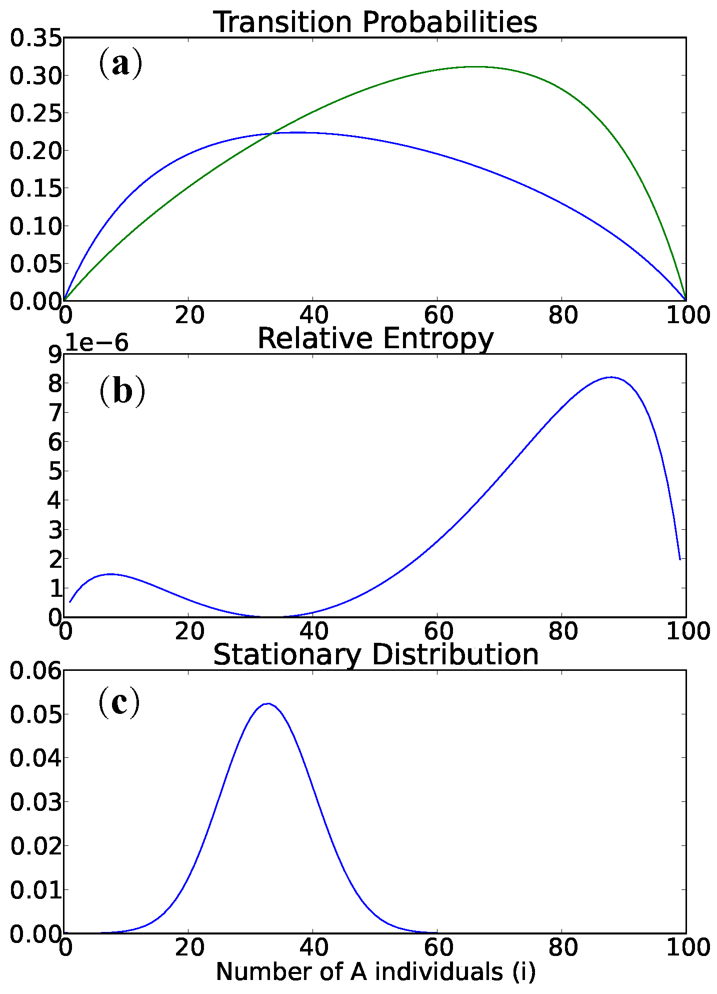
2.1. Main Theorem for Two-Type Incentive Processes
First we show that when the stationary distribution is locally maximal or minimal, the distance between
and
is minimal. We require a technical lemma to prove the main theorem that concerns continuity of incentive-proportionate replication probabilities. The crux of the proof is essentially that from the stationary distribution we have that if
is local maximum or minimum of the stationary distribution then
Note there are two directions for the path through the states in Equation (
4), ending with
or
, so there is a second solution to the ISS max/min criteria as well. To satisfy
we need
So we need “equality” of the right-hand sides to ensure that these criterion are both satisfied, and we can argue that this is the case for sufficiently large N by appealing to continuity. This should not be surprising—in both cases, the population is shifting by one in the same direction, and as N gets larger, these points are closer together since for large N.
Lemma 1. Suppose the vector of incentive proportionate selection probabilities p as defined in Equation (
1)
is a continuous function of and let .
Then for the incentive process defined in Equation (
2),
there exists an integer such that for we have that Proof. Since p is a continuous function of , so is . Let and . For we simply need to choose N large enough so that the set of population states is sufficiently fine-grained enough so that . Continuous functions on compact spaces (the simplex) are uniformly continuous, so continuous implies there is such that if then for all a and b. Since , is sufficient. ☐
If the incentive function is continuous as a function of , and the mutations are constant or otherwise continuous as functions of a, then we have that is also continuous, satisfying the hypothesis of the lemma.
Theorem 1. For a continuous incentive and mutation matrix, there is a sufficiently large N so that local maxima and minima of the stationary distribution of the incentive process are local minima of the distance for ; interior extrema are local minima of the relative entropy .
Proof. If
is a maximum or minimum of the stationary distribution then by the formula for the stationary distribution (Equation (
4)) we must have that the last term in the product passes through 1 so that the stationary distribution switches from increasing to decreasing (or vice versa). By continuity there is
where the ratio is exactly equal to one by the intermediate value theorem, and so the state
satisfies
. Note that
i and
j are not necessarily equal, and
j may not be an integer (not a true state of the process). This is the difference between being a local extremum of the stationary distribution on a partition of the simplex and being a local extremum of the associated continuous function on the simplex. To complete the proof we will assume that
N is sufficiently large enough that the states corresponding to
i and
j are close so that we can assume that
(by continuity).
Let
. Then by the lemma and the triangle inequality, for sufficiently large
N, we have that:
For the
-distance, we have that, by Proposition 2 (at interior states):
and similarly at boundary states for
,
. This shows that
vanishes for large
N at the extremum. For neighboring states, the divergence between the state and the expected next state does not vanish: if this were the case, the transition probabilities between the adjacent states would be equal, and the stationary probabilities equal, contradicting the assumption of a local stationary extremum. Therefore
is locally minimal. ☐
A maximum of the stationary distribution need not occur when is maximal, hence it is not a good definition of stability. The converse of the theorem is not true; the Lyapunov quantity may be minimized but fail to have a local maximum or minimum of the stationary distribution. While we have only proven that the theorem for large N for arbitrary continuous incentives, it may be possible to make sharper estimates based on the form of the incentive. As we will see from the examples for dimensions greater than 2, for linear landscapes the theorem seems to hold for almost any N with few exceptions.
For the replicator equation, it is known that there is at most one asymptotically stable interior state for linear fitness landscapes. We have a similar result in this context as a corollary.
Corollary 1. For two-type populations and linear fitness landscapes with the Moran process, if as then there is at most one interior stationary stable state as .
Note that the hypothesis that is necessary, otherwise one can find counterexamples with multiple interior stationary maximum for specific parameters, e.g., , and game matrix given by , produces a process with interior local maxima at . In fact for this game, any produces two interior solutions, , so long as N is large enough for the solutions to be more than from the boundaries. (Note that Theorem 1 still holds.)
2.2. k-Fold Incentive Process
These two propositions show that the main theorem for locally-balanced birth-death processes will apply to the k-fold incentive process for all k.
Proposition 4. The stationary distribution of a Markov process X is the same as the stationary distribution of the process , defined by the k-th power of the transition matrix.
Proof. The stationary distribution of a Markov chain can be obtained by the rows of the matrix defined by
and so the stationary distributions of the
k-fold incentive process are the same for all
k, given a fixed transition matrix
T. ☐
The next proposition follows easily from the fact that the k-fold incentive process has the same stationary distribution and the definition of matrix multiplication.
Proposition 5. If a Markov process X satisfies the detailed-balance condition, so does the process defined by the k-th power of the transition matrix.
Corollary 2. Theorem 1 holds for the k-fold incentive process for two-type populations.
Examples
As an illustration of how large
N may need to be, we consider the
q-replicator incentive and game matrix defined by
,
. Direct substitution shows that
is a solution to the ISS candidate equation for all
q and
μ. (Note that for
,
and
are also solutions.) For the two stationary extrema equations, we have that
. For large
N, these solutions all converge to
. Even for small
N, these solutions differ only by a small amount (
). Similarly, for the landscape given by
,
, we can give an explicit formula for the stationary distribution for arbitrary
μ (see [
35]):
Since only the binomial factor depends on j, it is clear that is the local maximum of the stationary distribution for any μ and any . So we see explicitly that the property of being stationary stable is dependent on the population size N.
Let the fitness landscape be defined by the
q-replicator incentive and the game matrix
,
(the Moran landscape with relative fitness
) and let
for
. As shown in [
24], for
there is an internal candidate ISS. We consider three cases. For
, there is no ISS (the transition probabilities never intersect), and no internal local maximum of the stationary distribution. The latter is true for
as well, but there is a state where the transitions intersect, and
is locally minimal at this state (
), which shows that a candidate ISS need not be stable in the sense of the stationary distribution. An imbalanced mutation rate can force an internal equilibrium for
, for instance with
and
. For
, the projection incentive, there is a local maximum of the stationary distribution (at
). It is unique and
is minimal.
It is possible to have multiple interior stationary stable states for the replicator incentive with . For example, the following parameters give a process with two local maxima of the stationary distribution: , , , and the neutral fitness defined by . It is also possible to have an internal local stationary maximum as well as a boundary maximum, e.g., for , , , , fitness landscape defined by , , , .
2.3. Main Theorem for Globally Balanced Incentive Processes
In general, incentive processes for more than two-types need not be locally-balanced, so we cannot use Equation (
4) to establish the main theorem. In fact, it appears to rarely be the case (the neutral landscape is an exception in some cases), though computations indicate that in some cases, the detailed balance condition is nearly satisfied, and Equation (
4) produces a good approximation of the stationary distribution. Regardless, we now generalize Theorem 1 to globally-balanced incentive processes. The proof strategy is similar to the locally-balanced case, using the global balance equation instead.
Any probability inflow-outflow balanced state, i.e., any state such that , will minimize the distance between the expected next state and the current state. We will call such states probability flow neutral. This could happen in principle at, e.g., a saddle point, but since we are mostly concerned with stationary maxima for stability purposes, we will focus on maxima.
Proposition 6. For a continuous incentive and mutation matrix and sufficiently large N, local maxima and minima of the stationary distribution are probability flow neutral. Precisely, for ,
there is an such that for ,
Proof. We prove just the maximal case. Suppose we have local maxima
a of the stationary distribution and let
. Since all the transition probabilities are continuous in the population state, so is the stationary distribution, which is therefore uniformly continuous and bounded by
M. For sufficiently large
N we can choose
ϵ so that
for states
b adjacent to
a. By the global balance equation,
so dividing through by
and using the above inequality for
,
☐
We take it as given that stationary extrema occur at probability flow neutral states, knowing that the population states may differ by a small amount. Now we show that stationary extrema minimize the distance functions . While the relative entropy is only well-defined on the interior of the simplex, the same result holds when the state space is restricted to a boundary simplex of lower dimension. This means that the relative entropy can still detect boundary stable points of the same process on the restricted subspace, but the other do so on the full simplex.
Theorem 2. For a continuous incentive and mutation matrix on n types, there is a sufficiently large N so that probability flow neutral states of the incentive process are local minima of the distance functions for ; interior extrema are local minima of the relative entropy .
Proof. Since the proof is similar to the two-type case, we just sketch the proof. Let
and suppose that
a is a probability flow neutral state of the process:
We have that
, and we use continuity to choose a sufficiently large
N so to replace right-hand terms with
(as in the lemma before Theorem 1). Then we have that
☐
Since the k-fold incentive process has the same stationary distribution as the case, and since the expected value functions agree at equilibrium via Proposition 1, we have the next theorem as an immediate corollary. This shows in particular that the connection between the stationary distribution and evolutionarily stable states can hold for generational processes.
Theorem 3. Theorem 2 holds for the k-fold incentive process.
2.4. Three Type Examples
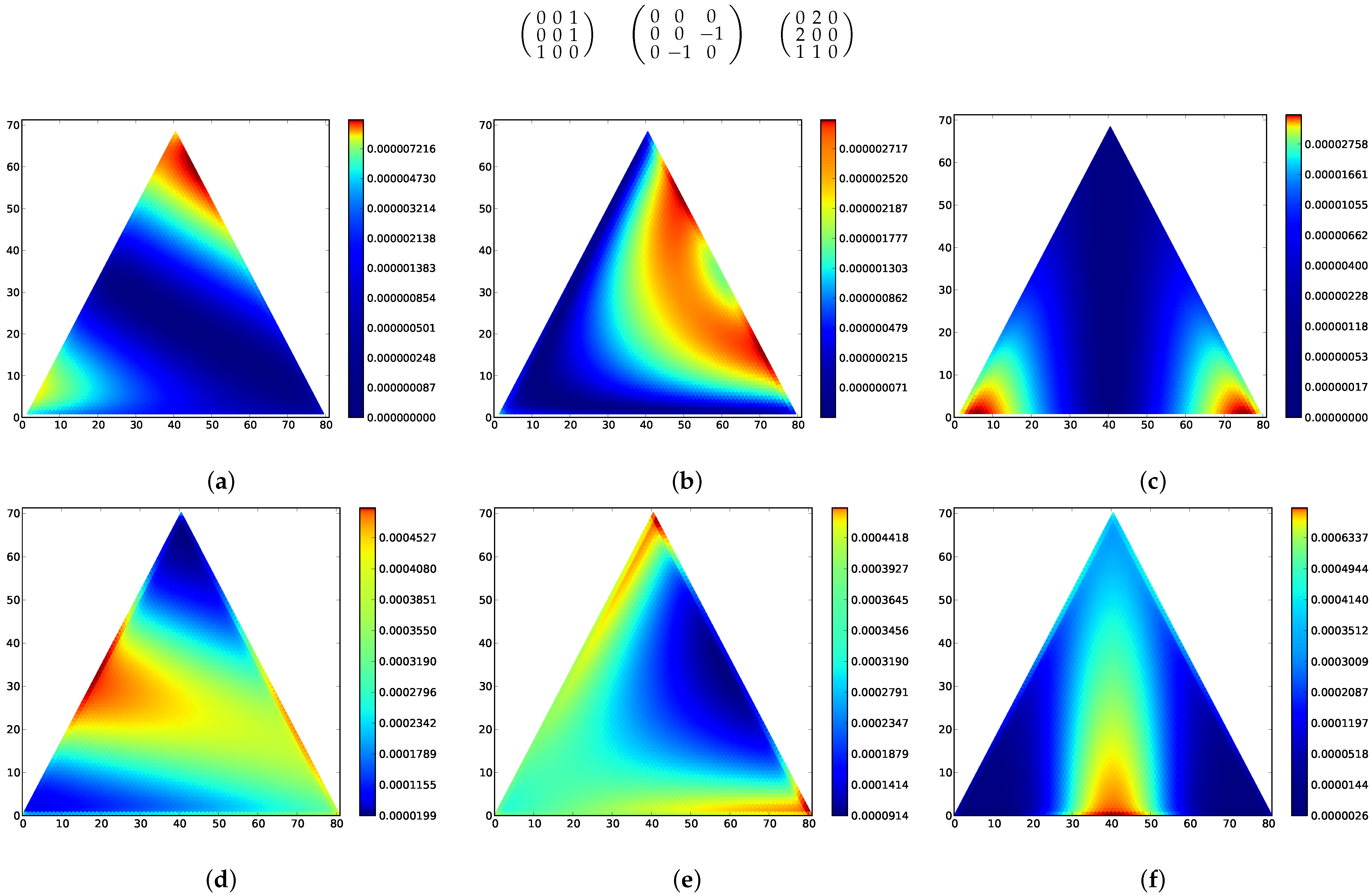
Here we give several interesting examples using Bomze’s classification of three-type phase portraits for the replicator dynamic with linear fitness landscape (see [
58] and the additions and corrections [
59]). We use the Fermi incentive for all examples. A full list corresponding to each of the 48 phase portraits is available online at
http://marcharper.net/stationary_examples/index.html.
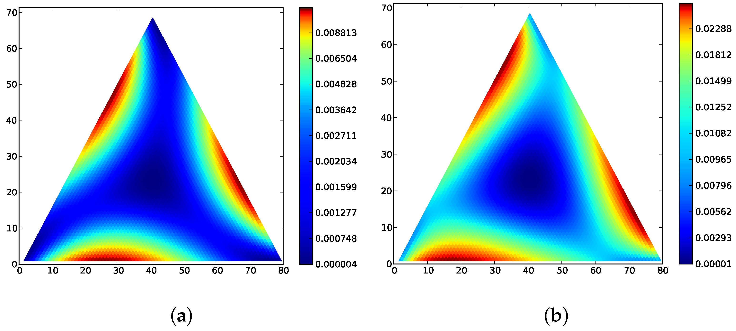
Figure 2 gives stationary distributions and expected distances for the following game matrices, to illustrate Theorem 2.
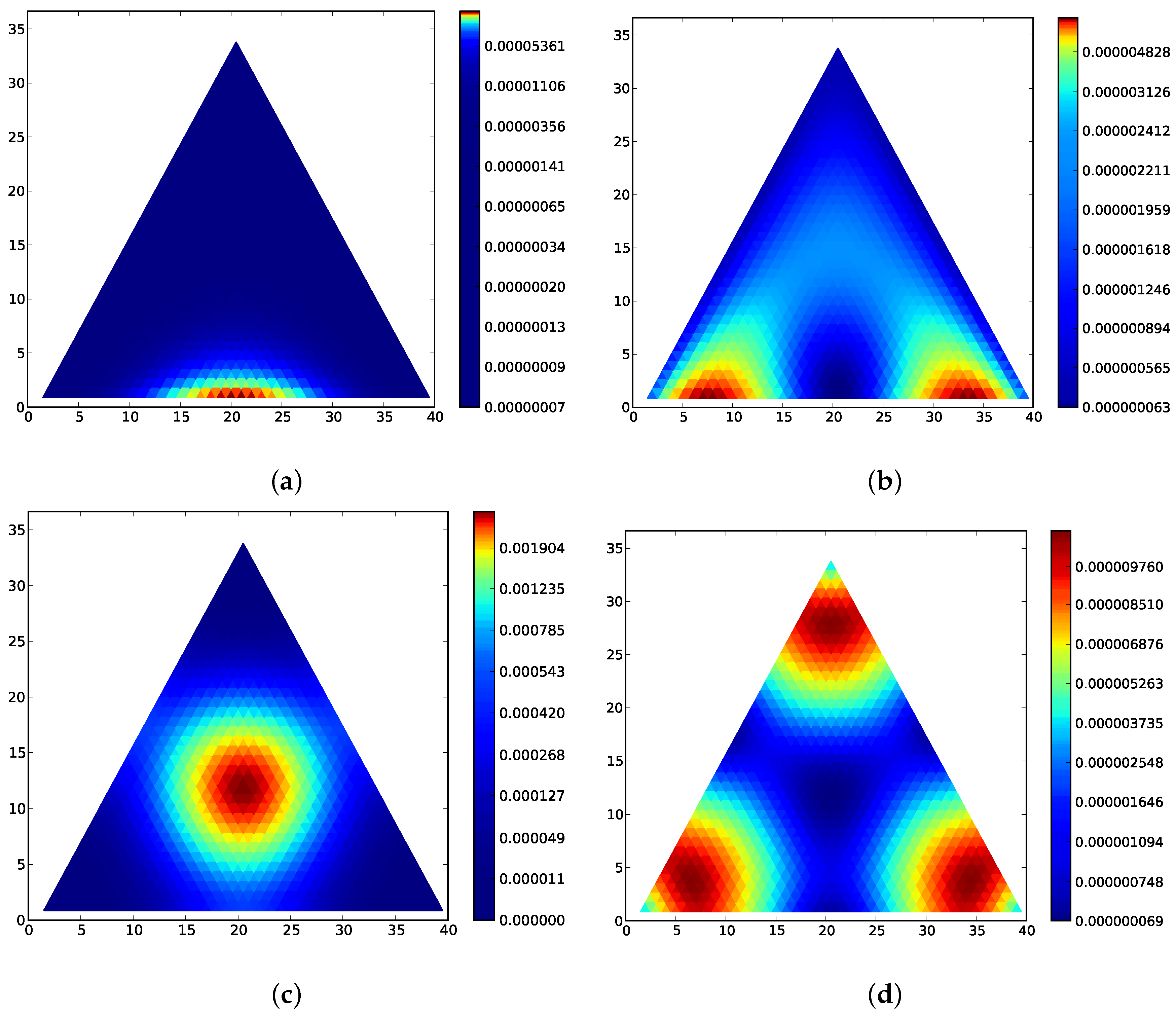
2.5. Rock-Scissors-Paper Games
The rock-scissors-paper game is given by a matrix of the form:
In [
42] (online supplement), Andrae et al. give steady-state distributions for the rock-scissors-paper game in the context of entropy production.
Figure 3 contains stationary distributions for the rock-scissors-paper game; these are qualitatively similar to those in
Figure 4 of [
42]. Traulsen et al. consider the average drift of a relative entropy equivalent Lyapunov quantity in [
25] for the Moran process in a finite population, and find that convergence depends on the value of
N. The rock-scissor-paper game for the Moran process does not yield a detail-balanced Markov process [
42], and because of the cyclic-nature of the process, the transitions are particularly removed from detailed-balance. This is reflected in the fact that the stationary distribution can take many iterations of the transition matrix to converge. These plots also illustrate that the stability of particular states depends significantly on the mutation rate.
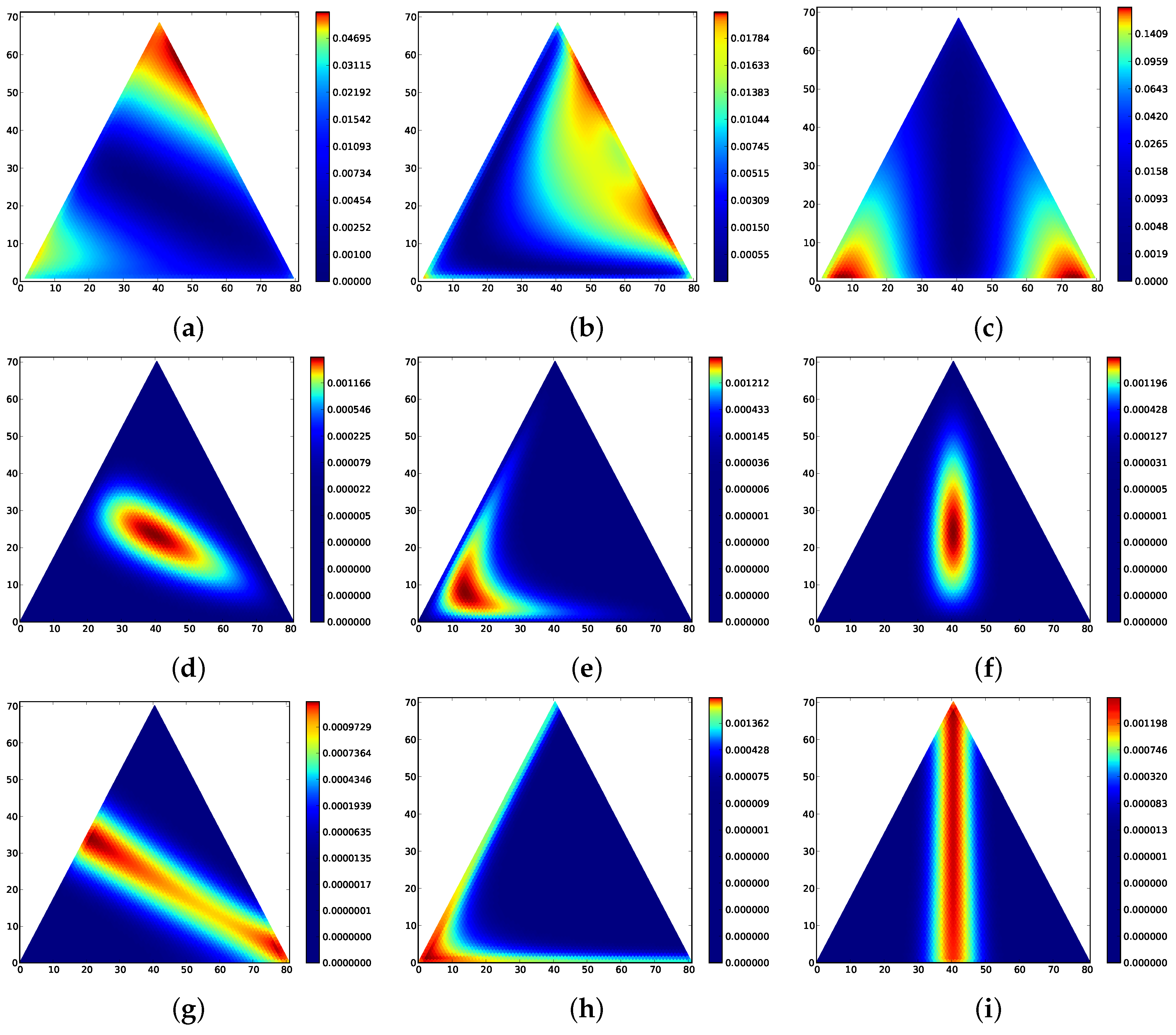
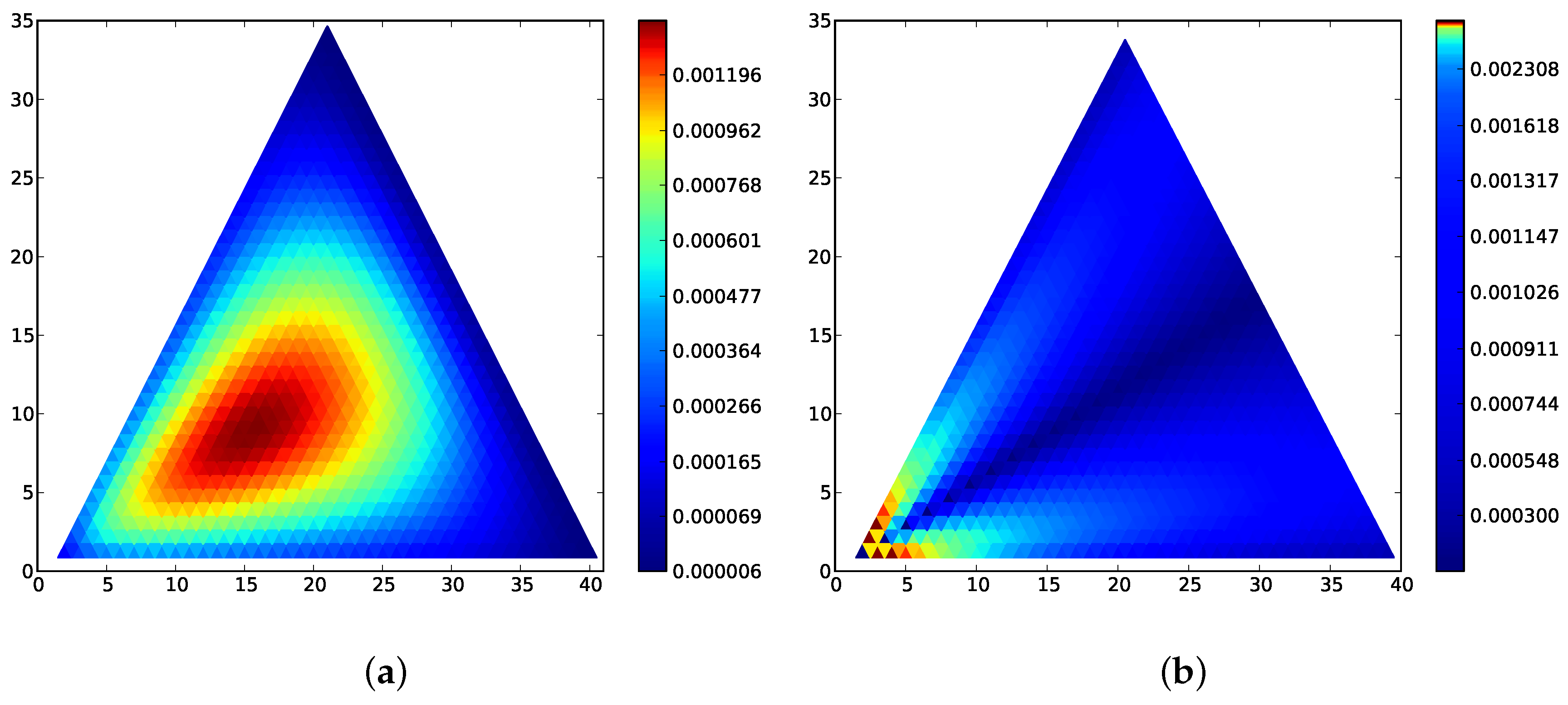
2.6. Four Types
For completeness, we include a higher dimensional example. Consider the incentive process defined by the Fermi incentive,
,
and the game matrix
Although we cannot easily plot the full stationary distribution, we can plot the two-dimensional boundary simplices.
Figure 5 gives the
expectation distance and the stationary distribution for two of the four faces. Three are the same; the fourth, where
, is distinct, and similar to the stationary distribution in
Figure 1. From inspection of the game matrix, we would predict that
is an ISS for the distinct face. The three similar faces have boundary ISS such as
. Note that the stationary distribution and
expected distances are computed for the full process on the three-dimensional state space; only the two-dimensional faces are plotted.
2.7. The Wright–Fisher Process
The Wright–Fisher process behaves differently than the Moran process for many combinations of parameters; see, e.g., [
18]. In general, even for two-types, the Wright–Fisher process is not locally balanced [
19]. Because of the combinatorial complexity of the process, the Wright–Fisher process is often studied via diffusion-type approximations. In some cases, these differential equations produce a qualitatively similar result to our main theorem for the incentive process. For instance in [
60], the authors show that for the replicator incentive, the limiting distribution of the diffusion approximation concentrates on ESS. Combined with the fact that
is the same as for the incentive process (Proposition 1), one can reasonably expect some subset of the parameters to produce a similar result to Theorem 1 for the Wright–Fisher process. See
Figure 2 for examples.
We give an partial analog of Theorem 1 for the Wright–Fisher process. Crucially, note that a local maximum of the stationary distribution of the Wright–Fisher process is in fact a global maximum since every state is connected directly to every other state (assuming that that transition probabilities are never zero), and therefore is necessarily unique.
Theorem 4. Suppose a given incentive and mutation matrix are continuous. For the Wright–Fisher process, suppose that the stationary distribution has a global maximum at a, is symmetric about the maximum, and is otherwise vanishingly small (if the maximum is not central). Then for sufficiently large N, the state a is an ISS candidate and a minimum of the distance .
Proof. We only give the case for
in detail. Since the stationary distribution satisfies
, we have that
where
denotes an adjacent state and by continuity for some
j we must have that
(at the maximum since the distribution is symmetric). A bit of algebra shows that this occurs when
For sufficiently large N, solutions to this equation are the same as those of the ISS candidate equation. For , looking at all the immediately adjacent states leads to for large N, which implies by summation that . ☐
Computationally, we can compute the stationary distribution of the Wright–Fisher process for any combination of parameters for smaller
easily.
Figure 2 and
Figure 6 give a variety of computational examples, some of which suggest that a more general version of Theorem 4 holds. Note the sensitivity to the mutation rate
μ. Qualitatively,
Figure 1 is similar for the Wright–Fisher process on the interior. Figures for all 48 of the landscape in Bomze’s classification are also available online at
http://people.mbi.ucla.edu/marcharper/stationary_stable/3x3/.


