
Indicators of Evidence for Bioequivalence

Abstract
:
1. Introduction
1.1. Background and Summary
1.2. Properties of Evidence in One-Sided Z-Tests
1.3. Properties of Evidence in Two One-Sided Z-Tests (TOST)
1.3.1. How Evidence Grows with Sample Size in Two One-Sided Z-Tests
1.3.2. Sample Size Determination
1.4. Connection of Evidence in TOST with a One-Sided Test
2. More Examples of Two One-Sided Tests (TOSTS)
2.1. Evidence for Equivalence in Two One-Sided Binomial Tests
2.2. Evidence for Equivalence of Risks
2.3. Evidence for Equivalence in Two One-Sided t-Tests
Approximate Normality of the Variance Stabilized t-Statistic
3. Evidence in Multivariate Equivalence Tests
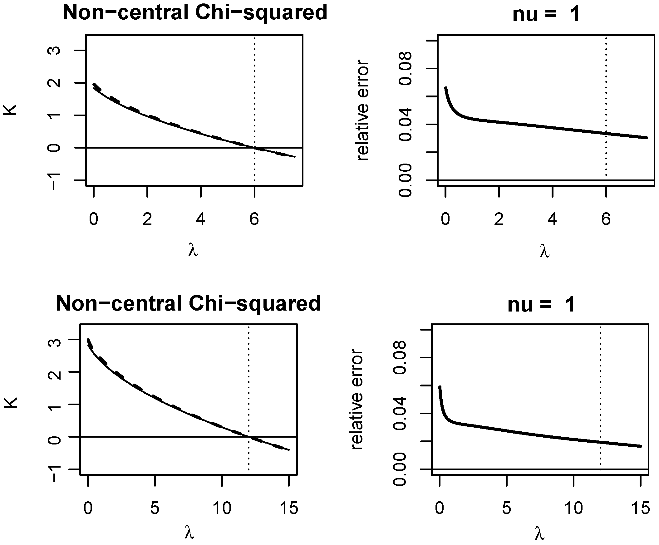
3.1. A VST for the Non-Central Chi-Squared Statistic
3.2. Evidence for Equal Means
3.3. Application to between Group Sum of Squares
4. Testing for Equivalence of K Groups
5. Summary and Discussion
Acknowledgments
Author Contributions
Conflicts of Interest
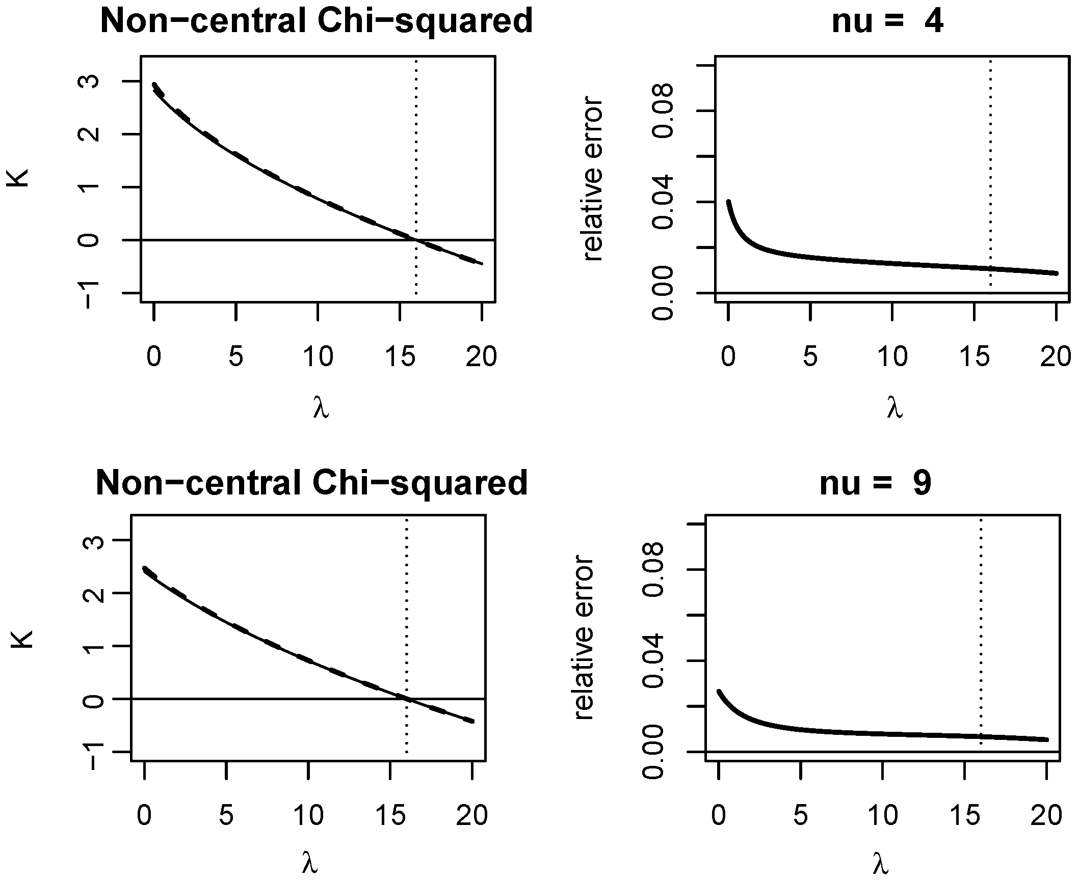
Appendix A. Quality of KLD Approximations
Appendix A.1. Non-Central Chi-Squared Distribution

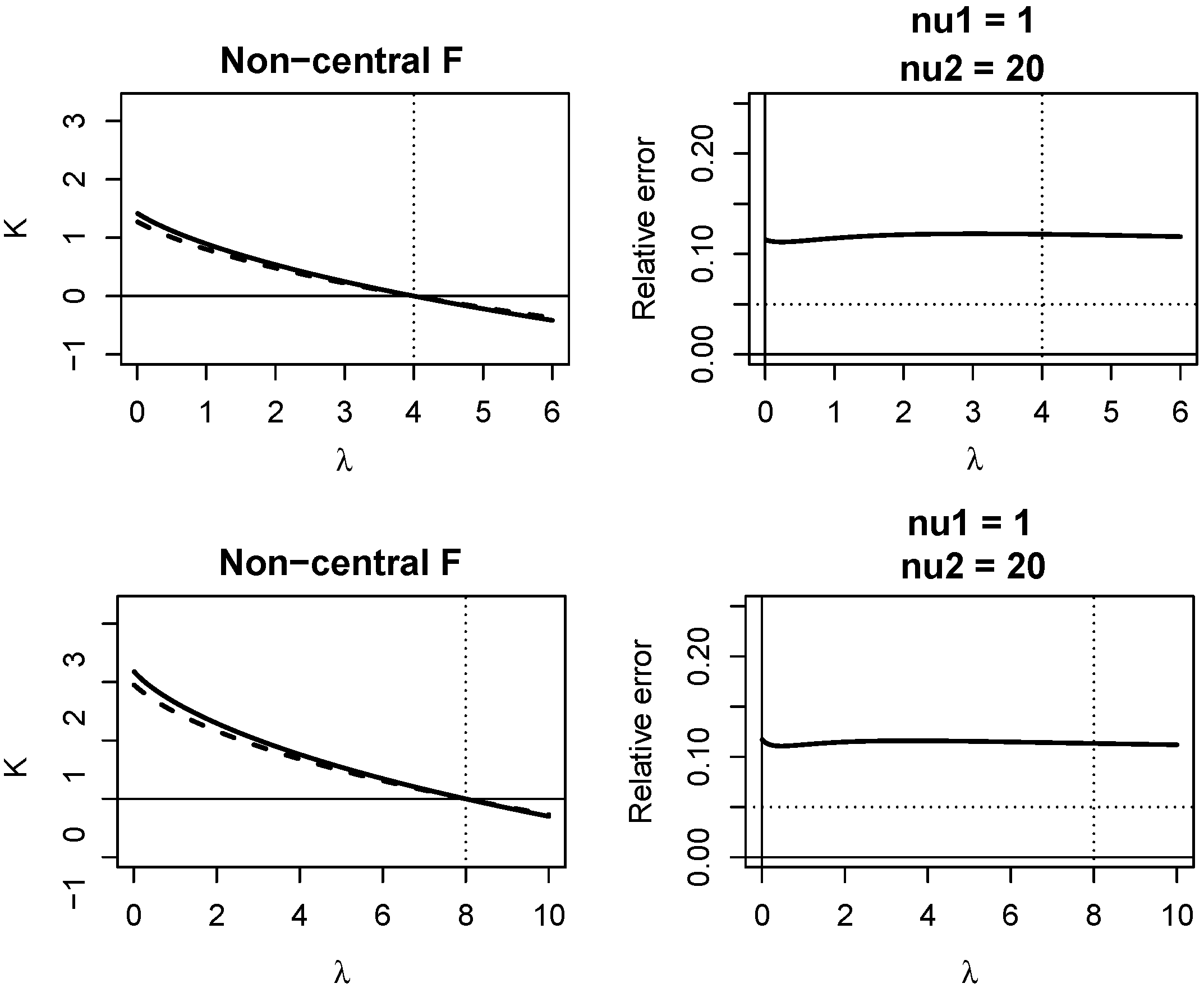
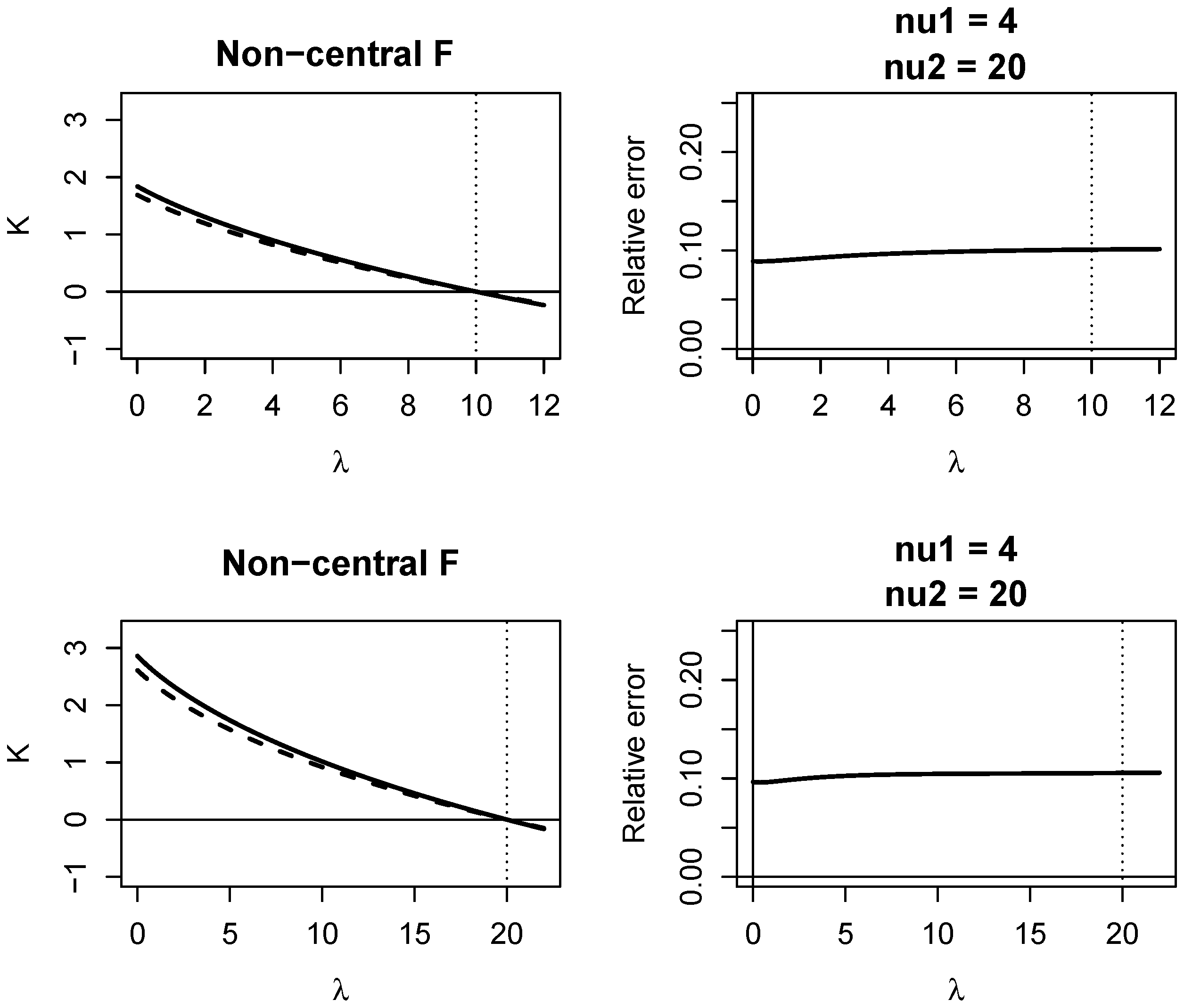
Appendix A.2. Non-Central F Distribution


Appendix B. R Scripts for Computing VSTs
#############  Evidence for equivalence
#############  using TOST, and one-sample binomial data
vstbinom <_ function(n,p)
{h <_ 2*sqrt(n)*asin(sqrt(p))
return(h)}

############# Usually p1=p0-Delta0,p2=p0+Delta0
bioevid <_ function(n,p1,p2,phat)
{Tminus <_  vstbinom(n,phat)-vstbinom(n,p1)
Tplus  <_  vstbinom(n,p2)-vstbinom(n,phat)
evidforequiv <_ min(Tminus,Tplus)
out <_ c(Tminus,Tplus,evidforequiv)
outrd <_ round(out,digits=3)
return(outrd)}

#############  Example 1 of the text. (data from Example 4.2 of Weller, page 59.)
n <_ 273
phat <_ 199/273
p1 <_ 0.65
p2 <_ 0.75
bioevid(n,p1,p2,phat)

############################################################################
############# Evidence for equivalence for risk difference

vstRD <_ function(n1,p1hat,n2,p2hat,Delta0)
{Deltahat <_ p1hat-p2hat
pbarhat <_ (p1hat+p2hat)/2
N <_ n1+n2
vhat <_ (1-2*pbarhat)*(1/2-n2/N)
what <_ sqrt(pbarhat*(1-pbarhat)+vhat^2)
vst <_ sqrt(4*n1*n2/N)*(asin((Deltahat/2 +vhat)/what)-asin((Delta0/2 +vhat)/what))
return(vst)}

############## Usually Delta1= -Delta0 and Delta2= +Delta0
bioevidRD <_ function(x1,n1,x2,n2, Delta1,Delta2)
{p1hat <_ (x1+0.5)/(n1+1)
p2hat <_ (x2+0.5)/(n2+1)
Deltahat <_ p1hat-p2hat
Tminus <_  vstRD(n1,p1hat,n2,p2hat,Delta1)
Tplus  <_  -vstRD(n1,p1hat,n2,p2hat,Delta2)
T <_ min(Tminus,Tplus)
out <_ c(Deltahat,Tminus,Tplus,T)
outrd <_ round(out,digits=3)
return(outrd)}

####### Example 2 of the text. (data from Dunnett and Gent(1977) Biometrics)
x1 <_ 148
n1 <_ 225
x2 <_ 115
n2 <_ 167
Delta1 <_ -0.1
Delta2 <_ 0.1
bioevidRD(x1,n1,x2,n2, Delta1,Delta2)

###########################################################################
## Linear extension of vst for chisq(nu,lambda) (Equation (13) of the text.)

evidchisqlin <_ function(s,nu,lambda0,M)
{smalls <_ s[s <= nu]
Tsmall <_ M-sqrt(s[s>nu]-nu/2)  ## usual vst
grad <_ -sqrt(nu/2)/nu
Tbig <_ M +grad*s[s<=nu]
T <_  c(Tbig,Tsmall)
return(T)}

Mfun <_ function(nu,lambda0)    ## requires lambda0 > nu/2
{return(sqrt(lambda0))}

# Mfun2 <_ function(nu,lambda0) ##  The user may want to supply their own M.
# {return(sqrt(lambda0+nu)-sqrt(nu/10))}

############### Plot evidence function (illustrative example)
nu = 3
lambda0 = 6
maxexev <_ sqrt(lambda0+nu/2)-sqrt(nu/2)
maxexev
M <_ Mfun(nu,lambda0)
M
s <_ c(seq(0,lambda0+nu,.01))
T <_  evidchisqlin(s,nu,lambda0,M)
plot(s,T,type="l",lwd=2,main="Evidence for equivalence")
abline(h=maxexev,lty=3)
abline(h=0)

##################### To examine properties of evidence function.
lambda = lambda0   ## Try this and other lambda, where 0 <= lambda < lambda0.
s <_ rchisq(10000,nu,lambda)
T <_ evidchisqlin(s,nu,lambda0,M)
mean(T)
sd(T)
hist(T)

###########################################################################
## Linear extension of VST for F(nu1,nu2,lambda) (Equation (19) of the text.)

evidFlin <_ function(s,nu1,nu2,lambda0,M)   ### nu2>4
{c <_ (nu2/nu1)*sqrt((nu1+nu2-2)/(nu2-2))
b <_ nu2/(nu2-2)
a <_ sqrt((nu2-4)/2)
Tsmall <_  M-a*acosh((s[s>b]+nu2/nu1)/c)
grad <_ -a*acosh((b+nu2/nu1)/c)/b
Tbig <_ M+grad*s[s<=b]
T <_  c(Tbig,Tsmall)
return(T)}

###################    Example 5 of the text. (data from Wellek, Example 7.2, p.165.)

n1 <_ 10
x1bar <_ 99.8120
s1 <_ 7.5639
n2 <_ 12
x2bar <_ 99.2903
s2 <_ 5.9968
n3 <_ 13
x3bar <_ 100.0024
s3 <_ 10.4809
n4 <_ 15
x4bar <_ 98.6407
s4 <_ 4.5309
N <_ n1+n2+n3+n4  ##
xbarbar <_ (n1*x1bar+n2*x2bar+n3*x3bar+n4*x4bar)/N  ## 99.3849
K <_ 4
nbar <_ N/K
ssqW <_ (n1-1)*s1^2+(n2-1)*s2^2+(n3-1)*s3^2+(n4-1)*s4^2
ssqB <_ n1*(x1bar-xbarbar)^2+n2*(x2bar-xbarbar)^2+n3*(x3bar-xbarbar)^2
ssqB <_ ssqB+n4*(x4bar-xbarbar)^2

epsilon <_ 1/2                 ## Wellek’s choice
nu1 <_ K-1
nu2 <_ N-K
lambda0 <_ 12.5*0.25*1.35      ## nbar*eps^2*vu*bnu = 4.21875

nu1 <_ K-1
nu2 <_ N-K

epsilon <_ 1/2                 ## this is arbitrary; want max_k |mu_k-mu|/sigma < epsilon
lambda0 <_ 12.5*0.25*1.35      ## nbar*eps^2*vu1*bnu1 = 4.21875

MFfun <_ function(nu1,nu2,lambda0)
{return(sqrt(lambda0+nu1/(nu1+nu2)))}

M <_ MFfun(nu1,nu2,lambda0)
S <_   (ssqB/nu1)/(ssqW/nu2)     ## 0.0926 (Value of F-statoistic.)

evidFlin(S,nu1,nu2,lambda0,M)    ## T = 1.934

################  To compute maximum expected evidence, require:

exS <_ function(lambda,nu1,nu2)   ##### this computes expected value of S
{return(nu2*(n1+lambda)/(nu1*(nu2-2)))}

c <_ (nu2/nu1)*sqrt((nu1+nu2-2)/(nu2-2))
b <_ nu2/(nu2-2)
a <_ sqrt((nu2-4)/2)
M <_ sqrt(lambda0-nu1/(nu1+nu2))
M
maxexev <_ -a*acosh((exS(0,nu1,nu2)+nu2/nu1)/c)+
a*acosh((exS(lambda0,nu1,nu2)+nu2/nu1)/c)

maxexev

############### Plot evidence function (illustrative example)

s <_ c(seq(0,exS(lambda0,nu1,nu2)+1,.01))
T <_  evidFlin(s,nu1,nu2,lambda0,M)
plot(s,T,type="l",lwd=2,ylim=c(-1,M),main="Evidence for equivalence")
abline(h=maxexev,lty=3)
abline(h=0)
abline(v=lambda0,lty=3)

################################# To examine properties of evidence function
lambda=0 ## Try this and other lambda, where 0 <= lambda < lambda0.lambda = lambda0

s <_ rf(10000,nu1,nu2,lambda)
T <_  evidFlin(s,nu1,nu2,lambda0,M)
mean(T)
sd(T)
hist(T)
References
- Schuirmann, D.J. A comparison of two one-sided tests procedure and the power approach for assessing the equivalence of average bioavailability. J. Pharm. Biopharm. 1987, 15, 657–680. [Google Scholar] [CrossRef]
- Berger, R.; Hsu, J.C. Bioequivalence trials, intersection-union tests and equivalence confidence sets with discussion. Stat. Sci. 1996, 11, 283–302. [Google Scholar]
- Senn, S. Statistical issues in equivalence testing. Stat. Med. 2001, 20, 2785–2799. [Google Scholar] [CrossRef] [PubMed]
- Dragalin, V.; Fedorov, V.; Patterson, S.; Jones, B. Kullback–leibler divergence for evaluating bioequivalence. Stat. Med. 2003, 22, 913–930. [Google Scholar] [CrossRef] [PubMed]
- Lauretto, M.; Pereira, C.A.B.; Stern, J.M.; Zacks, S. Full Bayesian Signicance Test Applied to Multivariate Normal Structure Models. Braz. J. Probab. Stat. 2003, 17, 147–168. [Google Scholar]
- Chervoneva, I.; Hyslop, T.; Hauck, W.W. A multivariate test for population bioequivalence. Stat. Med. 2007, 26, 1208–1223. [Google Scholar] [CrossRef] [PubMed]
- Ocaña, J.; Sanchez, M.P.; Sanchez, A.; Carrasco, J.L. On equivalence and bioequivalence testing. Sort 2008, 32, 151–158. [Google Scholar]
- Tsai, C.A.; Huang, C.Y.; Liu, J.P. An approximate approach to sample size determination in bioequivalence testing with multiple pharmacokinetic responses. Stat. Med. 2014, 33, 3300–3317. [Google Scholar] [CrossRef] [PubMed]
- Kulinskaya, E.; Morgenthaler, S.; Staudte, R.G. Meta Analysis: A Guide to Calibrating and Combining Statistical Evidence; John Wiley & Sons: Hoboken, NJ, USA, 2008. [Google Scholar]
- Morgenthaler, S.; Staudte, R.G. Advantages of variance stabilization. Scand. J. Stat. 2012, 39, 714–728. [Google Scholar] [CrossRef]
- Kulinskaya, E.; Morgenthaler, S.; Staudte, R.G. Variance stabilizing the difference of two binomial proportions. Am. Stat. 2010, 64, 350–356. [Google Scholar] [CrossRef]
- Morgenthaler, S.; Staudte, R.G. Evidence for alternative hypotheses. In Robustness and Complex Data Structures; Becker, C., Fried, R., Kuhnt, S., Eds.; Springer: Berlin/Heidelberg, Germany, 2013; pp. 315–329. [Google Scholar]
- Prendergast, L.A.; Staudte, R.G. Better than you think: Interval estimators of the difference of binomial proportions. J. Stat. Plan. Inference 2014, 148, 38–48. [Google Scholar] [CrossRef]
- Johnson, N.L.; Kotz, S.; Balakrishnan, N. Continuous Univariate Distributions, 2nd ed.; Wiley: New York, NY, USA, 1994; Volume 1. [Google Scholar]
- Johnson, N.L.; Kotz, S.; Balakrishnan, N. Continuous Univariate Distributions, 2nd ed.; Wiley: New York, NY, USA, 1995; Volume 2. [Google Scholar]
- Leone, F.C.; Nelson, L.S.; Nottingham, R.B. The folded normal distribution. Technometrics 1961, 3, 543–550. [Google Scholar] [CrossRef]
- Wellek, S. Testing Statistical Hypotheses of Equivalence; CRC Press: Boca Raton, FL, USA, 2003. [Google Scholar]
- Dunnett, C.W.; Gent, M. Significance testing to establish equivalence between treatments, with special reference to data in the form of 2 × 2 tables. Biometrics 1977, 33, 593–602. [Google Scholar] [CrossRef] [PubMed]
- Johnson, R.; Dunnett, C.W.; Gent, M. p-values in 2 × 2 tables. Biometrics 1988, 44, 907–910. [Google Scholar]
- Wellek, S. Testing Statistical Hypotheses of Equivalence and Noninferiority, 2nd ed.; CRC Press: Boca Raton, FL, USA, 2014. [Google Scholar]
- Laubscher, N.F. Normalizing the noncentral t and f distributions. Ann. Math. Stat. 1960, 31, 1105–1112. [Google Scholar] [CrossRef]
- Kullback, S. Information Theory and Statistics; Dover: Mineola, NY, USA, 1968. [Google Scholar]


| t | 0 | 1.281 | 1.645 | 2.326 | 3.090 | 3.3 | 3.719 | 5 |
| p-value | 0.5 | 0.10 | 0.05 | 0.01 | 0.001 | 0.0005 | 0.0001 | 0.0000003 |
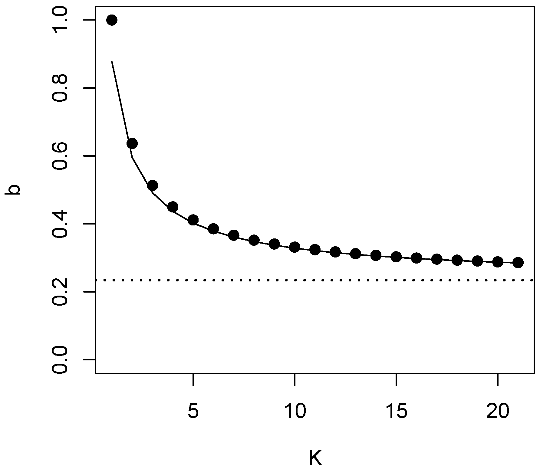
| K | 2 | 3 | 4 | 5 | 6 | 7 | 8 | 10 | 50 | 100 | ∞ |
|---|---|---|---|---|---|---|---|---|---|---|---|
| 0.513 | 0.450 | 0.412 | 0.386 | 0.367 | 0.352 | 0.332 | 0.259 | 0.248 | 0.23420... | ||
| 0.595 | 0.492 | 0.437 | 0.402 | 0.379 | 0.361 | 0.348 | 0.329 | 0.259 | 0.248 |
© 2016 by the authors; licensee MDPI, Basel, Switzerland. This article is an open access article distributed under the terms and conditions of the Creative Commons Attribution (CC-BY) license (http://creativecommons.org/licenses/by/4.0/).
Share and Cite
Morgenthaler, S.; Staudte, R. Indicators of Evidence for Bioequivalence. Entropy 2016, 18, 291. https://doi.org/10.3390/e18080291
Morgenthaler S, Staudte R. Indicators of Evidence for Bioequivalence. Entropy. 2016; 18(8):291. https://doi.org/10.3390/e18080291
Chicago/Turabian StyleMorgenthaler, Stephan, and Robert Staudte. 2016. "Indicators of Evidence for Bioequivalence" Entropy 18, no. 8: 291. https://doi.org/10.3390/e18080291
APA StyleMorgenthaler, S., & Staudte, R. (2016). Indicators of Evidence for Bioequivalence. Entropy, 18(8), 291. https://doi.org/10.3390/e18080291