Entropy Generation on MHD Eyring–Powell Nanofluid through a Permeable Stretching Surface

Abstract

In this article, entropy generation of an Eyring–Powell nanofluid through a permeable stretching surface has been investigated. The impact of magnetohydrodynamics (MHD) and nonlinear thermal radiation are also taken into account. The governing flow problem is modeled with the help of similarity transformation variables. The resulting nonlinear ordinary differential equations are solved numerically with the combination of the Successive linearization method and Chebyshev spectral collocation method. The impact of all the emerging parameters such as Hartmann number, Prandtl number, radiation parameter, Lewis number, thermophoresis parameter, Brownian motion parameter, Reynolds number, fluid parameter, and Brinkmann number are discussed with the help of graphs and tables. It is observed that the influence of the magnetic field opposes the flow. Moreover, entropy generation profile behaves as an increasing function of all the physical parameters.

1. Introduction

In recent years, nanofluid has received more and more attention by various scientists due to its numerous applications in engineering and various industrial processes. A nanofluid is comprised of a base fluid with tiny (nanometer) sized nanoparticles, such as carbides or carbon nanotubes, oxides, and metals, whereas traditional base liquids involve ethylene glycol, oil, and water. A nanofluid is very helpful in enhancing thermal conductivity and convection of heat transfer coefficient when it is analyzed with the base fluid. In modern technology, nanomaterials are becoming increasingly important in the performance of various heat exchangers, such as microelectronics, optical modulators, and chemical production. Magneto-nanofluids are also remarkable for their use in various applications, such as tunable optical fiber filters, magneto-optical wavelength filters, optical modulators, and optical switches. In biomedical engineering, magneto-nanoparticles are also very helpful in cancer therapy, sink-float separation, hyperthermia, magnetic resonance imaging (MRI), magnetic cell separation, drug delivery, and magnetic drug targeting. In particular, heat transfer and convective flow are influenced by the features of nanofluids, such as thermal conductivity and viscosity. Conventional heat transfer in various Newtonian and non-Newtonian fluids, such as ethylene glycol, oil, water, etc., holds a poor rate of heat transfer. However, the thermal conductivity of these kinds of fluids plays a significant role in the heat transfer coefficient between a heat transfer surface and heat transfer medium. During the last few decades, an innovative methodology has been used to enhance heat transfer with the help of ultra-fine solid particles in fluids [1,2,3,4,5]. Makinde et al. [6] studied the buoyancy effect on stagnation point flow with heat transfer of nanofluids through a convectively shrinking/stretching sheet. Bachok et al. [7] analyzed the unsteady boundary layer flow and heat transfer of nanofluids over a permeable shrinking and stretching sheet. Nazar et al. [8] examined the stagnation point flow of nanofluids towards a shrinking sheet. Malvandi et al. [9] investigated the unsteady boundary layer flow of nanofluids with heat transfer through a permeable shrinking/stretching sheet. Some additional studies on the topic can be found in. [10,11,12], with additional studies referenced therein.

The study of entropy generation with heat transfer has been analyzed by various researchers [13,14,15]. In a thermo-dynamic system, due to diffusion, fluid viscosity, chemical reactions, and friction forces within a system result in energy loss, which involves entropy generation. Such types of entropy generation have received remarkable interest in different fields such as electronic cooling, heat exchangers, and turbomachinery. In particular, every thermal process involves some kind of irreversibility due to the presence of a temperature gradient. It delivers a measured efficiency loss and results in the reduction of energy quality. According to recent investigations in thermal engineering, the second law of thermodynamics [16] is more appropriate and efficient in optimizing a given system as compared to the first law of thermodynamics. Various investigations on the first law of thermodynamics reveal that it does not provide any variations in energy and only manipulates the accounting of energy. This is the main reason that differentiates the second law of thermodynamics from the first law of thermodynamics. In recent years, the impact of irreversibility on the interaction of energy has received great attention. For instance, Abolbashari et al. [17] analytically investigated the entropy generation for a Casson nanofluid through a stretching surface. Rashidi et al. [18] studied the entropy generation in a steady flow of a nanofluid through a porous rotating disk under the impact of magnetohydrodynamics. Qing et al. [19] numerically investigated the entropy generation on a Casson nanofluid through a stretching/shrinking surface under the influence of magnetohydrodynamics. Some additional studies on entropy generation can be found in [20,21,22,23,24].

In the past few years, non-Newtonian fluids have received considerable attention by various researchers due to its several applications in industry. Various materials such as polymer solutions, melting polymers, paints, toothpaste, and various biological fluids are common examples of non-Newtonian fluids. These types of fluids involve various complexities that arise due to their nonlinear relation between strain rate and stress. However, due to such forms of difficulties, many authors are investigating the flow of non-Newtonian fluids. The boundary layer flowing through stretching surfaces has various applications in metal and plastic industry such as rubber sheets, hot rolling, continuous cooling of fiber spinning, wire drawing, thinning and annealing of copper wires, sketching on stretching sheets, and the extrusion process of plastic films. A few pertinent recent studies regarding boundary layer flow through a stretching surface can be found in [25,26,27].

On the other hand, the study of magnetohydrodynamics (MHD) was firstly applied only to geophysical and astrophysical problems. Later on, magnetohydrodynamics (MHD) attracted a number of researchers due to is wide applications found in petroleum and agricultural engineering. MHD is found in various engineering problems such as the cooling process of liquid metals in nuclear reactors, the casting process of electromagnetics, and plasma confinement. Various devices have been invented that work on the mechanism of magnetohydrodynamics, such as MHD sensors, MHD generators, MHD pumps, etc. MHD is also very helpful in controlling the velocity of fluid flow. Nadeem et al. [28] studied the combined effects of MHD and thermal radiation on nanofluids across a stretching sheet with convective boundary conditions. Rashidi et al. [29] studied the simultaneous influence of MHD and buoyancy on nanofluids over a stretching sheet with thermal radiations. Rashidi et al. [30] analyzed the mixed convective heat transfer for MHD viscoelastic fluid flow through a porous wedge under the influence of thermal radiation. Turkyilmazoglu [31] presented a mathematical analysis on MHD permeable heat and fluid flow fields induced by shrinking or stretching two-three dimensional objects. He obtained the exact solutions for the governing flow problem. He also presented multiple solutions for the non-MHD stretching plate problem. A few recent studies on MHD can be found in [31,32,33,34], with a few additional studies referenced therein. According to the best of our knowledge, no such attempt has been made on studying entropy generation of a MHD Eyring–Powell fluid through a permeable stretching sheet.

With motivation from the above analysis in mind, the aim of the present study was to analyze the entropy generation of a MHD Eyring nanofluid over a stretching surface. The governing flow problem comprises of the momentum equation, energy equation, and nanoparticle concentration equation, which are further transformed into ordinary differential equations using similarity transformation variables. The reduced ordinary coupled differential equations are solved numerically with the help of the Successive linearization method (SLM) and Chebyshev spectral collocation method. This paper is organized as follows: after the introduction in Section 1, Section 2 consists of the mathematical formulation of the problem, Section 3 deals with the physical quantities, Section 4 explains the methodology of the problem, Section 5 characterize the entropy generation analysis, and finally Section 6 is devoted to the numerical results and discussion.

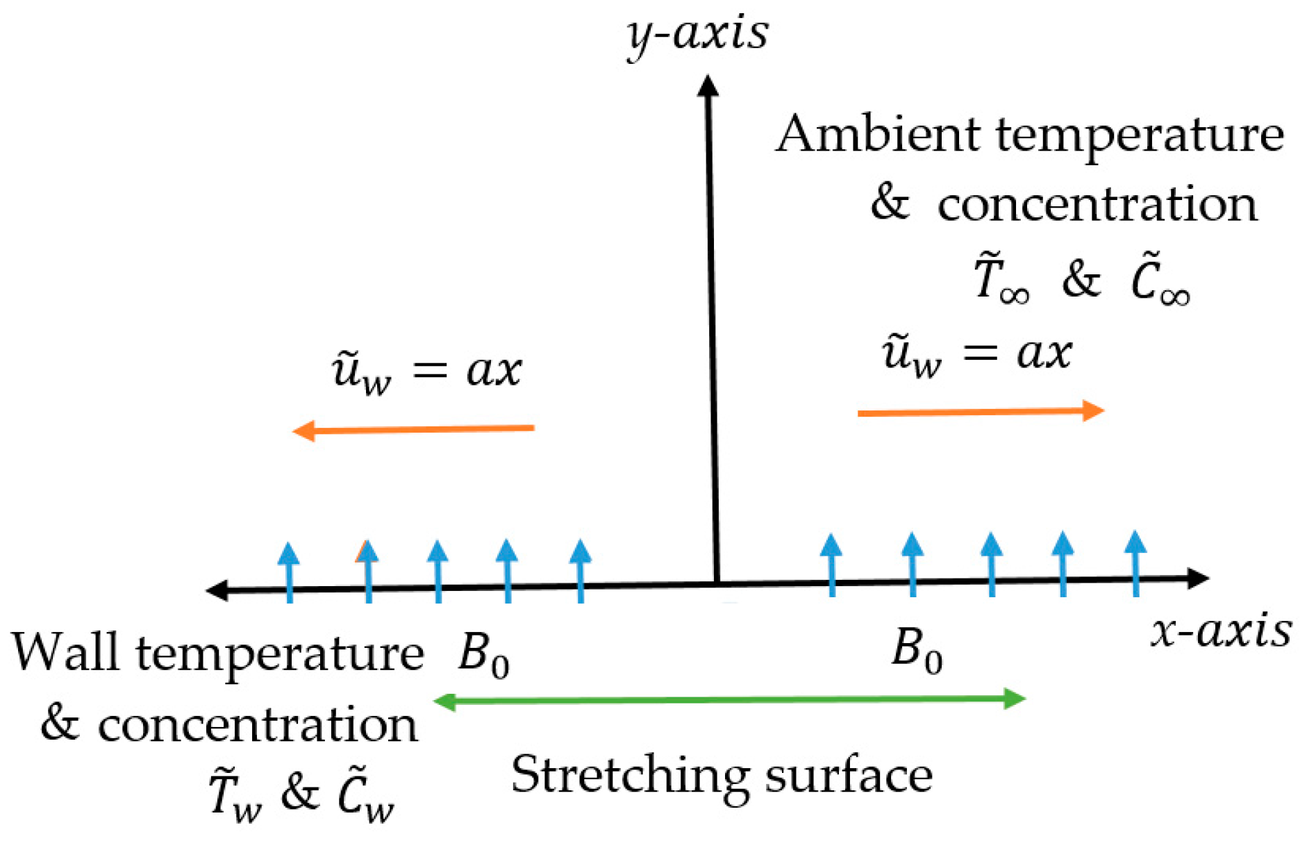
2. Mathematical Formulation

Consider the MHD boundary layer flow of an Eyring–Powell nanofluid over a permeable stretching surface near a stagnation point at $y=0$. The MHD flow occurs in the domain at $y>0.$ The fluid is electrically conducting due to an externally applied magnetic field, although the induced magnetic charge is very small, and is thereby taken to be zero. A cartesian coordinate is chosen in a way such that the x-axis is considered along the direction of the sheet whereas the y-axis is considered normal to it (see Figure 1). Suppose that ${\tilde{T}}_w$ and ${\tilde{C}}_w$ are the temperature and nanoparticle fraction at the sheet, respectively, while the temperature and nano-particle fraction at infinity are ${\tilde{T}}_{\infty }$ and ${\tilde{C}}_{\infty }$, respectively. The velocity of the sheet is considered along the x-direction.

The governing equations of the MHD Eyring–Powell nanofluid model can be written as [35]

$$\frac{\partial \tilde{u}}{\partial x}+\frac{\partial \tilde{v}}{\partial y}=0,$$

(1)

$$\tilde{u}\frac{\partial \tilde{u}}{\partial x}+\tilde{v}\frac{\partial \tilde{v}}{\partial y}=(v+\frac{1}{\rho BC})\frac{{\partial }^2\tilde{u}}{\partial y^2}-\frac{1}{2\rho B{C}^3}{\left(\frac{\partial \tilde{u}}{\partial y}\right)}^2\frac{{\partial }^2\tilde{u}}{\partial y^2}+{\tilde{u}}_e\frac{d{\tilde{u}}_e}{dx}+\frac{\sigma B_0^2}{\rho }({\tilde{u}}_e-\tilde{u}),$$

(2)

$$\tilde{u}\frac{\partial \tilde{T}}{\partial x}+\tilde{v}\frac{\partial \tilde{T}}{\partial y}=\overline{\alpha }\frac{{\partial }^2\tilde{T}}{\partial y^2} +\tau \left(D_B\frac{\partial \tilde{C}}{\partial y}\frac{\partial \tilde{T}}{\partial y}+\frac{D_T}{T_{\infty }}{\left(\frac{\partial \tilde{T}}{\partial y}\right)}^2\right)-\frac{1}{\rho c_p}\frac{\partial q_r}{\partial y},$$

(3)

$$\tilde{u}\frac{\partial \tilde{C}}{\partial x}+\tilde{v}\frac{\partial \tilde{C}}{\partial y}=D_B\frac{{\partial }^2\tilde{C}}{\partial y^2}+\frac{D_T}{T_{\infty }}\frac{{\partial }^2\tilde{T}}{\partial y^2}.$$

(4)

The nonlinear radiative heat flux can be written as

$$q_r=-\frac{4\overline{\sigma }}{3\overline{k}} \frac{\partial {\tilde{T}}^4}{\partial y}=-\frac{16\overline{\sigma }{\tilde{T}}^3}{3\overline{k}}\frac{\partial \tilde{T}}{\partial y},$$

(5)

and their respective boundary conditions are

$$\tilde{u}=u_w=ax, \tilde{v}={\tilde{v}}_w, \tilde{T}={\tilde{T}}_w, \tilde{C}={\tilde{C}}_w\text{ at }y=0,$$

(6)

$$\tilde{u}={\tilde{u}}_e=bx, \tilde{v}=0, \tilde{T}\to {\tilde{T}}_{\infty }, \tilde{C}\to {\tilde{C}}_{\infty }\text{ as }y\to \infty ,$$

(7)

where $b=a$ is considered for the present study. The steam function satisfying Equation (1) is defined as $\left(\tilde{u},\tilde{v}\right)=\left(\frac{\partial \phi }{\partial y},-\frac{\partial \phi }{\partial x}\right)$. Defining the following similarity transformation variables

$$\zeta =\sqrt{\frac{{\tilde{u}}_w}{\nu x} }y, \tilde{u}={\tilde{u}}_w{f}^{\prime }\left(\zeta \right),\phi =\sqrt{a\nu }xf\left(\zeta \right),\tilde{v}=-\sqrt{\frac{\nu {\tilde{u}}_w}{x}}f\left(\zeta \right), \theta =\frac{\tilde{T}-{\tilde{T}}_{\infty } }{{\tilde{T}}_w-{\tilde{T}}_{\infty }},$$

$$\varphi =\frac{\tilde{C}-{\tilde{C}}_{\infty } }{{\tilde{C}}_w-{\tilde{C}}_{\infty }},$$

(8)

and using Equation (8) in relation to Equations (1)–(7), we get

$$\left(1+\gamma \right)f^{‴}+1-\gamma \beta {(f^{″})}^2 f^{‴}-f^{\prime 2}+f{f}^{″}+M\left(1-f^{\prime }\right)=0,$$

(9)

$$\left(\frac{1}{Pr}+N_r\right){\theta }^{″}+f{\theta }^{\prime }+N_b{\theta }^{\prime }{\varphi }^{\prime }+N_t{\left({\theta }^{\prime }\right)}^2=0,$$

(10)

$${\varphi }^{″}+L_{e}f{\varphi }^{\prime }+\frac{N_t}{N_b}{\theta }^{″}=0.$$

(11)

Their corresponding boundary conditions are

$$f\left(0\right)=S, f^{\prime }\left(0\right)=\alpha , f^{\prime }\left(\infty \right)=1,$$

(12)

$$\theta \left(0\right)=1, \theta \left(\infty \right)=0,$$

(13)

$$\varphi \left(0\right)=1,\varphi \left(\infty \right)=0,$$

(14)

where $Pr=\frac{v}{\overline{a}}M=\frac{B_0^2\sigma }{a\rho }{L}_e=\frac{v}{D_B},N_b=\frac{\tau D_B\left({\varphi }_w-{\varphi }_{\infty }\right)}{v},N_t=\frac{\tau D_T\left({\tilde{T}}_w-{\tilde{T}}_{\infty }\right)}{{\tilde{T}}_{\infty }v},N_r=\frac{16\overline{\sigma }{\tilde{T}}^3}{3\rho c_p\overline{k}},\gamma =\frac{1}{\mu BC},\beta =\frac{{\left(ax\right)}^3}{2xv{C}^2}$.

3. Physical Quantities of Interest

The physical quantities of interest for the governing flow problem are the local Nusselt number and local Sherwood number which can be written as

$$N{u}_x=\frac{x{q}_w}{\kappa ({\tilde{T}}_w-{\tilde{T}}_{\infty })}, S{h}_x=\frac{x{q}_m}{D_B(C_w-C_{\infty })},$$

(15)

where $q_w$ and $q_m$ are described as

$$q_w= -\kappa \left(\overline{\alpha }+\frac{16\overline{\sigma }{\tilde{T}}^3}{3\overline{k}}\frac{\partial \tilde{T}}{\partial y}\right){\left(\frac{\partial \tilde{T}}{\partial y}\right)}_{y=0}, q_m=D_B{\left(-\frac{\partial C}{\partial y}\right)}_{y=0}.$$

(16)

With the help of dimensionless transformation in Equation (8), we have

$$N{u}_r=\frac{N{u}_x}{{\text{Re}}_x^{\frac{1}{2}}}= -\left(1+N_r\right){\theta }^{\prime }\left(0\right), S{h}_r=\frac{S{h}_x}{{\text{Re}}_x^{\frac{1}{2}}}=-{\varphi }^{\prime }\left(0\right),$$

(17)

where $S{h}_r$ and $N{u}_r$ are the dimensionless Sherwood number and local Nusselt number, respectively, and ${\text{Re}}_x={\tilde{u}}_{w}x/\nu$ is the local Reynolds number.

4. Numerical Method

We apply the Successive linearization method to Equation (9) with their boundary conditions in Equation (12), by setting [19,25]

$$f\left(\zeta \right)=f_I\left(\zeta \right)+{\displaystyle \sum }_{N=0}^{I-1}{f}_N\left(\zeta \right), \left(I=1,2,3,\dots \right),$$

(18)

where $f_I$ are unknown functions which are obtained by iteratively solving the linearized version of the governing equation and assuming that $f_I \left(0\le N\le I-1\right)$ are known from previous iterations. Our algorithm starts with an initial approximation $f_0$ which satisfies the given boundary conditions in Equation (13) according to SLM. The suitable initial guess for the governing flow problem is

$$f_0=-1+\frac{1-\alpha }{e^{\zeta }}+\zeta +\alpha +S.$$

(19)

We write the equation in general form as

$$L\left(f,f^{\prime },f^{″},f^{‴}\right)+N\left(f,f^{\prime },f^{″},f^{‴}\right)=0,$$

(20)

where

$$L\left(f,f^{\prime },f^{″},f^{‴}\right)=f^{‴},$$

(21)

and

$$N\left(f,f^{\prime },f^{″},f^{‴}\right)=1-\gamma \beta {(f^{″})}^2{f}^{‴}-f^{\prime 2}+f{f}^{″}+M\left(1-f^{\prime }\right),$$

(22)

where $L$ and $N$ are the linear and non-linear part of Equation (9). By substituting Equation (18) into Equation (9) and taking the linear terms only, we get

$$f_I^{‴}+A_{0,I-1}{f}_I^{″}+A_{1,I-1}{f}_I^{\prime }+A_{2,I-1}{f}_I=r_{I-1},$$

(23)

and the corresponding boundary conditions becomes

$$f_I\left(0\right)=0, f_I^{\prime }\left(0\right)=0,f_I\prime \left(\infty \right)=0.$$

(24)

We solve Equation (23) numerically by the Chebyshev spectral collocation method. For numerical implementation, the physical region $\left[0,\infty \right)$ is truncated to $\left[0,\mathrm{\Gamma }\right];$ we can take $\mathrm{\Gamma }$ to be sufficient large. With the help of subsequent transformations this region is further transformed into $\left[-1,1\right]$, and we have

$$\mathrm{\Omega }=-1+\frac{2\zeta }{\mathrm{\Gamma }}.$$

(25)

We define the following discretization between the interval $\left[-1,1\right]$. Now, we can apply Gause–Lobatto collocation points to define the nodes between $\left[-1,1\right]$ by

$${\mathrm{\Omega }}_J=\cos \frac{\pi J}{N}, \left(J=0,1,2,3\dots N\right),$$

(26)

with $\left(N+1\right)$ number of collocation points. The Chebyshev spectral collocation method is based on the concept of differentiation matrix $D$. This differentiation matrix maps a vector of the function values $G={\left[f\left({\mathrm{\Omega }}_0\right),\dots ,f\left({\mathrm{\Omega }}_N\right)\right]}^{\mathit{T}}$ the collocation points to a vector $G^{\prime }$ is defined as

$$G^{\prime }={\displaystyle \sum }_{K-0}^N{D}_{KJ}f\left({\mathrm{\Omega }}_K\right)=DG,$$

(27)

the derivative of$p$order for the function $f\left(\mathrm{\Omega }\right)$ can be written as

$$f^p\left(\mathrm{\Omega }\right)=D^{p}G.$$

(28)

The entries of matrix $D$ can be computed by the method proposed by Bhatti et al. [25]. Now, applying the spectral method, with derivative matrices on linearized Equations (23) and (24), we get the following linearized matrix system

$$A_{I-1}{G}_I=R_{I-1},$$

(29)

and the boundary conditions takes the following form

$$f_I\left({\mathrm{\Omega }}_N\right)=0, {\displaystyle \sum }_{K=0}^N{D}_{NK}{f}_I\left({\mathrm{\Omega }}_K\right)=0,{\displaystyle \sum }_{K=0}^N{D}_{\mathbf{0}K}{f}_I\left({\mathrm{\Omega }}_K\right)=0,{\displaystyle \sum }_{K=0}^N{D}_{\mathbf{0}K}^{\mathbf{2}}{f}_I\left({\mathrm{\Omega }}_K\right)=0,$$

(30)

where

$$A_{I-1}=D^{\mathbf{3}}+A_{0,I-1}{D}^{\mathbf{2}}+A_{1,I-1}D+A_{2,I-1}.$$

(31)

In the above equation $A_{s,I-1}\left(s=0,1,\dots 3\right)$ are $\left(N+1\right)\times \left(N+1\right)$ diagonal matrices with $A_{s,I-1}\left({\mathrm{\Omega }}_J\right)$ on the main diagonal and

$$G_I=f_I\left({\mathrm{\Omega }}_J\right), R_I=r_I\left({\mathrm{\Omega }}_J\right). \left(J=0,1,2,3,\dots N\right)$$

(32)

After employing Equation (31), the solutions for $f_I$ are obtained by iteratively solving Equation (30). We obtain the solution for $f\left(\zeta \right)$ from solving Equation (31) and Equations (10) and (11) are now linear; therefore we will apply Chebyshev pseudo-spectral method directly, and by doing so we get

$$BH=S,$$

(33)

with their corresponding boundary conditions boundary conditions

$$\theta \left({\mathrm{\Omega }}_N\right)=1,\theta \left({\mathrm{\Omega }}_0\right)=0,$$

(34)

$$\varphi \left({\mathrm{\Omega }}_N\right)=1,\varphi \left({\mathrm{\Omega }}_0\right)=0,$$

(35)

where $H=\left(\theta \left({\mathrm{\Omega }}_J\right),\varphi \left({\mathrm{\Omega }}_J\right)\right)$, $B$is the set of linear coupled equations of temperature and nanoparticle concentration, $S$ is a vector of zeros, and all vectors in Equation (33) are converted to a diagonal matrix. We imposed the boundary conditions in Equations (34) and (35) on the first and last rows of $B$ and $S$, respectively.

5. Entropy Generation Analysis

The volumetric entropy generation of the Eyring–Powell nanofluid is given by [36]

$$S_{gen}^{‴}=\frac{\kappa }{{\tilde{T}}_{\infty }^2}\left[{\left(\frac{\partial \tilde{T}}{\partial y}\right)}^2+\frac{16\overline{\sigma }{\tilde{T}}^3}{3\overline{k}}{\left(\frac{\partial \tilde{T}}{\partial y}\right)}^2\right]+\frac{\mu }{{\tilde{T}}_{\infty }^{}}\left(\left(1+\frac{1}{\rho BC}\right){\left(\frac{\partial \tilde{u}}{\partial \tilde{y}}\right)}^2-\frac{1}{6\rho BC}{\left(\frac{\partial \tilde{u}}{\partial y}\right)}^4\right)+\frac{RD}{C_{\infty }}{\left(\frac{\partial C}{\partial y}\right)}^2+\frac{\sigma B_0^2}{{\tilde{T}}_{\infty }}{\tilde{u}}^2+\frac{RD}{{\tilde{T}}_{\infty }}\left(\frac{\partial \tilde{T}}{\partial y}\frac{\partial C}{\partial y}+\frac{\partial C}{\partial x}\frac{\partial \tilde{T}}{\partial x}\right).$$

(36)

In the above equation, the entropy generation consists of three effects: (i) conduction effect (also known as heat transfer irreversibility, (HTI)); (ii) fluid friction irreversibility (FFI); and (iii) diffusion (also known as diffusive irreversibility, (DI)). The entropy generation characteristics can be written as

$$S_0^{‴}=\frac{\kappa {\left(\mathrm{\Delta }T\right)}^2}{L^2{\tilde{T}}_{\infty }^2 }.$$

(37)

With the help of Equation (8), the entropy generation in dimensionless form can be written as

$$\begin{gathered} N_G=\frac{S_{gen}^{‴}}{S_0^{‴}}=\mathrm{Re}\left(1+N_r\right){\theta }^{\prime 2}\left(\zeta \right)+\frac{\mathrm{Re}{B}_r}{\Omega }\left(\left(1+\gamma \right)f^{″2}\left(\zeta \right)-\frac{\gamma \beta }{3}{f}^{″4}\left(\zeta \right)\right) \\ +\frac{\mathrm{Re}{B}_r}{\Omega }M{f}^{\prime 2}\left(\zeta \right)+\mathrm{Re}{\lambda }_1{\left(\frac{\chi }{\Omega }\right)}^2{\varphi }^{\prime 2}\left(\zeta \right)+\mathrm{Re}{\lambda }_1\left(\frac{\chi }{\Omega }\right){\theta }^{\prime }\left(\zeta \right){\varphi }^{\prime }\left(\zeta \right). \end{gathered}$$

(38)

These numbers are given in the following form

$$\text{Re}=\frac{{\tilde{u}}_L{L}^2}{\nu }, B_r=\frac{\mu {\tilde{u}}_w{}^2}{\kappa \mathrm{\Delta }T}, \mathrm{\Omega }=\frac{\mathrm{\Delta }T}{{\tilde{T}}_{\infty }}, \chi =\frac{\mathrm{\Delta }C}{C_{\infty }}, {\lambda }_1=\frac{RD{C}_{\infty }}{\kappa }.$$

(39)

6. Results and Discussion

This section deals with the theoretical and graphical behavior of different physical quantities that are obtained in the present flow problems. The computational software Matlab has been utilized to investigate the novelties of all the physical parameters, such as the Hartmann number, fluid parameter, Prandtl number, radiation parameter, Lewis number, thermophoresis parameter, Brownian motion parameter, Reynolds number, and Brinkmann number. In particular, we discuss their influence on velocity profile, temperature profile, nanoparticle concentration profile, and entropy profile. For this purpose, Figure 1, Figure 2, Figure 3, Figure 4, Figure 5, Figure 6, Figure 7, Figure 8, Figure 9 and Figure 10 are drawn, where Figure 1 shows the geometry of the problem.

Table 1. Numerical values of reduced Nusselt number and local Sherwood number for various values of $Pr, N_r, N_b, L_e,\text{ and }{N}_t$.

$\mathit{P}\mathit{r}$	${\mathit{N}}_{\mathit{r}}$	${\mathit{N}}_{\mathit{b}}$	${\mathit{N}}_{\mathit{t}}$	${\mathit{L}}_{\mathit{e}}$	$\mathit{N}{\mathit{u}}_{\mathit{r}}$	$\mathit{S}{\mathit{h}}_{\mathit{r}}$
1	1	-	-	-	1.4998	-
2		-	-	-	1.7638	-
10		-	-	-	2.0890	-
-	2	-	-	-	2.1308	-
-	3	-	-	-	2.2947	-
-	4	-	-	-	2.4657	-
-	-	0.1	-	-	2.0890	0.6456
-	-	0.3	-	-	1.9087	0.9680
-	-	0.8	-	-	1.5922	1.1944
-	-	-	0.2	-	1.9936	0.8506
-	-	-	0.4	-	1.8325	0.6456
-	-	-	0.7	-	1.6444	0.4996
-	-	-	-	1.5	-	1.1386
-	-	-	-	2	-	1.4137
-	-	-	-	3	-	1.9450

shows the numerical computation of the Nusselt number and Sherwood number for different values of the Prandtl number, radiation parameter, Brownian motion parameter, thermophoresis parameter, and Lewis number.

Table 2. Comparison of $f^{″}\left(0\right)$ with existing published data for different values of stretching parameter $\alpha >0$.

$\mathit{\alpha }$	Present Results $\mathit{\gamma }=\mathit{M}=\mathbf{0}$	Wang [37]
0	1.23258	1.23258
0.1	1.14656	1.14656
0.2	1.05113	1.05113
1	0.00000	0.00000
2	−1.88730	−1.88730
5	−10.26474	−10.26474

represents a numerical comparison with the existing published results [26] by taking $\gamma =M=0$ as a special case of our study. From this table, we can see that our results are in excellent agreement, which confirms the validity of our present methodology.

Figure 2 and Figure 3 are provided for the velocity profile against Hartman number $\left(M\right)$, fluid parameter $\left(\gamma \right),$ and suction/injection parameter $\left(S\right)$. Figure 2 elucidates that when the Hartmann number $\left(M\right)$ increases then it opposes the flow which causes a reduction in the fluid velocity. In fact, this is due to the existence of the Lorentz force which originated when the magnetic field was applied. However, we can observe that suction/injection parameter $\left(S\right)$ does not provide any resistance to the flow, and hence the velocity of the fluid tends to rise when the suction/injection parameter increases. Figure 3 shows that when the fluid parameter $\left(\gamma \right)$ rises then it tends to oppose the flow, which causes a reduction in the velocity profile. Figure 4 and Figure 5 are provided for the temperature profile against Brownian motion parameter, thermophoresis parameter, Prandtl number, and radiation parameter. It can be observed from Figure 4 that the Brownian motion parameter $\left(N_b\right)$ enhances the temperature profile and boundary layer thickness, however, the temperature profile behaves in a similar way when the thermophoresis parameter $\left(N_t\right)$ increases. An enhancement in the thermophoresis parameter produces a force which leads to the movement of nanoparticles from a hot region to cold region, and hence the temperature profile and thermal boundary layer thickness increases. It can be observed from Figure 5 that the radiation parameter $\left(N_r\right)$ enhances the temperature profile. In fact, this happens due to the increment in radiation parameter causing a reduction in the mean absorption coefficient, which, as a result, leads to an increase in the radiative heat transfer. Here we can also observe that larger values of the Prandtl number reduces the temperature profile and the boundary layer thickness. An increment in the Prandtl number coincides with weaker thermal diffusivity. It is worth mentioning that those fluids which hold weaker thermal diffusivity have lower temperatures. This type of thermal diffusivity reveals a reduction in the boundary layer thickness and temperature profile.

Figure 6 and Figure 7 are provided for the concentration profile against the Brownian motion parameter, thermophoresis parameter, Lewis number, and suction/injection parameter. Figure 6 shows that an increment in the Lewis number $\left(L_e\right)$ tends to reduce the concentration profile and its boundary layer thickness. Moreover, the concentration profile and boundary thickness behave in a similar way when the suction parameter $\left(S\right)$ increases. From Figure 7, we can observe that an increment in the Brownian motion parameter $\left(N_b\right)$ tends to decrease the boundary layer thickness and nanoparticle concentration profile; however, the nanoparticle concentration profile behaves in an opposite way when the thermophoresis parameter $\left(N_t\right)$ increases. Figure 8, Figure 9 and Figure 10 represent the entropy profile for the Reynolds number, Brinkmann number, radiation parameter, and Hartmann number. In Figure 8 we can easily notice that the entropy profile decreases due to the increment in radiation parameter $\left(N_r\right)$; however, when $\zeta \to \infty$ then its behavior starts to change and becomes the opposite after certain values of $\zeta$. It can be observed from Figure 9 and Figure 10 that the entropy profile increases correspondingly with increasing values for the Reynolds number, Brinkmann number, and Hartmann number.

7. Conclusions

Entropy generation of an Eyring–Powell nanofluid through a permeable stretching surface has been investigated numerically. The impact of MHD and nonlinear thermal radiation are also taken into consideration. The solution of the governing flow problem has been obtained with the help of the Successive linearization method and Chebyshev spectral collocation method. The major outcomes are summarized below:

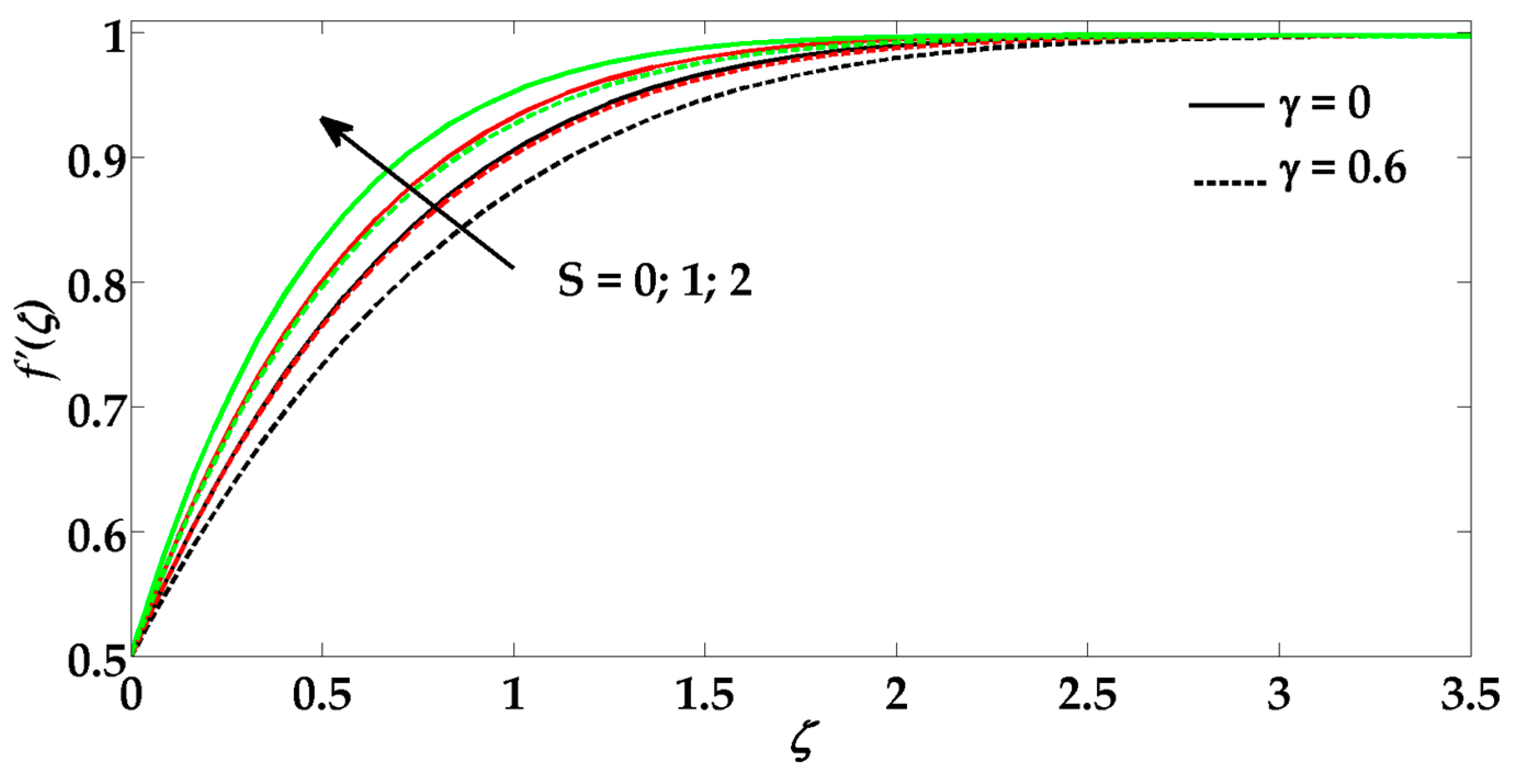
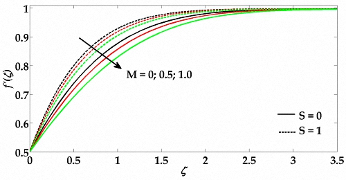
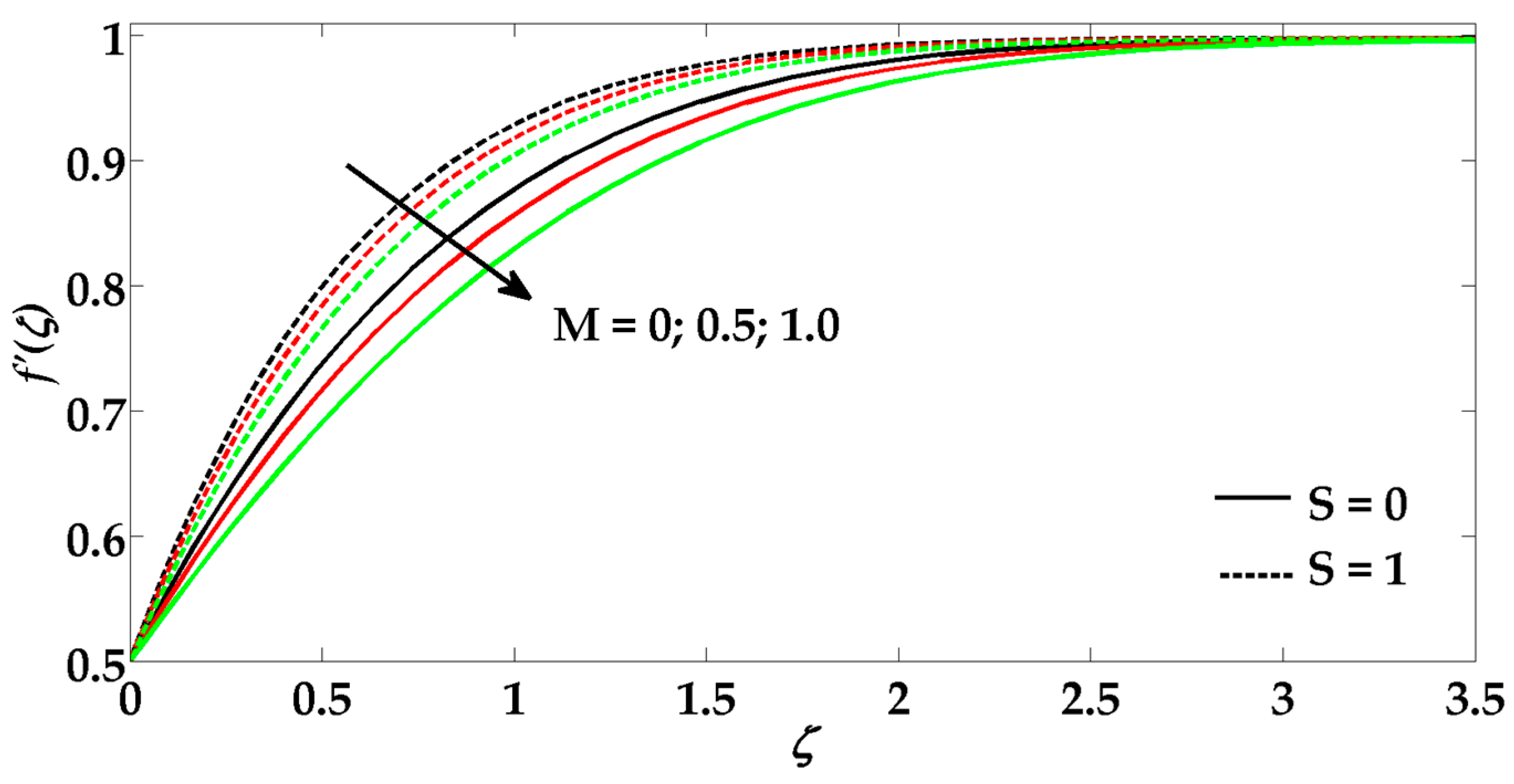
• The velocity of the fluid decreases due to an increment in the fluid parameter and Hartmann number.
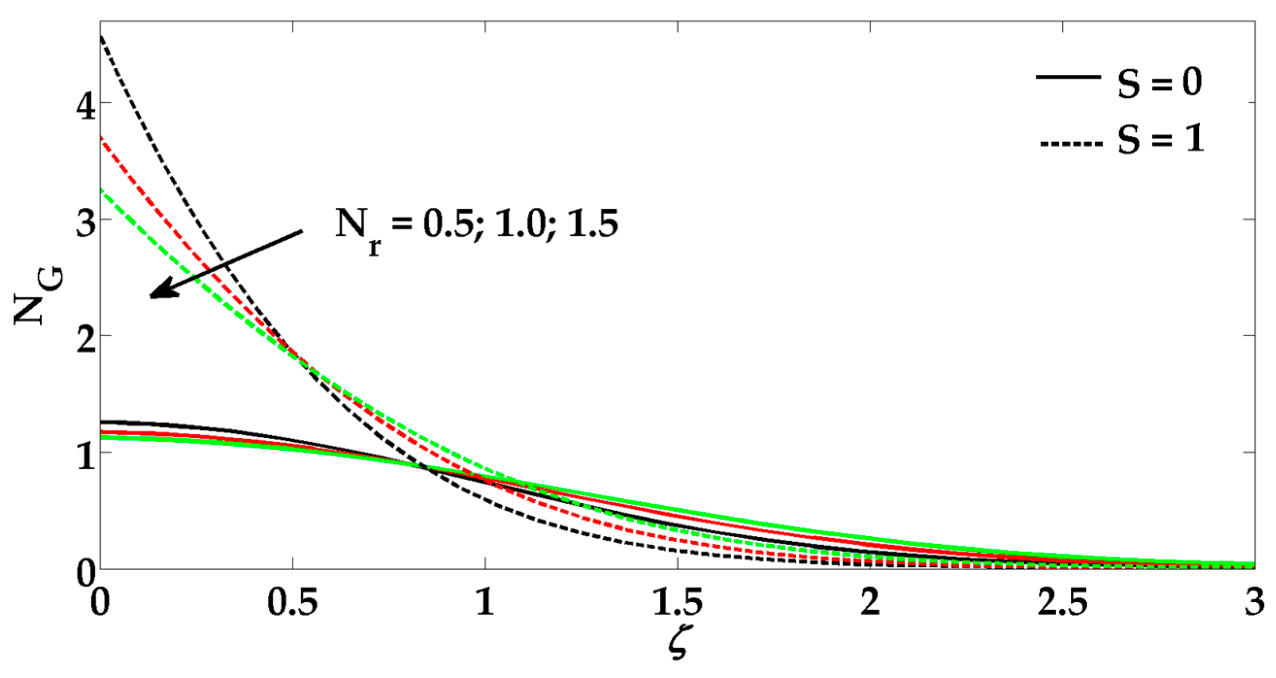
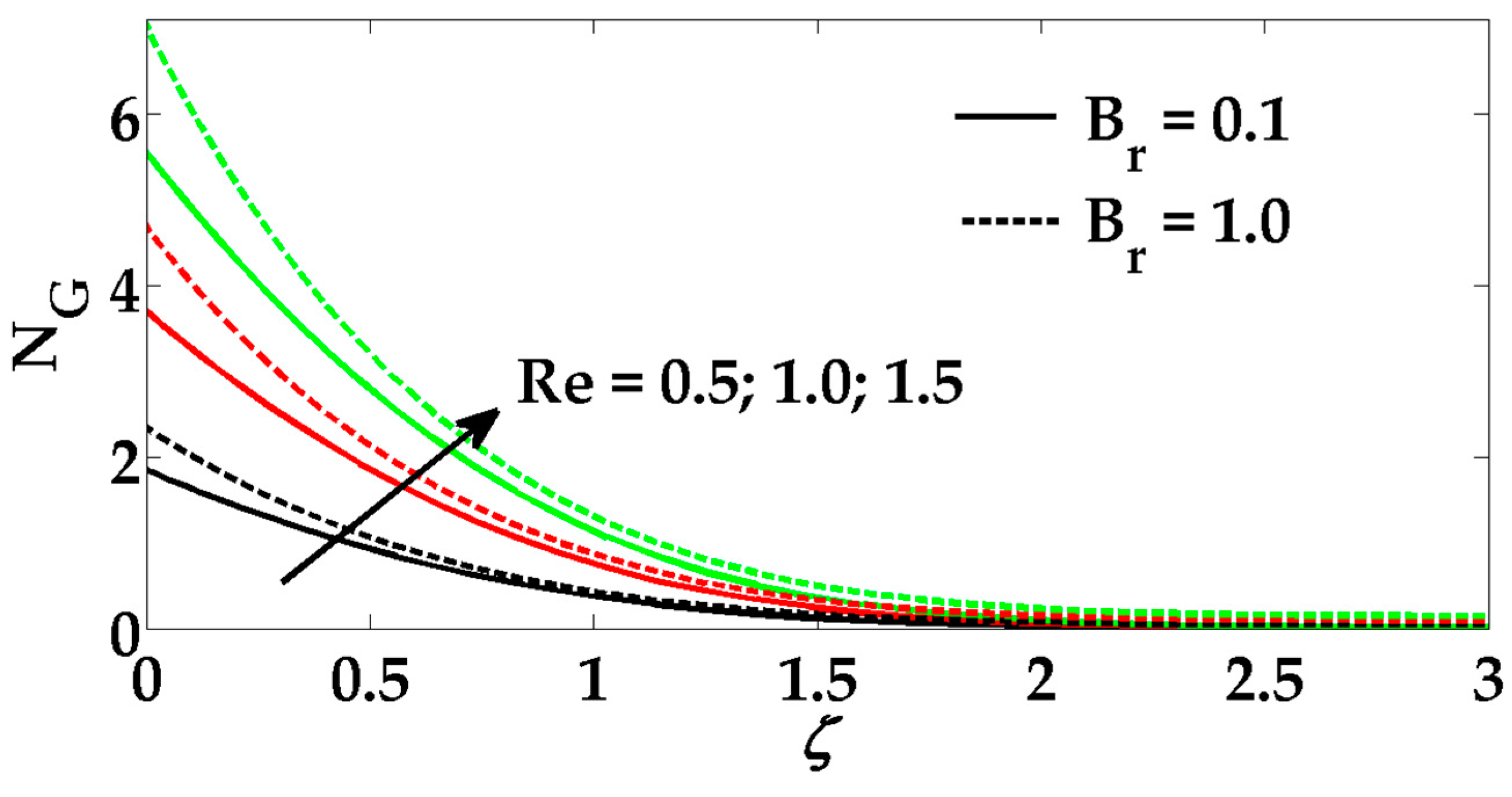
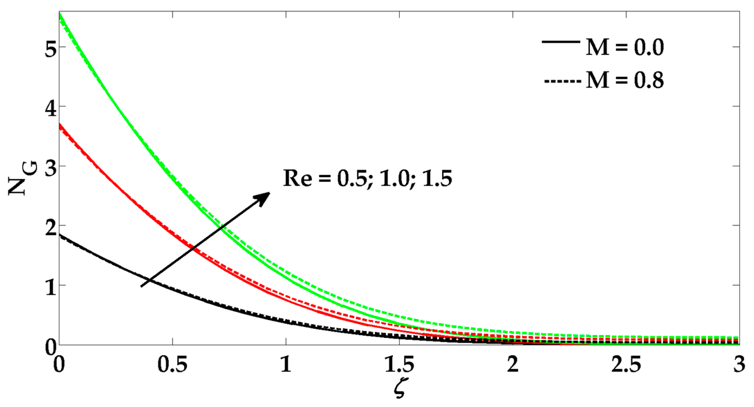
• The entropy profile enhances all the physical parameters.
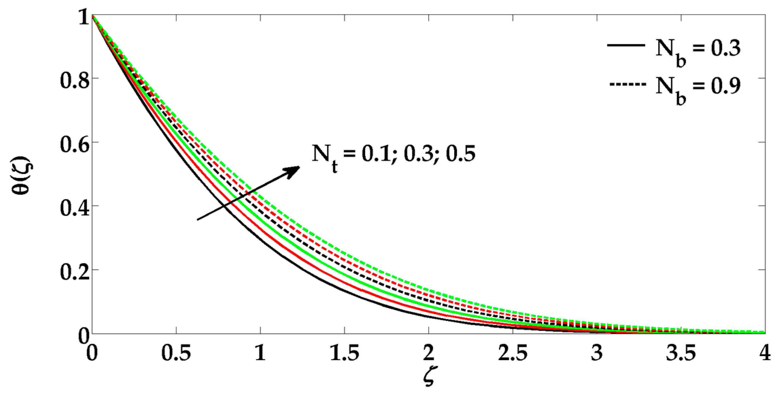
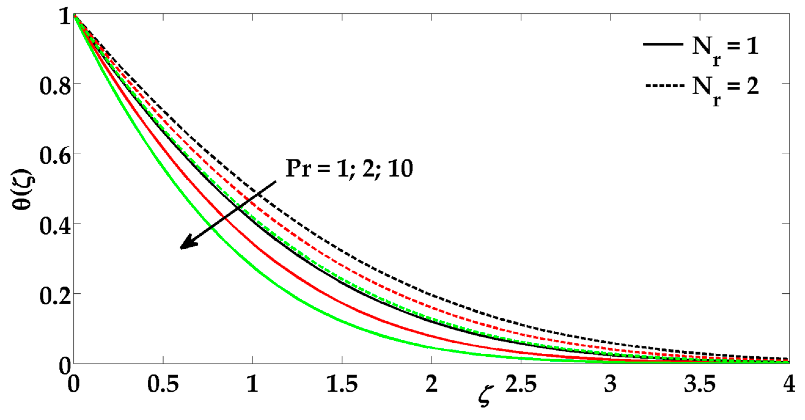
• The temperature profile increases due to an increment in the radiation parameter.
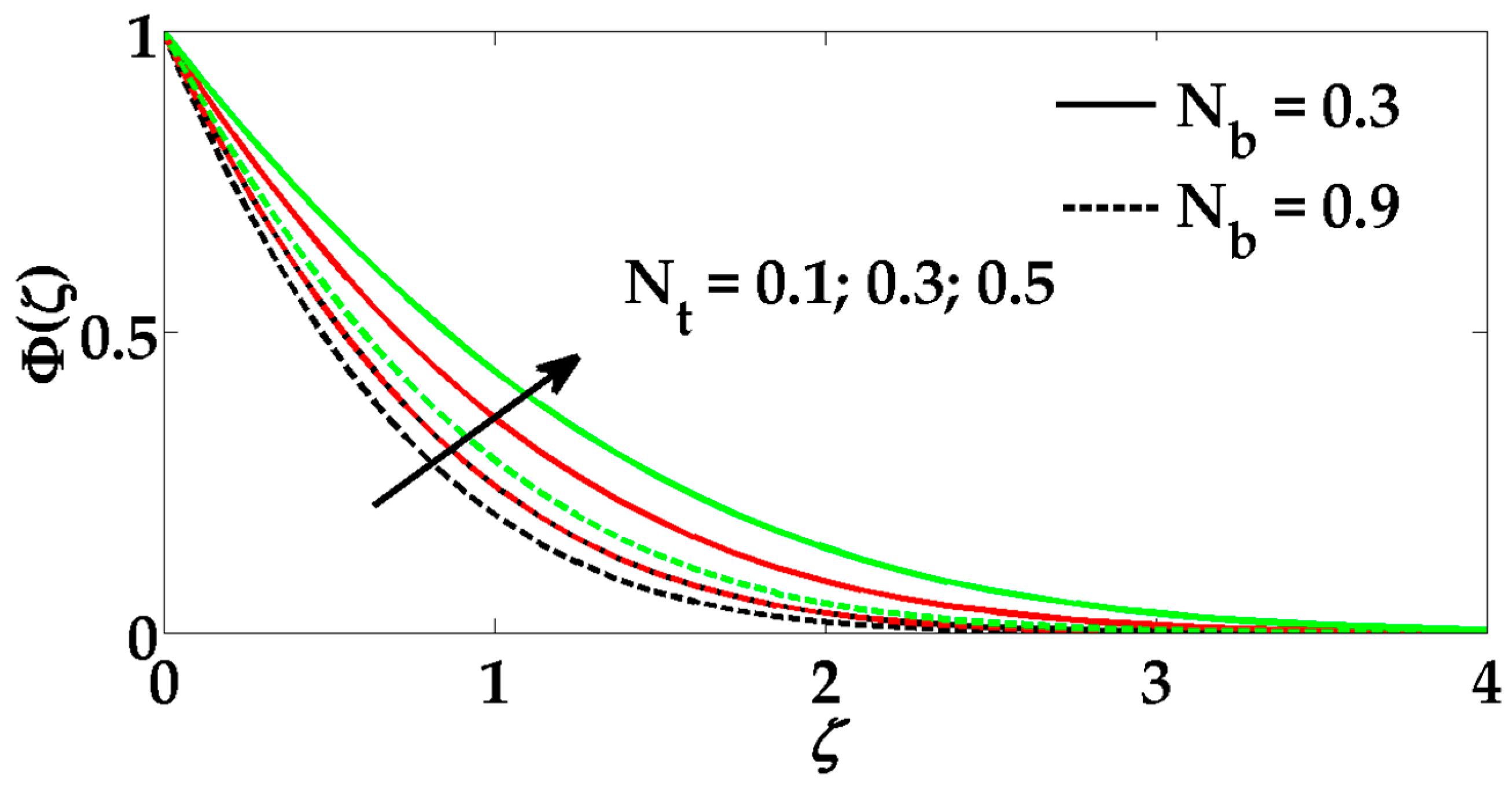
• The nanoparticle concentration increases for large values of the thermophoresis parameter.
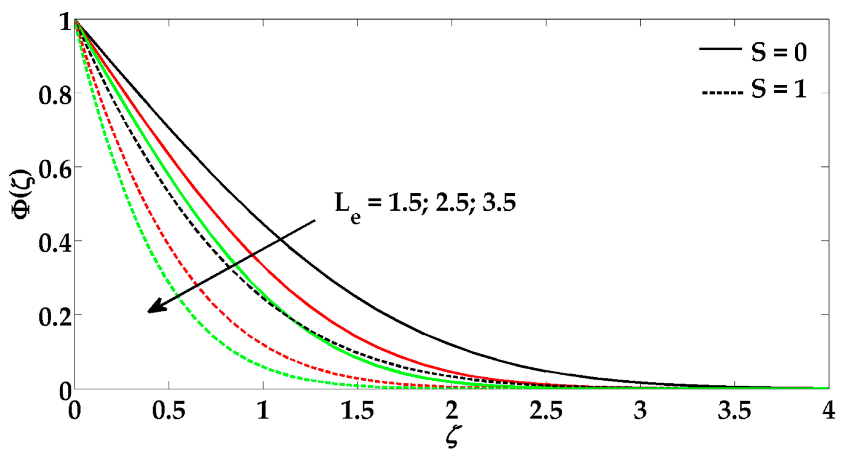
• The nanoparticle concentration decreases due to a greater influence of the Lewis number.

References

1. Choi, S.U.S.; Eastman, J.A. Enhancing Thermal Conductivity of Fluids with Nanoparticles; Technical Report; Argonne National Laboratory: Argonne, IL, USA, October 1995; pp. 99–106. [Google Scholar]
2. Xuan, Y.; Li, Q. Investigation on convective heat transfer and flow features of nanofluids. J. Heat Transf. 2003, 125, 151–155. [Google Scholar] [CrossRef]
3. Buongiorno, J. Convective transport in nanofluids. J. Heat Transf. 2006, 128, 240–250. [Google Scholar] [CrossRef]
4. Eastman, J.A.; Choi, S.U.S.; Li, S.; Yu, W.; Thompson, L.J. Anomalously increased effective thermal conductivities of ethylene glycol-based nanofluids containing copper nanoparticles. Appl. Phys. Lett. 2001, 78, 718–720. [Google Scholar] [CrossRef]
5. Eastman, J.A.; Choi, U.S.; Li, S.; Thompson, L.J.; Lee, S. Enhanced thermal conductivity through the development of nanofluids. In MRS Proceedings; Cambridge University Press: Cambridge, UK, 1996; Volume 457. [Google Scholar]
6. Makinde, O.D.; Khan, W.A.; Khan, Z.H. Buoyancy effects on MHD stagnation point flow and heat transfer of a nanofluid past a convectively heated stretching/shrinking sheet. Int. J. Heat Mass Transf. 2013, 62, 526–533. [Google Scholar] [CrossRef]
7. Bachok, N.; Ishak, A.; Pop, I. Unsteady boundary-layer flow and heat transfer of a nanofluid over a permeable stretching/shrinking sheet. Int. J. Heat Mass Transf. 2012, 55, 2102–2109. [Google Scholar] [CrossRef]
8. Nazar, R.; Jaradat, M.; Arifin, N.; Pop, I. Stagnation-point flow past a shrinking sheet in a nanofluid. Open Phys. 2011, 9, 1195–1202. [Google Scholar] [CrossRef]
9. Malvandi, A.; Hedayeti, F.; Ganji, D.D.; Rostamiyan, Y. Unsteady boundary-layer flow of nanofluid past a permeable stretching/shrinking sheet with convective heat transfer. Proc. Inst. Mech. Eng. Part C J. Mech. Eng. Sci. 2013. [Google Scholar] [CrossRef]
10. Akbar, N.S.; Khan, Z.H.; Nadeem, S. The combined effects of slip and convective boundary conditions on stagnation-point flow of CNT suspended nanofluid over a stretching sheet. J. Mol. Liq. 2014, 196, 21–25. [Google Scholar] [CrossRef]
11. Nadeem, S.; Mehmood, R.; Akbar, N.S. Optimized analytical solution for oblique flow of a Casson-nano fluid with convective boundary conditions. Int. J. Therm. Sci. 2014, 78, 90–100. [Google Scholar] [CrossRef]
12. Zeeshan, A.; Majeed, A.; Ellahi, R. Effect of magnetic dipole on viscous ferro-fluid past a stretching surface with thermal radiation. J. Mol. Liq. 2016, 215, 549–554. [Google Scholar] [CrossRef]
13. Bejan, A. Entropy Generation Minimization: The Method of Thermodynamic Optimization of Finite-Size Systems and Finite-Time Processes; CRC Press: Boca Raton, FL, USA, 1996. [Google Scholar]
14. Bejan, A. Entropy generation minimization: The new thermodynamics of finite-size devices and finite-time processes. J. Appl. Phys. 1996, 79, 1191–1218. [Google Scholar] [CrossRef]
15. Oztop, H.F.; Al-Salem, K. A review on entropy generation in natural and mixed convection heat transfer for energy systems. Renew. Sustain. Energy Rev. 2012, 16, 911–920. [Google Scholar] [CrossRef]
16. Ozawa, H.; Ohmura, A.; Lorenz, R.D.; Pujol, T. The second law of thermodynamics and the global climate system: A review of the maximum entropy production principle. Rev. Geophys. 2003, 41. [Google Scholar] [CrossRef]
17. Abolbashari, M.H.; Freidoonimehr, N.; Nazari, F.; Rashidi, M.M. Analytical modeling of entropy generation for Casson nano-fluid flow induced by a stretching surface. Adv. Powder Technol. 2015, 26, 542–552. [Google Scholar] [CrossRef]
18. Rashidi, M.M.; Abelman, S.; Mehr, N.F. Entropy generation in steady MHD flow due to a rotating porous disk in a nanofluid. Int. J. Heat Mass Transf. 2013, 62, 515–525. [Google Scholar] [CrossRef]
19. Qing, J.; Bhatti, M.M.; Abbas, M.A.; Rashidi, M.M.; Ali, M.E.-S. Entropy Generation on MHD Casson Nanofluid Flow over a Porous Stretching/Shrinking Surface. Entropy 2016, 18. [Google Scholar] [CrossRef]
20. Rashidi, M.M.; Bhatti, M.M.; Abbas, M.A.; Ali, M.E.-S. Entropy Generation on MHD Blood Flow of Nanofluid Due to Peristaltic Waves. Entropy 2016, 18. [Google Scholar] [CrossRef]
21. Abbas, M.A.; Bai, Y.; Rashidi, M.M.; Bhatti, M.M. Analysis of Entropy Generation in the Flow of Peristaltic Nanofluids in Channels with Compliant Walls. Entropy 2016, 18. [Google Scholar] [CrossRef]
22. Sheikholeslami, M.; Ganji, D.D. Entropy generation of nanofluid in presence of magnetic field using Lattice Boltzmann Method. Phys. A Stat. Mech. Appl. 2015, 417, 273–286. [Google Scholar] [CrossRef]
23. Rashidi, M.M.; Ali, M.; Freidoonimehr, N.; Nazari, F. Parametric analysis and optimization of entropy generation in unsteady MHD flow over a stretching rotating disk using artificial neural network and particle swarm optimization algorithm. Energy 2013, 55, 497–510. [Google Scholar] [CrossRef]
24. Abolbashari, M.H.; Freidoonimehr, N.; Nazari, F.; Rashidi, M.M. Entropy analysis for an unsteady MHD flow past a stretching permeable surface in nano-fluid. Powder Technol. 2014, 267, 256–267. [Google Scholar] [CrossRef]
25. Bhatti, M.M.; Shahid, A.; Rashidi, M.M. Numerical simulation of Fluid flow over a shrinking porous sheet by Successive linearization method. Alex. Eng. 2016, 55, 51–56. [Google Scholar] [CrossRef]
26. Abbas, Z.; Sheikh, M.; Motsa, S.S. Numerical solution of binary chemical reaction on stagnation point flow of Casson fluid over a stretching/shrinking sheet with thermal radiation. Energy 2016, 95, 12–20. [Google Scholar] [CrossRef]
27. Hady, F.M.; Ibrahim, F.S.; Abdel-Gaied, S.M.; Eid, M.R. Radiation effect on viscous flow of a nanofluid and heat transfer over a nonlinearly stretching sheet. Nanoscale Res. Lett. 2012, 7, 1–13. [Google Scholar] [CrossRef] [PubMed]
28. Nadeem, S.; Haq, R.U. Effect of thermal radiation for magnetohydrodynamics boundary layer flow of a nanofluid past a stretching sheet with convective boundary conditions. J. Comput. Theor. Nanosci. 2014, 11, 32–40. [Google Scholar] [CrossRef]
29. Rashidi, M.M.; Ganesh, N.V.; Hakeem, A.K.A.; Ganga, B. Buoyancy effect on MHD flow of nanofluid over a stretching sheet in the presence of thermal radiation. J. Mol. Liq. 2014, 198, 234–238. [Google Scholar] [CrossRef]
30. Rashidi, M.M.; Ali, M.; Freidoonimehr, N.; Rostami, B.; Hossain, M.A. Mixed convective heat transfer for MHD viscoelastic fluid flow over a porous wedge with thermal radiation. Adv. Mech. Eng. 2014, 6, 735939. [Google Scholar] [CrossRef]
31. Turkyilmazoglu, M. An analytical treatment for the exact solutions of MHD flow and heat over two–three dimensional deforming bodies. Int. J. Heat Mass Transf. 2015, 90, 781–789. [Google Scholar] [CrossRef]
32. Salahuddin, T.; Malik, M.Y.; Hussain, A.; Bilal, S.; Awais, M. MHD flow of Cattanneo–Christov heat flux model for Williamson fluid over a stretching sheet with variable thickness: Using numerical approach. J. Magn. Magn. Mater. 2016, 401, 991–997. [Google Scholar] [CrossRef]
33. Yasin, M.H.M.; Ishak, A.; Pop, I. MHD heat and mass transfer flow over a permeable stretching/shrinking sheet with radiation effect. J. Magn. Magn. Mater. 2016, 407, 235–240. [Google Scholar] [CrossRef]
34. Ganga, B.; Saranya, S.; Vishnu, G.N.; Abdul, H.A. Effects of space and temperature dependent internal heat generation/absorption on MHD flow of a nanofluid over a stretching sheet. J. Hydrodyn. Ser. B 2015, 27, 945–954. [Google Scholar] [CrossRef]
35. Akbar, N.S.; Ebaid, A.; Khan, Z.H. Numerical analysis of magnetic field effects on Eyring–Powell fluid flow towards a stretching sheet. J. Magn. Magn. Mater. 2015, 382, 355–358. [Google Scholar] [CrossRef]
36. Bhatti, M.M.; Abbas, T.; Rashidi, M.M.; Ali, M.E.-S. Numerical Simulation of Entropy Generation with Thermal Radiation on MHD Carreau Nanofluid towards a Shrinking Sheet. Entropy 2016, 18. [Google Scholar] [CrossRef]
37. Wang, C.Y. Stagnation flow towards a shrinking sheet. Int. J. Non Linear Mech. 2008, 43, 377–382. [Google Scholar] [CrossRef]
Figure 1. Geometry of the problem.
Entropy 18 00224 g001
Figure 2. Velocity profile for different values of M and S when P r = 5 ,   N r = 1 ,   γ = 0.1 ,   β = 0.5 ,   N b = 0.2 ,   N t = 0.2 and L e = 1 . Solid black line: M = 0 ,  S = 0 ; Dashed black line: M = 0 ,  S = 1 ; Solid red line: M = 0.5 ,  S = 0 ; Dashed red line: M = 0.5 ,  S = 1 ; Solid green line: M = 1.0 ,  S = 0 ; Dashed green line: M = 1.5 ,  S = 1 .
Entropy 18 00224 g002
Figure 3. Velocity profile for different values of S and γ when P r = 5 ,   N r = 1 ,   β = 0.6 ,   N b = 0.2 ,   N t = 0.2 ,   L e = 1 and M = 0.1. Solid black line: γ = 0 ,  S = 0 ; Dashed black line: γ = 0.6 ,  S = 0 ; Solid red line: γ = 0 ,  S = 1 ; Dashed red line: γ = 0.6 ,  S = 1 ; Solid green line: γ = 0 ,  S = 2 ; Dashed green line: γ = 0.6 ,  S = 2 .
Entropy 18 00224 g003
Figure 4. Temperature profile for different values of N t and N b when P r = 5 ,   N r = 1 ,   γ = 0.2 ,   β = 0.6 ,   L e = 1 and M = 0.1. Solid black line: N t = 0.1 ,   N b = 0.3 ; Dashed black line: N t = 0.1 ,   N b = 0.9 ; Solid red line: N t = 0.3 ,   N b = 0.3 ; Dashed red line: N t = 0.3 ,   N b = 0.9 ; Solid green line: N t = 0.5 ,   N b = 0.3 ; Dashed green line: N t = 0.5 ,   N b = 0.9.
Entropy 18 00224 g004
Figure 5. Temperature profile for different values of N r and P r when α = 0.9 ,   γ = 0.2 ,   β = 0.6 ,   N b = 0.2 ,   N t = 0.2 ,   L e = 1 and M = 0.1 . Solid black line: P r = 1 ,   N r = 1 ; Dashed black line: P r = 1 ,   N r = 2 ; Solid red line: P r = 2 ,   N r = 1 ; Dashed red line: P r = 2 ,   N r = 2 ; Solid green line: P r = 10 ,   N r = 1 ; Dashed green line: P r = 10 ,   N r = 2 .
Entropy 18 00224 g005
Figure 6. Concentration profile for different values of S and L e when P r = 5 ,   N r = 1 ,   γ = 0.2 ,   β = 0.6 ,   N b = 0.2 ,   N t = 0.2 and M = 0.1 . Solid black line: L e = 1.5 ,   S = 0 ; Dashed black line: L e = 1.5 ,   S = 1 ; Solid red line: L e = 2.5 ,   S = 0 ; Dashed red line: L e = 2.5 ,   S = 1 ; Solid green line: L e = 3.5 ,   S = 0 ; Dashed green line:   L e = 3.5 ,   S = 1 .
Entropy 18 00224 g006
Figure 7. Concentration profile for different values of N t and N b when P r = 5 ,   N r = 1 ,   γ = 0.2 ,   β = 0.6 ,   L e = 1 and M = 0.1. Solid black line: N t = 0.1 ,   N b = 0.3 ; Dashed black line: N t = 0.1 ,   N b = 0.9 ; Solid red line: N t = 0.3 ,   N b = 0.3 ; Dashed red line: N t = 0.3 ,   N b = 0.9 ; Solid green line: N t = 0.5 ,   N b = 0.3 ; Dashed green line: N t = 0.5 ,   N b = 0.9 .
Entropy 18 00224 g007
Figure 8. Entropy profile for different values of S and N r when P r = 5 ,   N r = 1 , γ = 0.2 ,   β = 0.6 ,   N b = 0.2 ,   N t = 0.2 ,   L e = 1 and M = 0.1 . Solid black line: S = 0 ,   N r = 0.5 Dashed black line: S = 1 ,   N r = 0.5 ; Solid red line:   S = 0 ,   N r = 1 ; Dashed red line:   S = 1 ,   N r = 1 ; Solid green line:   S = 0 ,   N r = 1.5 ; Dashed green line:   S = 1 ,   N r = 1.5 .
Entropy 18 00224 g008
Figure 9. Entropy profile for different values of B r   and Re when P r = 5 ,   N r = 1 , γ = 0.2 ,   β = 0.6 ,   N b = 0.2 ,   N t = 0.2 ,   L e = 1 and M = 0.1 . Solid black line:   B r = 0.1 ,  Re = 0.5 ; Dashed black line:   B r = 1 ,  Re = 0.5 ; Solid red line:   B r = 0.1 ,  Re = 1.0 ; Dashed red line:   B r = 1 ,  Re = 1.0 ; Solid green line:   B r = 0.1 ,  Re = 1.5 ; Dashed green line:   B r = 1 ,  Re = 1.5 .
Entropy 18 00224 g009
Figure 10. Entropy profile for different values of Re and M   when P r = 5 ,   N r = 1 ,   γ = 0.2 ,   β = 0.6 ,   N b = 0.2 ,   N t = 0.2 and L e = 1 . Solid black line:   M = 0 ,  Re = 0.5 ; Dashed black line:   M = 0.8 ,  Re = 0.5 ; Solid red line:   M = 0 ,  Re = 1.0 ; Dashed red line:   M = 0.8 ,  Re = 1.0 ; Solid green line:   M = 0 ,  Re = 1.5 ; Dashed green line:   M = 0.8 ,  Re = 1.5 .
Entropy 18 00224 g010