Unified Approach to Thermodynamic Optimization of Generic Objective Functions in the Linear Response Regime

Abstract

While many efforts have been devoted to optimizing the power output for a finite-time thermodynamic process, thermodynamic optimization under realistic situations is not necessarily concerned with power alone; rather, it may be of great relevance to optimize generic objective functions that are combinations of power, entropy production, and/or efficiency. One can optimize the objective function for a given model; generally the obtained results are strongly model dependent. However, if the thermodynamic process in question is operated in the linear response regime, then we show in this work that it is possible to adopt a unified approach to optimizing the objective function, thanks to Onsager’s theory of linear irreversible thermodynamics. A dissipation bound is derived, and based on it, the efficiency associated with the optimization problem, which is universal in the linear response regime and irrespective of model details, can be obtained in a unified way. Our results are in good agreement with previous findings. Moreover, we unveil that the ratio between the stopping time of a finite-time process and the optimized duration time plays a pivotal role in determining the corresponding efficiency in the case of linear response.

1. Introduction

Classical thermodynamics mainly deals with quasistatic processes in which energy dissipation is negligible, and this leads to the Carnot efficiency ${\eta }_{\mathrm{C}}=1-T_{\mathrm{c}}/T_{\mathrm{h}}$, which sets an upper bound for extracting work from two heat reservoirs with temperatures $T_{\mathrm{h}}$ (the hot one) and $T_{\mathrm{c}}$ (the cold one), respectively. For a fixed amount of heat $Q_{\mathrm{h}}$ absorbed from the hot reservoir, the work output W cannot exceed ${\eta }_{\mathrm{C}}{Q}_{\mathrm{h}}$. However, the Carnot efficiency can only be achieved for quasistatic processes, that is to say, the power output of such a process is vanishing. Thus, for any realistic thermodynamic process that is conducted within a finite time, the Carnot efficiency should not be the objective to pursue, and in fact people have proposed objective functions other than efficiency to optimize. For example, the power output is often taken as the objective, and the efficiency at maximum power for various kinds of heat engines and heat transfer laws have been investigated following the work of Curzon and Ahlborn [1], in which a bound of efficiency similar to ${\eta }_{\mathrm{C}}$ was found to be ${\eta }_{\mathrm{CA}}=1-\sqrt{T_{\mathrm{c}}/T_{\mathrm{h}}}$. Recently, investigations on maximum efficiency at a given power and on the controlling protocol for engines to achieve the optimal performance have also attracted much interest [2,3,4,5,6,7]. Besides the power output, there are other suggested objective functions such as (i) the so-called ecological function [8], which is defined as $P-T_{\mathrm{c}}\sigma$, where P is the power output and σ is the entropy production rate of the two heat reservoirs, and the associated efficiency when the ecological function is optimized is well approximated as $({\eta }_{\mathrm{C}}+{\eta }_{\mathrm{CA}})/2$ for endoreversible Carnot engines; (ii) a trade-off function [9], which is defined to be proportional to $\eta P$ with η being the thermodynamic efficiency, and for low-dissipation engines the corresponding efficiency at maximum trade-off is in the range $[2{\eta }_{\mathrm{C}}/3,(3-\sqrt{9-8{\eta }_{\mathrm{C}}})/2]$. In fact, the choice of the objective function is somewhat arbitrary, but typically, the objective function is a combination of P, σ, and η, and the corresponding optimized process lies somewhere in the range between the quasistatic process with no dissipation and the process with maximum power output [10].

For a given model, one can optimize the chosen objective function and obtain the corresponding efficiency. Not surprisingly, it seems that the results are totally model dependent. This is partly due to the fact that the second law of thermodynamics is an inequality rather than an equality, and we lack universally held deterministic equations to describe generic nonequilibrium thermodynamic processes. However, in the regime of linear irreversible thermodynamics, it is possible to treat the power-efficiency issue as a general thermodynamic problem [11], and one can actually obtain theoretical results that are stronger than the Guoy-Stodola theorem [12], thanks to Onsager’s theory [13]. Van den Broeck in his seminal work [14] formulated the work-extraction process in terms of generalized fluxes and forces, and by assuming the linear dependence of fluxes on forces, he managed to find the efficiency at maximum power is indeed bounded from above by ${\eta }_{\mathrm{VdB}}={\eta }_{\mathrm{C}}/2$, which is achieved for a finite-time process without heat leakage between two heat reservoirs. This result is universal in the sense that it depends neither on the types of heat engines nor on the heat transfer laws [15,16]. The only assumption is that during the whole process, the overall system of two heat reservoirs plus the working fluid is operated in the linear response regime, where the Onsager’s theory is known to be valid. Note to the first order of ${\eta }_{\mathrm{C}}$, the two efficiencies ${\eta }_{\mathrm{CA}}$ and ${\eta }_{\mathrm{VdB}}$ are essentially the same. The universality of ${\eta }_{\mathrm{VdB}}$ is also evident in other models, which include quite unconventional microscopic heat engines constructed by a Brownian particle in an optical trap [17] or Feynman’s ratchet device [18]. Efficiencies at maximum power in these cases also coincide with ${\eta }_{\mathrm{VdB}}$ up to the order of $\mathcal{O}\left({\eta }_{\mathrm{C}}\right)$ [19].

Inspired by the universal result of ${\eta }_{\mathrm{VdB}}$, which is obtained with the objective function being the power output, one may wonder whether it is possible to obtain similar universal results for other objective functions in the linear response regime. The answer is yes. In this work, we will first show there exists a dissipation bound for finite-time work-extraction processes in the linear response regime. Then, we will show how such a dissipation bound can be used to solve, in a unified way, generic optimization problems in which objective functions are combinations of P, σ, and η. The corresponding efficiency at the optimized objective function is found to be universally determined by the ratio between the stopping time of the process and the optimized duration time. Two concrete examples are presented in which objective functions are of the form $mP-n{T}_{\mathrm{c}}\sigma$ and $P^m{\eta }^n$, respectively. The results obtained in this work are in good agreement with previous findings.

2. Onsager’s Theory for Work-Extraction Processes

Let us consider a generic engine working in a nonequilibrium steady state: as an amount of heat $d{Q}_{\mathrm{h}}$ is absorbed from the hot reservoir, for a period of $dt$ time, the work output is $Pdt$ with P being the power, and the amount of heat discharged into the cold reservoir is $d{Q}_{\mathrm{c}}$. (The results obtained in this work are also valid for periodically working engines.) According to the first law of thermodynamics, we have

$$\begin{array}{c}\hfill Pdt=d{Q}_{\mathrm{h}}-d{Q}_{\mathrm{c}}.\end{array}$$

(1)

As heat is absorbed, the entropy of the hot reservoir is decreased: $d{S}_{\mathrm{h}}=-d{Q}_{\mathrm{h}}/T_{\mathrm{h}}$, while the entropy of the cold reservoir is increased due to heat discharge: $d{S}_{\mathrm{c}}=d{Q}_{\mathrm{c}}/T_{\mathrm{c}}$. Thus, the entropy production rate of the overall system is

$$\begin{array}{c}\hfill \sigma =\frac{d{S}_{\mathrm{h}}}{dt}+\frac{d{S}_{\mathrm{c}}}{dt}.\end{array}$$

(2)

Combining these results and noting the definition of ${\eta }_{\mathrm{C}}$, one readily gets:

$$\begin{array}{c}\hfill P={\eta }_{\mathrm{C}}{J}_{\mathrm{h}}-T_{\mathrm{c}}\sigma ,\end{array}$$

(3)

where $J_{\mathrm{h}}=d{Q}_{\mathrm{h}}/dt$. Since ${\eta }_{\mathrm{C}}{J}_{\mathrm{h}}=d\left({\eta }_{\mathrm{C}}{Q}_{\mathrm{h}}\right)/dt={\dot{W}}_{\mathrm{rev}}$, where $W_{\mathrm{rev}}$ is the work output of a reversible process, Equation (3) is thus essentially the so-called Guoy-Stodola theorem, which states that the energy dissipation rate during the process is equal to $T_{\mathrm{c}}\sigma$. This result is exact; however, we have little knowledge about σ under generic nonequilibrium situations. Onsager’s theory of linear irreversible thermodynamics provides more information of σ that we can use to advance our analysis. In Onsager’s theory, it is crucial to express σ as a summation of generalized fluxes and forces. Let us rewrite Equation (3) as

$$\begin{array}{c}\hfill \sigma =\frac{{\eta }_{\mathrm{C}}}{T_{\mathrm{c}}}{J}_{\mathrm{h}}-\frac{P}{T_{\mathrm{c}}}.\end{array}$$

(4)

One common choice of a generalized force is $X_2\equiv T_{\mathrm{c}}^{-1}-T_{\mathrm{h}}^{-1}={\eta }_{\mathrm{C}}/T_{\mathrm{c}}$ and its associated flux is $J_2\equiv J_{\mathrm{h}}$. Therefore, if one requires $-P/T_{\mathrm{c}}=J_1{X}_1$, then σ can be expressed as

$$\begin{array}{c}\hfill \sigma =J_1{X}_1+J_2{X}_2.\end{array}$$

(5)

It is worth stressing that despite the mathematical equivalence between this form and Equation (4), expressing σ in terms of generalized forces and fluxes paves the way to naturally resort to Onsager’s theory for the analysis of the thermodynamic optimization problem here. The definitions of $J_1$ and $X_1$ typically depend on the specific model in question [20], however, no matter how they are defined, we can formally write

$$\begin{array}{c}\hfill P=-T_{\mathrm{c}}{J}_1{X}_1.\end{array}$$

(6)

Actually, expressing P as in Equation (6) is an important move to obtain Equation (5), and to place the optimization problem within the framework of linear irreversible thermodynamics that allows a unified approach developed in this work. Onsager’s reciprocal relations establish connections between the generalized fluxes and forces [13,14]:

$$\begin{array}{ccc}\hfill J_1& =& L_{11}{X}_1+L_{12}{X}_2,\hfill \\ \hfill J_2& =& L_{21}{X}_1+L_{22}{X}_2,\hfill \end{array}$$

(7)

where $L_{ij}$’s are Onsager’s coefficients, which are functions of $T_{\mathrm{h}}$ and $T_{\mathrm{c}}$, but do not explicitly depend on $J_1$ or $J_2$. The exact forms of $L_{ij}$’s can be obtained for some specific model, as exemplified in [21]. The nonnegativity of σ requires $L_{11}\ge 0$, $L_{22}\ge 0$, and $L_{11}{L}_{22}-L_{12}{L}_{21}\ge 0$. Also, $L_{12}=L_{21}$ holds due to the microscopically reversible dynamics of the system; this fact can be derived from the linear response theory in statistical physics [22]. A particularly important quantity that reflects to what degree $J_1$ and $J_2$ are correlated is defined as $q\equiv L_{12}/\sqrt{L_{11}{L}_{22}}$ [23]. Experimentally, q is determined by various factors of a given system [23]. For example, when an osmionic battery is employed to generate electric current, two generalized fluxes are the electric current and the transmembrane salt flow, and q is affected by such factors as salt permeability, electrical conductance, etc. Obviously, $-1\le q\le 1$. If $q=0$, then $J_1$ and $J_2$ are totally decoupled; while if $\left|q\right|=1$, then $J_1$ and $J_2$ are extremely strongly coupled, hence the name the tight-coupling condition referring to this case. One physical implication of the tight-coupling condition is that $J_2$ is proportional to $J_1$, and if $J_1$ approaches zero, then $J_2$ must also vanish. In other words, under the tight-coupling condition, it is impossible to have a vanishing power output (recall that P is proportional to $J_1$ in magnitude) when there is a finite $J_2$; $J_2$ is always exploited as much as possible to output power and there is no direct heat transfer between two heat reservoirs. If there is a direct contact between two reservoirs, then $\left|q\right|$ will be less than 1. Consequently, for all possible realizations of a finite-time process whose duration is τ, the one with the tight-coupling condition $\left|q\right|=1$ being fulfilled dissipates the least amount of energy.

Since we consider two heat reservoirs with fixed temperatures $T_{\mathrm{h}}$ and $T_{\mathrm{c}}$, respectively, the generalized force $X_2$ is fixed. Also, the total amount of heat absorbed from the hot reservoir is prescribed to be $Q_{\mathrm{h}}$. The only adjustable parameter of the finite-time process is the heat flux $J_2$, and to seek an optimal process is essentially to find an optimized $J_2$. While, mathematically it seems more convenient to present the results of this work with duration τ, and τ is uniquely determined by $J_2$ as $\tau =Q_{\mathrm{h}}/J_2$. Therefore, we will equivalently take τ as the parameter to optimize.

To more clearly see the fact that $X_1$ and $J_1$ are fixed once $J_2$ or τ is given, we write, based on Equation (7), $X_1$ and $J_1$ in terms of $X_2$ and $J_2$ as

$$\begin{array}{ccc}\hfill X_1& =& \frac{1}{L_{21}}(J_2-L_{22}{X}_2),\hfill \\ \hfill J_1& =& \frac{L_{11}}{L_{22}}{J}_2+\left(L_{12}-\frac{L_{11}{L}_{22}}{L_{21}}\right)X_2.\hfill \end{array}$$

(8)

Therefore, for given $T_{\mathrm{h}}$ and $T_{\mathrm{c}}$, the whole thermodynamic process as described by generalized fluxes and forces can be determined by $J_2$ alone, because $L_{ij}$’s and $X_2$ as functions of $T_{\mathrm{h}}$ and $T_{\mathrm{c}}$ are all fixed. Moreover, for $0<q^2\le 1$, P can be rewritten as

$$\begin{array}{c}\hfill P=-T_{\mathrm{c}}\left[\frac{1}{q^2{L}_{22}}{J}_2^2+\left(1-\frac{2}{q^2}\right)J_2{X}_2+\left(\frac{1}{q^2}-1\right)L_{22}{X}_2^2\right].\end{array}$$

(9)

Similarly, σ can also be cast into the form

$$\begin{array}{c}\hfill \sigma =\frac{1}{q^2{L}_{22}}{J}_2^2+\left(2-\frac{2}{q^2}\right)J_2{X}_2+\left(\frac{1}{q^2}-1\right)L_{22}{X}_2^2.\end{array}$$

(10)

3. Dissipation Bound

We are now in a position to show that Equation (10) actually implies a dissipation bound for a finite-time work-extraction process. Such a bound was noticed [24,25,26] in the case of finite-sized reservoirs with temperature variations [11,27], while in the following we will show for infinite reservoirs with fixed temperatures, the bound can be obtained in a more straightforward way. First, let us note the fact that σ will be increased as $q^2$ is decreased for a fixed $J_2$, that is:

$$\begin{array}{c}\hfill {\left(\frac{\partial \sigma }{\partial q^2}\right)}_{J_2}=-\frac{{\left(J_2-L_{22}{X}_2\right)}^2}{L_{22}}\frac{1}{q^4}<0.\end{array}$$

(11)

This is consistent with the physical meaning of $q^2$: the smaller the gap between $q^2$ and 1, the more efficiently the heat flux $J_2$ is utilized to output power, and the less of $J_2$ is wasted due to direct heat transfer between two reservoirs. The minimum value of σ for a given $J_2$ is thus achieved for $q^2=1$, i.e., under the tight-coupling condition. In this case, by setting $q^2=1$ in Equation (10), σ is simplified to be

$$\begin{array}{c}\hfill \sigma =\frac{J_2^2}{L_{22}}.\end{array}$$

(12)

This is the expression of σ when the tight-coupling condition is fulfilled, inserting which into Equation (3) and noting the definition of $J_2$ and its link with τ, we have

$$\begin{array}{c}\hfill W\left(\tau \right)\equiv P\tau ={\eta }_{\mathrm{C}}{Q}_{\mathrm{h}}-T_{\mathrm{c}}\frac{Q_{\mathrm{h}}^2}{L_{22}\tau }.\end{array}$$

(13)

$W\left(\tau \right)$ is defined to be the work output for a finite-time process with duration τ when the tight-coupling condition is satisfied. $W\left(\tau \right)$ actually is the maximum work output for a finite-time process with duration τ, as the tight-coupling condition rules out any direct heat leakage between two reservoirs. The term ${\eta }_{\mathrm{C}}{Q}_{\mathrm{h}}$ is just the maximum work output $W_{\mathrm{rev}}$ for a reversible process, and the term $T_{\mathrm{c}}{Q}_{\mathrm{h}}^2/L_{22}\tau$ represents the unavoidable energy dissipation for a finite-time process. In particular, the dissipated energy is inversely proportional to τ. We define

$$\begin{array}{c}\hfill \Phi \equiv T_{\mathrm{c}}{Q}_{\mathrm{h}}^2/L_{22}.\end{array}$$

(14)

Φ is a function of $T_c$, $Q_{\mathrm{h}}$, and $L_{22}$, and $L_{22}$ itself is a function of $T_{\mathrm{h}}$ and $T_{\mathrm{c}}$. If $T_{\mathrm{h}}$ and $T_{\mathrm{c}}$ are fixed and $Q_{\mathrm{h}}$ is prescribed, as is the case considered in this work, then Φ is a constant independent of the duration τ. We argue that $\Phi /\tau$ is the lower bound of energy dissipation for a process that takes τ time to absorb $Q_{\mathrm{h}}$ amount of heat and output work. This is simply because, as stated above, $W\left(\tau \right)$ is the maximum work output for a fixed $J_2$, and the work output $W(q^2,\tau )$ for processes with $q^2<1$ will be less than $W\left(\tau \right)$:

$$\begin{array}{c}\hfill W(q^2,\tau )\le W\left(\tau \right)={\eta }_{\mathrm{C}}{Q}_{\mathrm{h}}-\frac{\Phi }{\tau }.\end{array}$$

(15)

In other words, the dissipated energy ${\epsilon }_{\mathrm{diss}}\equiv {\eta }_{\mathrm{C}}{Q}_{\mathrm{h}}-W(q^2,\tau )$ generally should be greater than $\Phi /\tau$, that is:

$$\begin{array}{c}\hfill {\epsilon }_{\mathrm{diss}}\tau \ge \Phi .\end{array}$$

(16)

It is also worth noting that $\Phi =T_{\mathrm{c}}\sigma {\tau }^2=T_{\mathrm{c}}\Delta S\left(\tau \right)\tau$, where $\Delta S\left(\tau \right)$ is the increase of the system’s entropy under the tight-coupling condition, which is thus also the minimum entropy production for a finite-time process with duration τ. Assume for a process with $q^2<1$, the entropy production is $\Delta S(q^2,\tau )$, the inequality Equation (16) can also be written as

$$\begin{array}{c}\hfill {\epsilon }_{\mathrm{diss}}=T_{\mathrm{c}}\Delta S(q^2,\tau )\ge T_{\mathrm{c}}\Delta S\left(\tau \right)=\frac{\Phi }{\tau }.\end{array}$$

(17)

This result is stronger than the Guoy-Stodola theorem, which states that the dissipated energy ${\epsilon }_{\mathrm{diss}}$ is equal to the product of $T_{\mathrm{c}}$ and entropy production $\Delta S$ for generic nonequilibrium processes. However, the value of ${\epsilon }_{\mathrm{diss}}$ cannot be determined by the Guoy-Stodola theorem alone. While for linear response where Onsager’s theory can be applied, we can actually gain more information about ${\epsilon }_{\mathrm{diss}}$; the dissipation bound Φ helps to set a lower bound for ${\epsilon }_{\mathrm{diss}}$, which is inversely proportional to the duration τ. A strongly relevant result that the lower bound of dissipated availability for a finite-time process scales as $1/\tau$ was elegantly obtained from a geometric interpretation of the evolution of thermodynamical systems [28].

The optimal power output for a fixed τ is $P\left(\tau \right)=W\left(\tau \right)/\tau$. By letting $\partial P\left(\tau \right)/\partial \tau =0$, we obtain an optimized duration in terms of Φ as ${\tau }^{*}=2\Phi /{\eta }_{\mathrm{C}}{Q}_{\mathrm{c}}$, which maximizes the global power output $P\left({\tau }^{*}\right)={\left({\eta }_{\mathrm{C}}{Q}_{\mathrm{h}}\right)}^2/4\Phi ={\eta }_{\mathrm{C}}^2{L}_{22}/4T_{\mathrm{c}}$. Note that $L_{22}/T_{\mathrm{c}}{T}_{\mathrm{h}}$ serves as the thermal conductivity κ [14], and if we consider κ to be weakly temperature dependent and can be taken as a constant, then $P\left({\tau }^{*}\right)\sim {\eta }_{\mathrm{C}}^2{T}_{\mathrm{h}}/4$. For comparison, the classical Curzon-Ahlborn result of maximized power $P_{\mathrm{CA}}\sim {\eta }_{\mathrm{CA}}^2{T}_{\mathrm{h}}$ [1]. To the first order in ${\eta }_{\mathrm{C}}$, $P\left({\tau }^{*}\right)$ can be the same as $P_{\mathrm{CA}}$ when proper model parameters are chosen.

Actually, the existence of Φ is important to the analysis of finite-time processes in the linear response regime. By taking advantage of Φ, the optimization of generic objective functions other than the power output is greatly simplified, and can be treated in a unified way.

4. Unified Approach to Optimizing Generic Objective Functions by Using Φ

As stated above, although a large body of research focused on maximizing power output or minimizing entropy production for finite-time processes, the selection of the objective function to optimize is not unique and may depend on one’s own judgement [10]. The ecological function [8] and the trade-off function [9] are two examples. In fact, since one cannot simultaneously maximize power output (achieved for a finite-time process) and minimize entropy production (achieved only when the process is quasistatic), or maximize power output and maximize thermodynamic efficiency, we argue that typically a reasonable objective function F, which is a combination of P, σ, and η, should take on the form that

$$\begin{array}{cc}& {\left(\frac{\partial F}{\partial P}\right)}_{\sigma }>0,\mathrm{and}{\left(\frac{\partial F}{\partial \sigma }\right)}_P<0,\hfill \\ \hfill \mathrm{or}& {\left(\frac{\partial F}{\partial P}\right)}_{\eta }>0,\mathrm{and}{\left(\frac{\partial F}{\partial \eta }\right)}_P>0.\hfill \end{array}$$

(18)

That is to say, one typically seeks conditional optimization of F with the presence of some constraints. This is actually the situation somewhat closer to realistic thermodynamic operations where many technical and/or economical factors need to be taken into account.

To be concrete, we will quantitatively study two situations in the following to show how such optimization problems can be solved in a unified way by using Φ. First, we optimize a generic objective function of the form $F=mP-n{T}_{\mathrm{c}}\sigma$, and then we consider the case $F=P^m{\eta }^n$, where m and n are given positive constants. Lastly, more general cases are also investigated and a universal result for reasonable objective functions is unveiled.

4.1. Case I: $F=mP-n{T}_{\mathrm{c}}\sigma$

To optimize objective functions of the form $F=mP-n{T}_{\mathrm{c}}\sigma$ for a finite-time process with duration τ, we aim to find the optimized heat flux $J_2^{*}$, or, equivalently, the optimized duration ${\tau }^{*}$. Also, the associated efficiency will be calculated. These can be done in a straightforward way based on the knowledge of Φ. First of all, note Equation (3) and let us rewrite F as

$$\begin{array}{c}\hfill F=m{\eta }_{\mathrm{C}}{J}_2-(m+n)T_{\mathrm{c}}\sigma .\end{array}$$

(19)

Notice Equation (11), we have

$$\begin{array}{c}\hfill {\left(\frac{\partial F}{\partial q^2}\right)}_{J_2}=-(m+n)T_{\mathrm{c}}{\left(\frac{\partial \sigma }{\partial q^2}\right)}_{J_2}>0.\end{array}$$

(20)

Therefore, F is globally maximized when the tight-coupling condition $q^2=1$ is satisfied. And in this case, we can further rewrite F as

$$\begin{array}{c}\hfill F=m\frac{{\eta }_{\mathrm{C}}{Q}_{\mathrm{h}}}{\tau }-(m+n)\frac{\Phi }{{\tau }^2}.\end{array}$$

(21)

Then by setting $\partial F/\partial \tau =0$, and denoting $\lambda =\Phi /{\eta }_{\mathrm{C}}{Q}_{\mathrm{h}}$, we obtain

$$\begin{array}{c}\hfill {\tau }^{*}=2\lambda \frac{m+n}{m}.\end{array}$$

(22)

The corresponding efficiency is ${\eta }^{*}\equiv \eta \left({\tau }^{*}\right)=P\left({\tau }^{*}\right)/J_2\left({\tau }^{*}\right)$. Note Equation (3), ${\eta }^{*}$ can be computed as

$$\begin{array}{c}\hfill {\eta }^{*}={\eta }_{\mathrm{C}}-\frac{T_{\mathrm{c}}\sigma \left({\tau }^{*}\right)}{J_2\left({\tau }^{*}\right)}={\eta }_{\mathrm{C}}-\frac{\Phi }{Q_{\mathrm{h}}{\tau }^{*}}={\eta }_{\mathrm{C}}\left(1-\frac{\lambda }{{\tau }^{*}}\right)=\frac{m+2n}{2(m+n)}{\eta }_{\mathrm{C}}.\end{array}$$

(23)

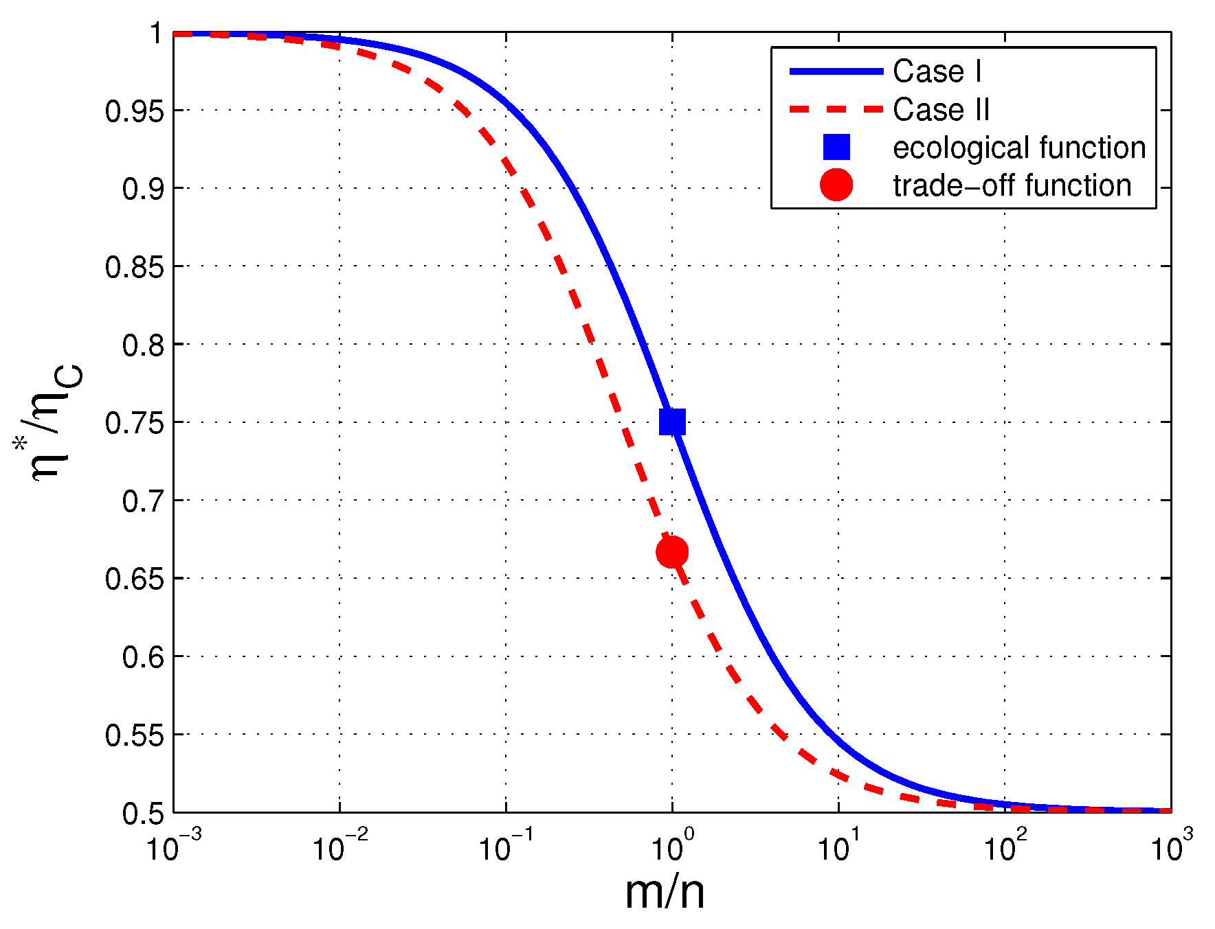
In Figure 1, we plot for Case I the rescaled efficiency ${\eta }^{*}/{\eta }_{\mathrm{C}}$ at the optimized objective function $F\left({\tau }^{*}\right)$ as a function of the ratio $m/n$ (solid line, with filled square indicating the result for the ecological function).

It is interesting to see three special cases:

• $m/n\to \infty$: To optimize F is essentially to optimize P. The optimized duration is ${\tau }^{*}=2\lambda$, and the corresponding efficiency is ${\eta }^{*}={\eta }_{\mathrm{C}}/2={\eta }_{\mathrm{VdB}}$, consistent with previous results [14]. In particular, the stopping time of the process is ${\tau }_{\mathrm{stop}}={\tau }^{*}/2=\lambda =\Phi /{\eta }_{\mathrm{C}}{Q}_{\mathrm{h}}$, whose physical meaning is clearly demonstrated that a process operated with such a duration will dissipate the amount of energy $\Phi /{\tau }_{\mathrm{stop}}$ that equals ${\eta }_{\mathrm{C}}{Q}_{\mathrm{h}}$; such a process does not output any work at all.
• $m/n\to 0$: To optimize F is essentially to minimize σ, and it is not surprising that we obtain a quasistatic process that takes ${\tau }^{*}\to \infty$ to finish, and the Carnot efficiency is naturally restored in this case, i.e., ${\eta }^{*}={\eta }_{\mathrm{C}}$.
• $m/n=1$: The objective function in this case is equivalent to the ecological function. The optimized duration is ${\tau }^{*}=4\lambda$, and the associated efficiency is $3{\eta }_{\mathrm{C}}/4$. These are also consistent with the previous results [8] to the first order of ${\eta }_{\mathrm{C}}$ (in the linear response regime).

4.2. Case II: $F=P^m{\eta }^n$

Similar to the case studied above, in order to optimize $F=P^m{\eta }^n$, we need to find the optimal duration ${\tau }^{*}$. Also note Equations (3) and (11), and $\eta =P/J_2$, we can see

$$\begin{array}{c}\hfill {\left(\frac{\partial F}{\partial q^2}\right)}_{J_2}=-T_{\mathrm{c}}(m+n)\frac{P^{m+n-1}}{J_2^n}{\left(\frac{\partial \sigma }{\partial q^2}\right)}_{J_2}>0.\end{array}$$

(24)

So F is also maximized when the tight-coupling condition $q^2=1$ is satisfied, and we can in this case rewrite F in terms of Φ and τ as

$$\begin{array}{c}\hfill F=\frac{{\left(\frac{{\eta }_{\mathrm{C}}{Q}_{\mathrm{h}}}{\tau }-\frac{\Phi }{{\tau }^2}\right)}^{m+n}}{{\left(\frac{{\eta }_{\mathrm{C}}{Q}_{\mathrm{h}}}{\tau }\right)}^n}.\end{array}$$

(25)

By letting $\partial F/\partial \tau =0$, we obtain the optimized duration ${\tau }^{*}$ as

$$\begin{array}{c}\hfill {\tau }^{*}=\frac{(2m+n)\lambda }{m},\end{array}$$

(26)

where $\lambda =\Phi /{\eta }_{\mathrm{C}}{Q}_{\mathrm{h}}$ as defined above. And the corresponding efficiency ${\eta }^{*}$ for maximized F is

$$\begin{array}{c}\hfill {\eta }^{*}={\eta }_{\mathrm{C}}\left(1-\frac{\lambda }{{\tau }^{*}}\right)=\frac{m+n}{2m+n}{\eta }_{\mathrm{C}}.\end{array}$$

(27)

In Figure 1, we also plot for Case II the rescaled efficiency ${\eta }^{*}/{\eta }_{\mathrm{C}}$ at the optimized objective function $F\left({\tau }^{*}\right)$ as a function of the ratio $m/n$ (dashed line, with filled circle denoting the result for the trade-off function).

There are also three special cases worth noting:

• $m/n\to \infty$: To optimize F is also essentially to optimize P. The optimized duration is ${\tau }^{*}=2\lambda$, and the corresponding efficiency is again ${\eta }^{*}={\eta }_{\mathrm{C}}/2={\eta }_{\mathrm{VdB}}$ [14]. With a stopping time ${\tau }_{\mathrm{stop}}=\lambda$, the process does not output any work.
• $m/n\to 0$: To optimize F is essentially to maximize η, or, equivalently, to minimize σ, and we obtain a quasistatic process that takes ${\tau }^{*}\to \infty$ to finish, and the Carnot efficiency is also restored in this case.
• $m/n=1$: The objective function in this case is equivalent to the trade-off function. The optimized duration is ${\tau }^{*}=3\lambda$, and the associated efficiency is $2{\eta }_{\mathrm{C}}/3$. These are also consistent with the previous results when the linear response regime is concerned [9].

4.3. Generic Cases

As for the generic cases, questions we are facing are: What kind of generic objective functions can we deal with in a unified way? Then, what results can we expect to be universally held for linear response? Note in either of the above two illustrative examples, the objective function is a function of P and σ or P and η, implying optimization is performed under some imposed constraints. In each case F is optimized when there is no direct heat leakage between two heat reservoirs, i.e., the optimization of F is achieved when the tight-coupling condition is satisfied. Under such a condition, Φ is helpful in the analysis of the optimization problem. In line with the above two cases, while from a broader perspective and an energy-saving point of view, we argue that a general F should at least satisfy

$$\begin{array}{c}\hfill {\left(\frac{\partial F}{\partial q^2}\right)}_{J_2}>0.\end{array}$$

(28)

We thus rule out objective functions that are optimized, for example, when the entropy production is maximized during a process. This requirement is actually consistent with Equation (18), but it is more physically meaningful, and one of its implications is: If it is possible to achieve the tight-coupling condition $q^2=1$, then a globally optimized F is expected, otherwise, we can consider the local optimal F under a given $q^2<1$. In the latter case, the corresponding optimized efficiency is generally less than that in the former case, because the heat leakage inevitably leads to the waste of heat flux and brings about extra entropy production. While if the tight-coupling condition can be fulfilled, then one can take advantage of Φ to solve for the optimized process whose corresponding efficiency serves as an upper bound for $q^2<1$: ${\eta }^{*}(q^2<1)<{\eta }^{*}(q^2=1)$. For simplicity, ${\eta }^{*}(q^2=1)$ is denoted ${\eta }^{*}$ throughout this work. As a result of the above reasoning, we know a unified approach to the optimization problems for linear response can be performed by taking advantage of Φ if the tight-coupling condition can be satisfied, and the resultant efficiency is a globally optimal one for reasonably chosen objective functions.

We have shown above how ${\eta }^{*}$ can be obtained for two specific choices of F. It is straightforward to adopt the same method to more generic situations as long as F is explicitly given. The procedures are: First, we rewrite F as a function of $J_2$ and σ with other parameters like $Q_{\mathrm{h}}$, $T_{\mathrm{h}}$, and $T_{\mathrm{c}}$ being prescribed or fixed. Then we replace $J_2$ by $Q_{\mathrm{h}}/\tau$, and $T_{\mathrm{c}}\sigma$ by $\Phi /{\tau }^2$, respectively. Note that now F is only a function of τ. By setting $\partial F/\partial \tau =0$, we obtain the optimized duration ${\tau }^{*}$. Finally, as for the corresponding efficiency ${\eta }^{*}$, we know that

$$\begin{array}{c}\hfill {\eta }^{*}=\frac{P\left({\tau }^{*}\right)}{J_2\left({\tau }^{*}\right)}=\frac{{\eta }_{\mathrm{C}}{J}_2\left({\tau }^{*}\right)-T_{\mathrm{c}}\sigma \left({\tau }^{*}\right)}{J_2\left({\tau }^{*}\right)}={\eta }_{\mathrm{C}}-\frac{\Phi /{\tau }^{*2}}{Q_{\mathrm{h}}/{\tau }^{*}}={\eta }_{\mathrm{C}}\left(1-\frac{\Phi }{{\eta }_{\mathrm{C}}{Q}_{\mathrm{h}}{\tau }^{*}}\right)={\eta }_{\mathrm{C}}\left(1-\frac{\lambda }{{\tau }^{*}}\right),\end{array}$$

(29)

as already shown in Equations (23) and (27). Note that the physical meaning of λ is the stopping time of the process, we thus have a formally universal result:

$$\begin{array}{c}\hfill {\eta }^{*}={\eta }_{\mathrm{C}}\left(1-\frac{{\tau }_{\mathrm{stop}}}{{\tau }^{*}}\right).\end{array}$$

(30)

This result physically clearly demonstrates how the efficiency of a desired process is related to the ratio between the stopping time of the process and the optimized duration. For a process with minimum entropy production, ${\tau }_{\mathrm{stop}}/{\tau }^{*}\to 0$, while for one with maximum power output, ${\tau }_{\mathrm{stop}}/{\tau }^{*}=1/2$. Since these two cases typically represent two extremes of optimization problems, generally the resultant ${\eta }^{*}$ lies in the range between ${\eta }_{\mathrm{C}}/2$ and ${\eta }_{\mathrm{C}}$. Equation (30) is thus one universal result that holds for reasonably chosen objective functions in the linear response regime. The universality of Equation (30) has two meanings: First, it is formally valid for various choices of reasonable objective functions F; second, as long as a specific F is chosen, different models or heat transfer laws will not alter ${\eta }^{*}$ in the linear response regime. The latter point is due to the generality of Onsager’s theory of linear irreversible thermodynamics. When F is chosen to be P, ${\eta }_{\mathrm{VdB}}$ is the universal efficiency, as already evidenced for various models [14,18,19]. Similarly, when F is generic, one can still expect a universal efficiency ${\eta }^{*}$ as given by Equation (30), irrespective of model details.

5. Conclusions

In this work, we show that within the framework of linear irreversible thermodynamics, there exists a lower bound of dissipation Φ (Equation (14)) for finite-time heat-work conversion processes, which is achieved when there is no direct heat leakage between two heat reservoirs and the tight-coupling condition is fulfilled. By taking advantage of Φ, we manage to optimize generic objective functions in a unified way. Two specific forms of objective functions are quantitatively analyzed, and a good agreement with previous results is obtained for either case in the linear response regime. For more general cases, we unveil a universal expression of efficiency for the optimized process (Equation (30)), in which the ratio between the stopping time and the optimized duration time of the process determines the corresponding efficiency. In a word, we present a unified approach to optimizing generic objective functions for linear response, and the corresponding efficiency is obtained universally.

Our work thus establishes a basis on which various thermodynamic processes can be treated in a simple and direct way. The results thus obtained are exact to the first order of ${\eta }_{\mathrm{C}}$, which provide a starting point for further investigations concerning model-dependent nonlinear response effects [26].