Generalized Einstein’s Equations from Wald Entropy

Abstract

We derive the gravitational equations of motion of general theories of gravity from thermodynamics applied to a local Rindler horizon through any point in spacetime. Specifically, for a given theory of gravity, we substitute the corresponding Wald entropy into the Clausius relation. Our approach works for all diffeomorphism-invariant theories of gravity in which the Lagrangian is a polynomial in the Riemann tensor.

1. Introduction

It has long been an attractive idea that gravity is not fundamental but, rather, emerges out of some more fundamental constituents. This concept dates back to Wheeler’s ideas on pre-geometry and to Sakharov’s proposal on induced gravity. A more modern version of this is the gauge/gravity duality of string theory in which gravity is described by a gauge theory that lives in one dimension less; since the gauge theory does not itself contain the spacetime metric as a fundamental dynamical field, from this point of view, gravity is emergent.

A great advance in the emergent gravity paradigm was made by Jacobson [1]. Jacobson considered the puzzling fact that the laws of black hole mechanics, derived in classical general relativity, seem mysteriously to anticipate the laws of black hole thermodynamics, derived in semi-classical gravity. Rather than trying to explain how classical laws could “know about” quantum-mechanical ones, Jacobson reversed the logic, regarding the thermodynamics to be a premise rather than a consequence. Quite remarkably, by assigning the thermodynamic properties of black hole horizons to local light-cones in spacetime (not necessarily near a black hole), the Einstein equation re-appears as an equation of state. This seems to suggest that gravity arises in some thermodynamic approximation through the coarse-graining of some underlying microscopics.

The question arises whether this alluring result is somehow an artifact of Einstein gravity, or whether the connection between thermodynamics and gravity goes deeper, persisting also in general, higher-curvature theories of gravity. But extending the original derivation to higher-curvature theories is nontrivial, in part because that derivation makes use of the Raychaudhuri equation, whose usefulness is obscured in higher-curvature theories: the Raychaudhuri equation relates the derivative of the expansion of the horizon to the Ricci tensor, but a simple relation between the Ricci tensor and the stress tensor holds only for Einstein gravity. Moreover, in generic theories of gravity, the entropy is not simply proportional to the area.

In this paper, we obtain the classical gravitational equations from thermodynamics without making use of the Raychaudhuri equation. Specifically, we show that the classical equations of gravity follow directly from the Clausius relation, $\delta \mathcal{S}=\delta Q/T$. Here for $\mathcal{S}$ we use Wald’s definition of entropy, which is the entropy (in place of $A/4$) that satisfies the first law of thermodynamics in higher-curvature theories. Our result suggests that classical gravitation always appears to have a quite intriguing thermodynamic origin. This provides support for the idea that gravity might be emergent; however, it should be clarified that the sense in which the word “emergent” is used in the gravitational literature is weaker than in condensed matter: no properties of the microscopic theory are invoked here, and the only place where coarse-graining is indicated is in the Planckian units in which geometric entropy is defined.

2. Results

2.1. General Theories of Gravity

Consider a general diffeomorphism-invariant theory of gravity in any number of dimensions. For simplicity and convenience, we will assume that the Lagrangian is a polynomial in the Riemann tensor but does not involve its derivatives. One may regard the Lagrangian formally as dependent on both the metric and the Riemann tensor even though of course the Riemann tensor depends on the metric [2,3]. Specifically, let the action be

$$I=\frac{1}{16\pi }\int d^{D}x\sqrt{-g}L(g_{ab},R_{abcd})+I_{\mathrm{matter}}.$$

(1)

We have set Newton’s constant to unity. Define

$$P^{abcd}={\displaystyle \frac{\partial L}{\partial R_{abcd}}}.$$

(2)

$P^{abcd}$ has the same algebraic symmetries as the Riemann tensor, including cyclicity. One then finds that the equation of motion that follows from Equation (1) (supplemented by appropriate generalizations of Gibbons-Hawking-like boundary terms and with minimal coupling to matter) is

$$P_a^{cde}{R}_{bcde}-2{\nabla }^c{\nabla }^d{P}_{acdb}-{\displaystyle \frac{1}{2}}L{g}_{ab}=8\pi T_{ab}.$$

(3)

For example, when the Lagrangian is $L=f\left(R\right)$, we find $P^{abcd}={\displaystyle \frac{1}{2}}{f}^{\prime }\left(R\right)\left(g^{ac}{g}^{bd}-g^{ad}{g}^{bc}\right)$. Thus, the equation of motion is

$$f^{\prime }\left(R\right)R_{ab}-{\nabla }_a{\nabla }_b{f}^{\prime }\left(R\right)+\left(\square f^{\prime }\left(R\right)-{\displaystyle \frac{1}{2}}f\left(R\right)\right)g_{ab}=8\pi T_{ab}.$$

(4)

This reduces to Einstein’s equation when $f\left(R\right)=R$.

Another example is Lovelock gravity [4,5], the most general extension of Einstein gravity for which the equations of motion do not contain derivatives of the Riemann tensor. The Lagrangian is $L={\sum }_{m=0}^{m_{\max }}{c}_m{L}_m$, where $c_m$ are constants of dimension ${(\mathrm{length})}^{2m-2}$, which are arbitrary as far as gravity is concerned, and $m_{\max }=(D-2)/2$ for even D dimensions and $m_{\max }=(D-1)/2$ for odd D. Each term $L_m$ is made up of contractions of products of the Riemann tensor:

$$L_m=\frac{1}{2^m}{\delta }_{j_1\dots j_{2m}}^{i_1\dots i_{2m}}{R^{j_1{j}_2}}_{i_1{i}_2}\dots {R^{j_{2m-1}{j}_{2m}}}_{i_{2m-1}{i}_{2m}}.$$

(5)

Here the δ symbol is the generalized Kronecker delta, defined as the sum over signed permutations of products of ordinary Kronecker deltas. The Einstein-Hilbert action with a cosmological constant is just a special case of the Lovelock action with $c_1=1$ and $c_0=-2\Lambda$. When $D\le 4$, there are no other possible terms; the next term appears for $D\ge 5$. It is $L_2=R^2-4R^{ab}{R}_{ab}+R^{abcd}{R}_{abcd}$, known as Gauss-Bonnet gravity, which appears in the low-energy effective action of certain string theories [6,7]; its coefficient in ten-dimensional heterotic string theory is $c_2=+{\alpha }^{\prime }/4$. The Gauss-Bonnet action is a topological invariant in four dimensions, just as the Einstein-Hilbert action is a topological invariant in two dimensions. It is convenient to write Equation (5) in the form [8]

$$L_m=Q_{\left(m\right)}^{abcd}{R}_{abcd}.$$

(6)

Then, for the mth-order Lovelock Lagrangian, $P^{abcd}=m{Q}_{\left(m\right)}^{abcd}$, which has the nice property that ${\nabla }_a{P}^{abcd}=0$. The equation of motion for Lovelock theory is therefore

$$\sum _{m=0}^{m_{\max }}{c}_m\left(m{Q}_{\left(m\right)}^{acde}{R}_{cde}^b-{\displaystyle \frac{1}{2}}{L}_m{g}^{ab}\right)=8\pi T^{ab},$$

(7)

which follows easily from Equation (3).

In each of these theories, one can associate an entropy with Killing or black hole horizons. For example, in place of $A/4$, the entropy in $f\left(R\right)$ gravity is [9]

$${\mathcal{S}}_f=f^{\prime }\left(R\right){\displaystyle \frac{A}{4}},$$

(8)

while for Einstein-Gauss-Bonnet gravity, black holes have an entropy of

$${\mathcal{S}}_{\mathrm{G}-\mathrm{B}}={\displaystyle \frac{1}{4}}\int d^{D-2}x\sqrt{\sigma }\left(1+2c_2{}^{(D-2)}R\right),$$

(9)

where ${}^{(D-2)}R$ is the scalar curvature of (the cross-section of) the horizon. We will show below that, as in Jacobson’s derivation of Einstein’s equation from $S=A/4$ [1], varying these entropies and imposing the Clausius relation, $\delta Q=T\delta S$, leads directly to the equations of classical gravity.

2.2. Wald Entropy

Wald [2,3] and other authors [10,11] have developed a powerful and elegant Lagrangian-based method for determining the entropy of a black hole with a Killing horizon. Wald’s method works for any diffeomorphism-invariant theory in any number of dimensions and does not require Euclideanization. Here we adopt a simplified version of the formalism [12]. Consider a generally covariant Lagrangian, L, that depends on the Riemann tensor but does not contain derivatives of the Riemann tensor.

Under the diffeomorphism $x^a\to x^a+{\xi }^a$ the metric changes via $\delta g_{ab}=-{\nabla }_a{\xi }_b-{\nabla }_b{\xi }_a$. By diffeomorphism-invariance, the change in the action, when evaluated on-shell, is given only by a surface term. This leads to a conservation law, ${\nabla }_a{J}^a=0$, for which we can write $J^a={\nabla }_b{J}^{ab}$, where $J^{ab}$ defines (not uniquely) the antisymmetric Noether potential associated with the diffeomorphism ${\xi }^a$ [2].

For a Lagrangian of the type $L=L(g_{ab},R_{abcd})$ direct computation shows that $J^{ab}$ is given by (see [12])

$$J^{ab}=-2P^{abcd}{\nabla }_c{\xi }_d+4{\xi }_d\left({\nabla }_c{P}^{abcd}\right),$$

(10)

with $P^{abcd}=\partial L/\partial R_{abcd}$. The Noether charge associated with a rigid diffeomorphism ${\xi }^a$ is defined by integrating the Noether potential over a closed spacelike surface S:

$$Q={\int }_S{J}^{ab}d{S}_{ab}.$$

(11)

When ${\xi }^a$ is a timelike Killing vector (the one whose norm vanishes at the Killing horizon), it turns out [2,3] that the corresponding Noether charge is precisely the entropy, $\mathcal{S}$, associated with the horizon, apart from a few factors:

$$\mathcal{S}={\displaystyle \frac{1}{8\kappa }}{\int }_{S}d{S}_{ab}{J}^{ab}.$$

(12)

Here κ is the surface gravity of the black hole horizon. The integral for this “Wald entropy” can be evaluated over any spacelike cross-section of the Killing horizon [10]. In fact we can formally define the quantity $\mathcal{S}$ on any closed spacelike surface, S, of codimension two (such as a section of a stretched horizon), and only at the end take the limit in which that S approaches a section of the Killing horizon. It can be shown, for example, that both Equation (8) and Equation (9) are just special cases of Wald entropy.

2.3. Gravitation From Thermodynamics

Now let us show how the classical equations of gravity, Equation (3), arise thermodynamically. (That the equations look thermodynamical has been shown for various special cases [13,14].) The set-up is as follows [1]. Take any spacetime point p and pick any future-directed null vector $k^a$ emanating from p. In the vicinity of p, the geometry is of course locally flat; this means that the metric is the Cartesian Minkowski metric to order $x^2$ when Taylor-expanded in Riemann normal coordinates centered at p. 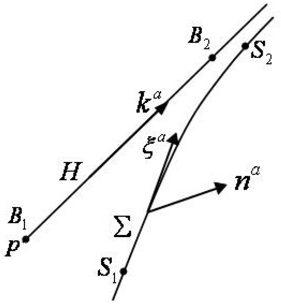The plane orthogonal to $k^a$ thus defines a local acceleration, or Rindler, horizon, H. Thus, in effect, we are drawing a “local" horizon through every point in spacetime. Let $B_1$ be any spacelike neighborhood of p of codimension two that lives on the Rindler plane, and let $B_2$ be some further section of the Rindler plane along $k^a$. Next, let ${\xi }^a$ be a future-directed timelike vector that generates boosts and asymptotically approaches $k^a$. For example, ${\xi }^a=x{\left({\displaystyle \frac{\partial }{\partial t}}\right)}^a+t{\left({\displaystyle \frac{\partial }{\partial x}}\right)}^a$. This would be a true Killing vector if the spacetime were flat. Generically, ${\xi }^a$ is an approximate Killing vector in that it satisfies Killing’s equation to order x in Riemann normal coordinates at p; we will always drop higher order terms below. A timelike congruence about ${\xi }^a$ then defines a stretched horizon, Σ. As in the membrane paradigm [15,16], points on H and points on Σ can be put in one-to-one correspondence by, say, ingoing null rays that pierce both surfaces. Let $S_i$ be the images of $B_i$ on Σ via this correspondence. See Figure 1.

Let ${\xi }^a{\xi }_a=-{\alpha }^2$, where the norm α (which is the lapse) is taken to be constant over Σ. This norm vanishes at H, a Killing horizon. Let $u^a$ be the proper velocity of a fiducial observer moving along the orbit of ${\xi }^a$i.e., $u^a={\left({\displaystyle \frac{d}{d\tau }}\right)}^a={\displaystyle \frac{1}{\alpha }}{\xi }^a$, where τ is the proper time. Let $n^a$ be the spacelike unit normal to Σ, pointing in the direction of increasing α. Both $u^a$ and $n^a$ map to $k^a$ in the limit that $\alpha \to 0$, for which $\Sigma \to H$.

After these preliminaries, we are ready to deduce the classical equations of gravity from thermodynamics. The key idea [1] is to assign black hole thermodynamic properties to local Rindler horizons. The stretched horizon can be assigned a local temperature, $T_{\mathrm{loc}}=\kappa /2\pi \alpha$, as well as the Wald entropy appropriate to the given theory of gravity; this means that the surface gravity, κ, is required to be approximately constant over Σ.

By Equation (10) and Equation (12), the Wald entropy associated with a compact section of the stretched horizon at time τ is

$$\mathcal{S}=-{\displaystyle \frac{1}{4\kappa }}{\int }_{S\left(\tau \right)}d{S}_{ab}\left(P^{abcd}{\nabla }_c{\xi }_d-2{\xi }_d{\nabla }_c{P}^{abcd}\right).$$

(13)

We now vary the entropy along the timelike congruence. Since the surface gravity is constant (to leading order) over Σ, κ can be taken outside the integral. Then the entropy change is

$$\begin{array}{ccc}\hfill \delta \mathcal{S}& =& \mathcal{S}\left({\tau }_2\right)-\mathcal{S}\left({\tau }_1\right)\hfill \\ & =& -{\displaystyle \frac{1}{4\kappa }}\left[{\int }_{S\left({\tau }_2\right)}d{S}_{ab}\left(P^{abcd}{\nabla }_c{\xi }_d-2{\xi }_d{\nabla }_c{P}^{abcd}\right)-{\int }_{S\left({\tau }_1\right)}d{S}_{ab}\left(P^{abcd}{\nabla }_c{\xi }_d-2{\xi }_d{\nabla }_c{P}^{abcd}\right)\right]\hfill \\ & =& +{\displaystyle \frac{1}{4\kappa }}{\int }_{\Sigma }d{\Sigma }_a{\nabla }_b\left(P^{abcd}{\nabla }_c{\xi }_d-2{\xi }_d{\nabla }_c{P}^{abcd}\right).\hfill \end{array}$$

(14)

In the last step, we have used Stokes’ theorem for an antisymmetric tensor field $A^{ab}$:

$$\begin{array}{c}\hfill {\int }_{\Sigma }d{\Sigma }_a{\nabla }_b{A}^{ab}=-\underset{\partial \Sigma }{\oint }d{S}_{ab}{A}^{ab},\end{array}$$

(15)

where the minus sign comes about because Σ is timelike. (To be explicit, our conventions here are $d{\Sigma }_a=n_{a}dAd\tau$ and $d{S}_{ab}={\displaystyle \frac{1}{2}}(n_a{u}_b-u_a{n}_b)dA$ on $S\left(\tau \right)$, where the normal $n^a$ to the stretched horizon points outwards, away from the true horizon.) Here we have discarded a surface term in Stokes’ theorem corresponding to the “vertical” boundaries joining the endpoints of $S\left({\tau }_2\right)$ and $S\left({\tau }_1\right)$; this can be justified by having the constant-time slices curve up so that $S\left({\tau }_1\right)$ and $S\left({\tau }_2\right)$ have common boundaries [17]. Next, recall that $P^{abcd}$ has the same algebraic symmetries as the Riemann tensor, including cyclicity. Using those symmetries, we find that

$$\delta \mathcal{S}={\displaystyle \frac{1}{4\kappa }}{\int }_{\Sigma }\left[-{\nabla }_b\left(P^{adbc}+P^{acbd}\right){\nabla }_c{\xi }_d+P^{abcd}{\nabla }_b{\nabla }_c{\xi }_d-2{\xi }_d{\nabla }_b{\nabla }_c{P}^{abcd}\right]d{\Sigma }_a.$$

(16)

Now we will use the fact that ${\xi }^a$ is an approximate timelike Killing vector, as defined earlier. Locally (to order x in Riemann normal coordinates), ${\xi }^a$ satisfies Killing’s equation. Hence the terms in parentheses drop out since they are symmetric in the indices c and d, whereas ${\nabla }_c{\xi }_d$ is antisymmetric. We will now assume the approximate validity of Killing’s identity, ${\nabla }_a{\nabla }_b{\xi }_c\approx R_{abc}^d{\xi }_d$, a point we discuss further in the next section. Then we find

$$T_{\mathrm{loc}}\delta \mathcal{S}={\displaystyle \frac{1}{8\pi \alpha }}{\int }_{\Sigma }\left(P^{abcd}{R}_{dcbe}{\xi }^e-2{\xi }_d{\nabla }_b{\nabla }_c{P}^{abcd}\right)n_{a}d\tau dA.$$

(17)

On the other hand, the locally-measured energy or heat flux into the stretched horizon is

$$\delta Q=+{\int }_{\Sigma }d{\Sigma }_a{T}_e^a{u}^e={\displaystyle \frac{1}{\alpha }}{\int }_{\Sigma }dAd\tau n_a{T}_e^a{\xi }^e.$$

(18)

Now we take the limit $\alpha \to 0$ in which the stretched horizon, Σ, becomes the true horizon, H. Then both $n^a$ and $u^a$ become proportional to the null vector $k^a$ (with the same proportionality constant). Writing $k^a={\left({\displaystyle \frac{d}{d\lambda }}\right)}^a$ where λ is some affine parameter, and equating $\delta Q$ and $T_{\mathrm{loc}}\delta \mathcal{S}$, we can show that

$${\int }_H\left(P_a^{cde}{R}_{bcde}-2{\nabla }^c{\nabla }^d{P}_{acdb}-8\pi T_{ab}\right)k^a{k}^{b}d\lambda dA=0.$$

(19)

As this holds for any p and any null $k^a$, the integral does not depend on the domain, so the integrand must be zero, up to a term that vanishes when contracted with $k^a{k}^b$:

$$P_a^{cde}{R}_{bcde}-2{\nabla }^c{\nabla }^d{P}_{acdb}+\phi g_{ab}=8\pi T_{ab},$$

(20)

for some scalar function $\phi$. By demanding conservation of the stress tensor and using the Bianchi identities, we find that $\phi =-{\displaystyle \frac{1}{2}}L+\Lambda$, where Λ is an integration constant. Thus we see that imposing $T_{\mathrm{loc}}\delta \mathcal{S}=\delta Q$ at any point in spacetime necessarily implies that

$$P_a^{cde}{R}_{bcde}-2{\nabla }^c{\nabla }^d{P}_{acdb}-{\displaystyle \frac{1}{2}}L{g}_{ab}+\Lambda g_{ab}=8\pi T_{ab}.$$

(21)

With the cosmological constant appearing as an integration constant, this is precisely the classical equation of motion, Equation (3), for our theory of gravity.

3. Discussions

We have shown that the equations of classical gravity follow from thermodynamics. Our derivation did not require the Raychaudhuri equation. Moreover, since we started with the Wald entropy, we could go beyond the Einstein equation to the equations of motion of general theories of gravity. Since these were obtained from the Clausius relation, they can be regarded as equations of state—relations between thermodynamic state variables. Thus it seems as though classical gravity has a thermodynamic origin and, furthermore, that this relation between gravity and thermodynamics extends beyond Einsteinian gravity. Moreover, our approach suggests why such a relation exists: both the Wald entropy and the equations of motion are ultimately derived from an action. In Jacobson’s original calculation, the relation to the action was not apparent, making the result appear mysterious, but such a relation was nevertheless present since the Bekenstein-Hawking entropy that was used there is simply a special case of the Wald entropy.

A technical point we have glossed over is the use of the equation ${\nabla }_a{\nabla }_b{\xi }_c\approx R_{abcd}{\xi }^d$ in Equation (17), an expression that is strictly true only when ${\xi }^a$ is an exact Killing vector. Killing’s identity is of order x and therefore is of the same order as the terms we would like to keep. Fortunately, it can be shown that, by appropriately defining higher order terms in ${\xi }^a$, the identity can be made to hold in the vicinity of a null geodesic. Therefore, by making the patch of Rindler space sufficiently narrow, Killing’s identity can be assumed throughout the calculation [17].

It would also be interesting to connect our approach to previous calculations, which have had a quite different methodology. For example, for $f\left(R\right)$ theories, previous work has found that the Clausius relation does not yield purely the equations of motion but also gives rise to additional terms [18]; these have been interpreted as non-equilibrium effects. However, there have also been claims [19] that the $f\left(R\right)$ equations of motion do follow from the Clausius relation, as we also find; indeed, the derivation in [19] also invokes the Wald entropy, though restricted to the case of $f\left(R\right)$ gravity. However, $f\left(R\right)$ gravity is a very special case and is closely related to Einstein gravity; therefore, the study of $f\left(R\right)$ gravity does not necessarily make clear what aspect of the derivation causes it to work. Here we have seen that the derivation works for a wide class of theories for which the Lagrangian is a polynomial in the Riemann tensor.

So far in the literature, derivations of the gravitational equations have taken place in the context of planar local Rindler horizons. But, as we know from black holes, horizons can also have spherical topology. It would be interesting therefore to derive the gravitational equations in a local formulation that mimics black hole horizons. For example, instead of the Killing vector ${\xi }^a=x{\left({\displaystyle \frac{\partial }{\partial t}}\right)}^a+t{\left({\displaystyle \frac{\partial }{\partial x}}\right)}^a$, one could work with radial vectors ${\xi }^a=r{\left({\displaystyle \frac{\partial }{\partial t}}\right)}^a+t{\left({\displaystyle \frac{\partial }{\partial r}}\right)}^a$. These, too, of course have constant acceleration. A family of such vectors at constant ${\xi }^2=-{\alpha }^2$ would trace out a de Sitter hyperboloid about the origin. Constant-time sections on such surfaces would be compact and therefore the issue of extra surface terms in Stokes’ theorem would not arise. Of course, Killing’s identity, which we also needed for our derivation, would not hold throughout such a surface, but perhaps its’ integral might nevertheless be made to vanish. We hope to pursue this approach in the future.

Satisfying as our result is, one possible critique of this program is that the derivation of the Wald entropy itself relies on the equations of motion being obeyed. Although our approach never explicitly invokes the equations of motion, it is somewhat unclear whether any derivation, including Jacobson’s original calculation, that begins with an on-shell expression which agrees with Wald entropy (such as $A/4$) is implicitly assuming the answer, or whether that is simply a consequence of self-consistency. In any case, ultimately one would like to obtain gravity as the thermodynamic limit of the statistical mechanics of some microscopic theory. Many diffeomorphism-invariant theories of gravity have pathologies, such as problems with unitarity, and these presumably do not have consistent microscopics. Entropy, after all, should satisfy not only the first law, but also have other expected properties: it should obey the second law, be non-negative, and have a statistical interpretation. Ideally, one would like to have a consistent dual theory without gravity, for which one can obtain the entropy by enumerating the microstates, and then, after expressing the entropy in geometric language, to obtain the dynamical equations of classical gravity from a thermodynamic limit, as described here. Some of this is of course reminiscent of what happens in several contexts in string theory.