
Statistical Evidence Measured on a Properly Calibrated Scale for Multinomial Hypothesis Comparisons

Abstract
:
1. Introduction
“To a certain degree this scheme is typical for all theoretic knowledge: We begin with some general but vague principle, then find an important case where we can give that notion a concrete precise meaning, and from that case we gradually rise again to generality and if we are lucky we end up with an idea no less universal than the one from which we started. Gone may be much of its emotional appeal, but it has the same or even greater unifying power in the realm of thought and is exact instead of vague.”([8], p. 6, emphasis added)
2. A Vague but General Understanding of Statistical Evidence
- (i)
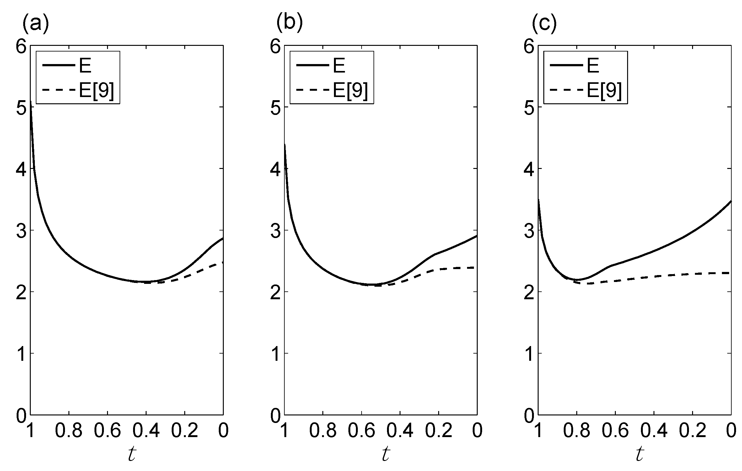
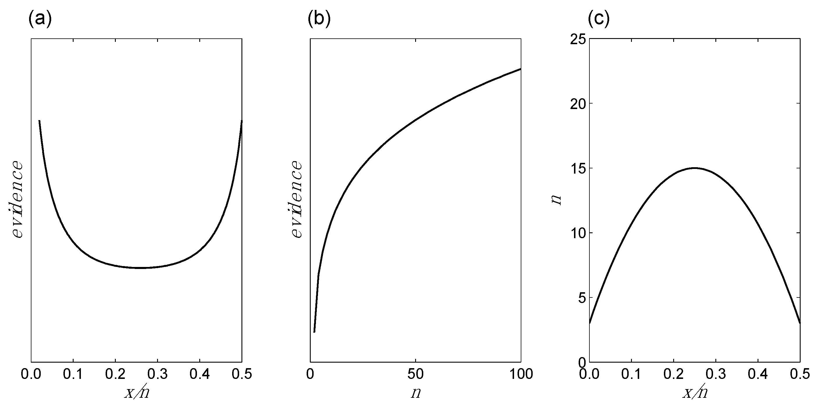
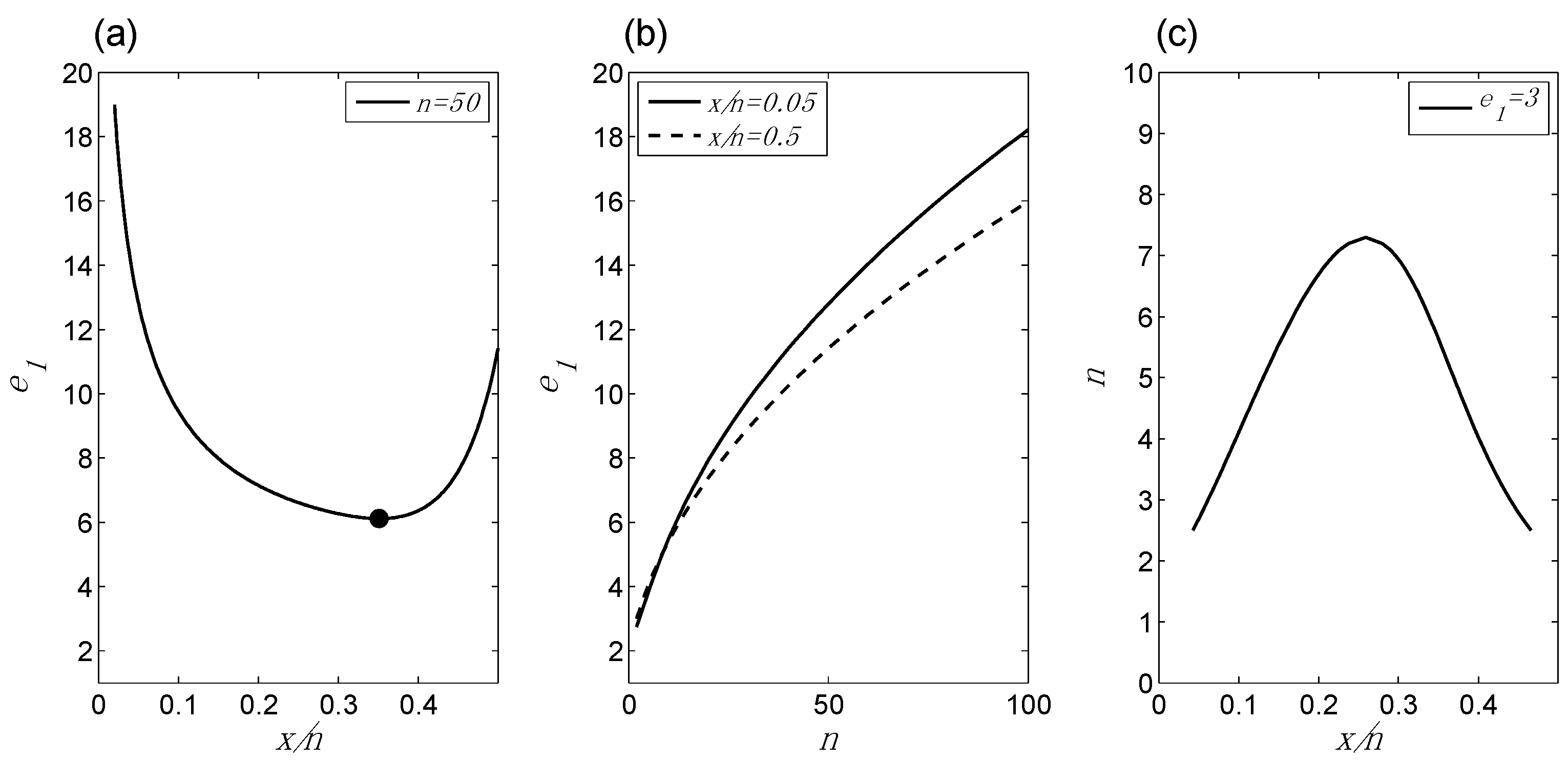
- Evidence as a function of changes in x/n for fixed n: If we hold n constant but allow x/n to increase from 0 up to ½, the evidence in favor of bias will at first diminish, and then at some point the evidence will begin to increase, as it shifts to favoring no bias. BBP(i) is illustrated in Figure 1a.
- (ii)
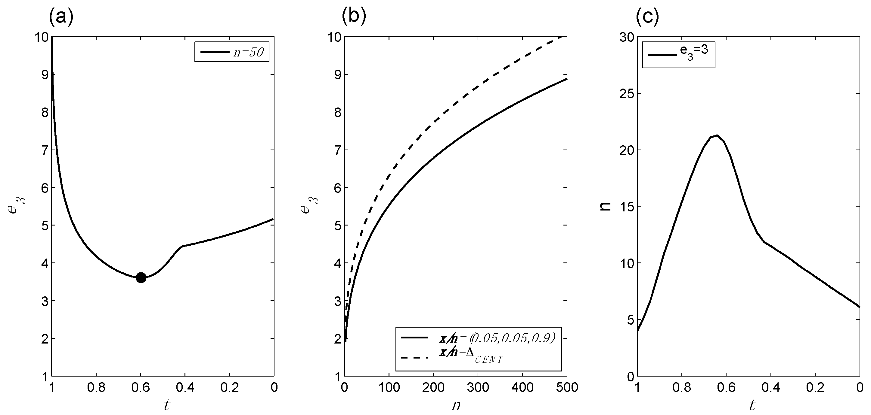
- Evidence as a function of changes in n for fixed x/n: For any given value of x/n, the evidence increases as n increases. The evidence may favor bias (e.g., if x/n = 0) or no bias (e.g., if x/n = ½), but in either case it increases with increasing n. Additionally, this increase in the evidence becomes smaller as n increases. For example, five tails in a row increase the evidence for bias by a greater amount if they are preceded by two tails, compared to if they are preceded by 100 tails. BBP(ii) is illustrated in Figure 1b.
- (iii)
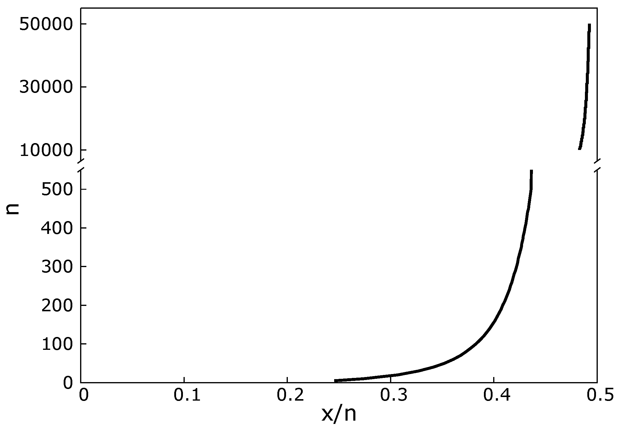
- x/n as a function of changes in n (or vice versa) for fixed evidence: It follows from BBPs(i) and BBPs(ii) that in order for the evidence to remain constant, n and x/n must adjust to one another in a compensatory manner. For instance, if x/n increases from 0 to 0.05, in order for the evidence to remain the same, n must increase to compensate; otherwise, the evidence would go down following BBP(i). BBP(iii) is illustrated in Figure 1c.
3. A Precise but Non-general Definition of Statistical Evidence
4. First Generalization: From e1 to e2
5. Second Generalization: From e2 to e3
6. Measurement Calibration
7. Discussion
“[There is] a notable dissimilarity between thermodynamics and the other branches of classical science….[Thermodynamics] reflects a commonality or universal feature of all laws…[it] is the study of the restrictions on the possible properties of matter that follow from the symmetry properties of the fundamental laws of physics. Thermodynamics inherits its universality…from its symmetry parentage.”([24], pp. 2–3)
Acknowledgments
Author Contributions
Conflicts of Interest
Abbreviations
| LR | Likelihood Ratio |
| BF | Bayes Factor |
| MLR | Maximum LR |
| ALR | Area under LR |
| VLR | Volume under LR |
| BBP | Basic Behavior Pattern (for evidence) |
| HC | Hypothesis Contrast |
| TrP | Transition Point |
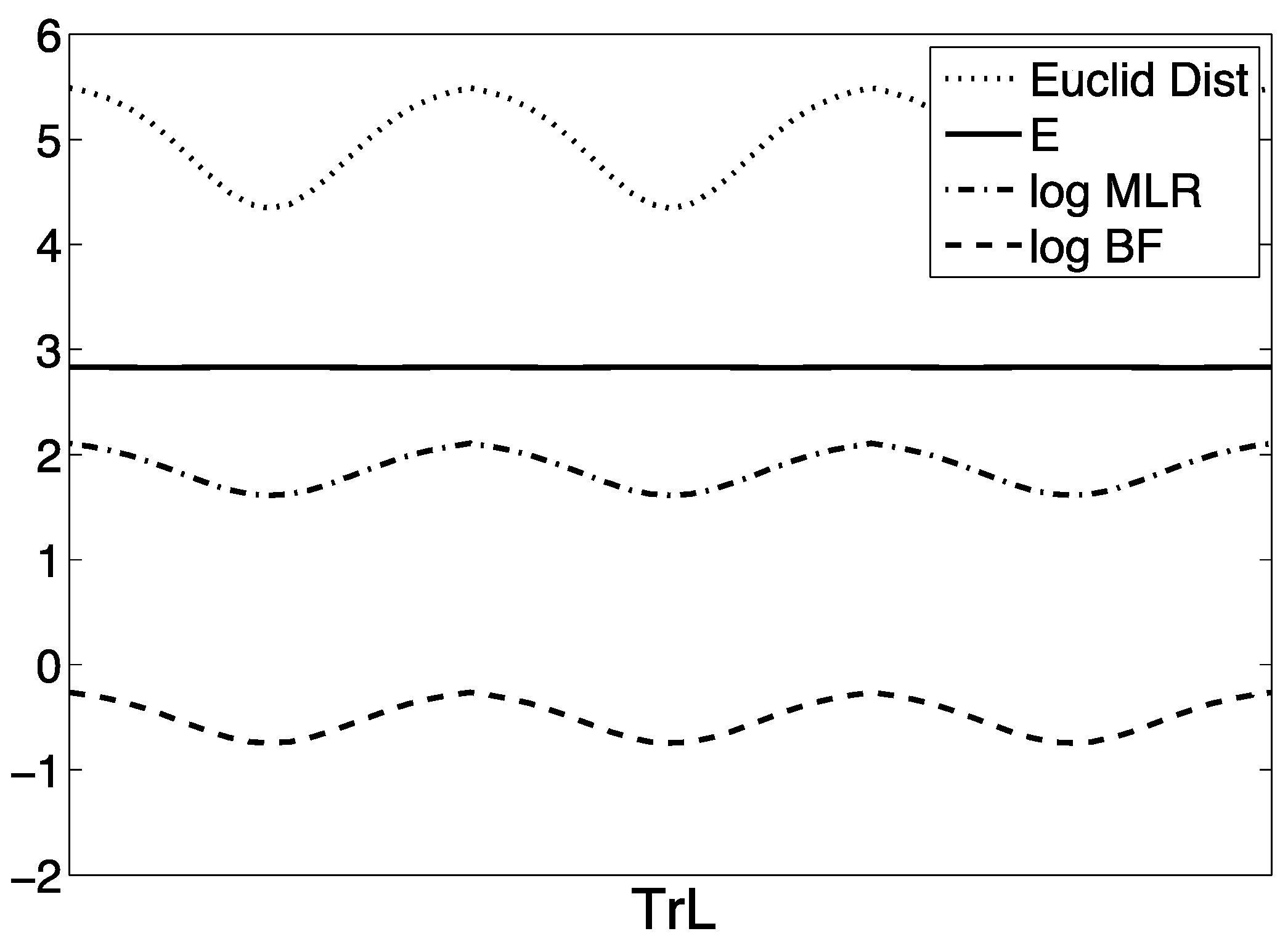
| TrL | Transition Line |
| TrPL | Transition Plane |
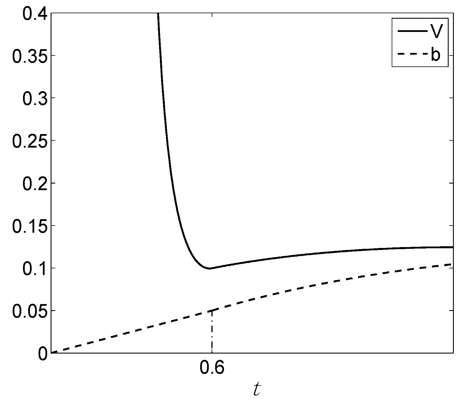
Appendix A. The constants d.f. and b


| m = 3 | m = 4 | |||||||
|---|---|---|---|---|---|---|---|---|
| n | Max E | Min E | Diff | Ratio | Max E | Min E | Diff | Ratio |
| 50 | 3.6510 | 3.6449 | 0.0061 | 0.0017 | 4.6245 | 4.6147 | 0.0098 | 0.0021 |
| 100 | 4.4949 | 4.4896 | 0.0053 | 0.0012 | 5.8440 | 5.8342 | 0.0098 | 0.0017 |
| 500 | 7.5096 | 7.5077 | 0.0019 | 0.0003 | 10.4134 | 10.4094 | 0.0040 | 0.0004 |
References
- Evans, M. Measuring Statistical Evidence Using Relative Belief (Monographs on Statistics and Applied Probability); CRC Press: Boca Raton, FL, USA, 2015. [Google Scholar]
- Hacking, I. Logic of Statistical Inference; Cambridge University Press: London, UK, 1965. [Google Scholar]
- Edwards, A. Likelihood; Johns Hopkins University Press: Baltimore, MD, USA, 1992. [Google Scholar]
- Royall, R. Statistical Evidence: A Likelihood Paradigm; Chapman & Hall: London, UK, 1997. [Google Scholar]
- Vieland, V.J. Thermometers: Something for statistical geneticists to think about. Hum. Hered. 2006, 61, 144–156. [Google Scholar] [CrossRef] [PubMed]
- Vieland, V.J. Where’s the Evidence? Hum. Hered. 2011, 71, 59–66. [Google Scholar] [CrossRef] [PubMed]
- Vieland, V.J.; Hodge, S.E. Measurement of Evidence and Evidence of Measurement. Stat. App. Genet. Molec. Biol. 2011, 10. [Google Scholar] [CrossRef]
- Weyl, H. Symmetry; Princeton University Press: Princeton, NJ, USA, 1952. [Google Scholar]
- Vieland, V.J.; Seok, S.-C. Statistical Evidence Measured on a Properly Calibrated Scale across Nested and Non-nested Hypothesis Comparisons. Entropy 2015, 17, 5333–5352. [Google Scholar] [CrossRef]
- Vieland, V.J.; Das, J.; Hodge, S.E.; Seok, S.-C. Measurement of statistical evidence on an absolute scale following thermodynamic principles. Theory Biosci. 2013, 132, 181–194. [Google Scholar] [CrossRef] [PubMed]
- Bickel, D.R. The strength of statistical evidence for composite hypotheses: Inference to the best explanation. Available online: http://biostats.bepress.com/cobra/art71/ (accessed on 24 March 2016).
- Zhang, Z. A law of likelihood for composite hypotheses. Available online: http://arxiv.org/abs/0901.0463 (accessed on 24 March 2016).
- Jeffreys, H. Theory of Probability (The International Series of Monographs on Physics); The Clarendon Press: Oxford, UK, 1939. [Google Scholar]
- Kass, R.E.; Raftery, A.E. Bayes Factors. J. Am. Stat. Assoc. 1995, 90, 773–795. [Google Scholar] [CrossRef]
- Fermi, E. Thermodynamics; Dover Publications: New York, NY, USA, 1956. [Google Scholar]
- Stern, J.M.; Pereira, C.A.D.B. Bayesian epistemic values: Focus on surprise, measure probability! Logic J. IGPL 2014, 22, 236–254. [Google Scholar] [CrossRef]
- Borges, W.; Stern, J. The rules of logic composition for the bayesian epistemic e-values. Logic J. IGPL 2007, 15, 401–420. [Google Scholar] [CrossRef]
- Kullback, S. Information Theory and Statistics; Dover Publications: Mineola, NY, USA, 1968. [Google Scholar]
- Vieland, V.J. Evidence, temperature, and the laws of thermodynamics. Hum. Hered. 2014, 78, 153–163. [Google Scholar] [CrossRef] [PubMed]
- Landauer, R. Irreversibility and heat generation in the computing process. IBM J. Res. Dev. 1961, 5, 183–191. [Google Scholar] [CrossRef]
- Jaynes, E.T. Information Theory and Statistical Mechanics. Phys. Rev. 1957, 106, 620–630. [Google Scholar] [CrossRef]
- Duncan, T.L.; Semura, J.S. The deep physics behind the second law: Information and energy as independent forms of bookkeeping. Entropy 2004, 6, 21–29. [Google Scholar] [CrossRef]
- Caticha, A. Relative Entropy and Inductive Inference. Available online: http://arxiv.org/abs/physics/0311093 (accessed on 24 March 2016).
- Callen, H.B. Thermodynamics and an Introduction to Thermostatistics, 2nd ed.; John Wiley & Sons: New York, NY, USA, 1985. [Google Scholar]


© 2016 by the authors; licensee MDPI, Basel, Switzerland. This article is an open access article distributed under the terms and conditions of the Creative Commons by Attribution (CC-BY) license (http://creativecommons.org/licenses/by/4.0/).
Share and Cite
Vieland, V.J.; Seok, S.-C. Statistical Evidence Measured on a Properly Calibrated Scale for Multinomial Hypothesis Comparisons. Entropy 2016, 18, 114. https://doi.org/10.3390/e18040114
Vieland VJ, Seok S-C. Statistical Evidence Measured on a Properly Calibrated Scale for Multinomial Hypothesis Comparisons. Entropy. 2016; 18(4):114. https://doi.org/10.3390/e18040114
Chicago/Turabian StyleVieland, Veronica J., and Sang-Cheol Seok. 2016. "Statistical Evidence Measured on a Properly Calibrated Scale for Multinomial Hypothesis Comparisons" Entropy 18, no. 4: 114. https://doi.org/10.3390/e18040114
APA StyleVieland, V. J., & Seok, S.-C. (2016). Statistical Evidence Measured on a Properly Calibrated Scale for Multinomial Hypothesis Comparisons. Entropy, 18(4), 114. https://doi.org/10.3390/e18040114