Application of Sample Entropy Based LMD-TFPF De-Noising Algorithm for the Gear Transmission System

Abstract

This paper investigates an improved noise reduction method and its application on gearbox vibration signal de-noising. A hybrid de-noising algorithm based on local mean decomposition (LMD), sample entropy (SE), and time-frequency peak filtering (TFPF) is proposed. TFPF is a classical filter method in the time-frequency domain. However, there is a contradiction in TFPF, i.e., a good preservation for signal amplitude, but poor random noise reduction results might be obtained by selecting a short window length, whereas a serious attenuation for signal amplitude, but effective random noise reduction might be obtained by selecting a long window length. In order to make a good tradeoff between valid signal amplitude preservation and random noise reduction, LMD and SE are adopted to improve TFPF. Firstly, the original signal is decomposed into PFs by LMD, and the SE value of each product function (PF) is calculated in order to classify the numerous PFs into the useful component, mixed component, and the noise component; then short-window TFPF is employed for the useful component, long-window TFPF is employed for the mixed component, and the noise component is removed; finally, the final signal is obtained after reconstruction. The gearbox vibration signals are employed to verify the proposed algorithm, and the comparison results show that the proposed SE-LMD-TFPF has the best de-noising results compared to traditional wavelet and TFPF method.

1. Introduction

A gear transmission is the basic form of mechanical transmission, so the gear system is an important component of mechanical systems which have been widely used in machine tools, vehicles, construction machinery, and other equipment [1,2]. The running state of the gear system is directly related to the entire mechanical equipment. Due to the reasons of complex structure and poor working conditions, the gear system is very prone to breakage, damage, and other faults. Therefore, the failure analysis and fault diagnosis of the gear system are important research areas and many signal processing methods have been developed [3,4]. However, signal noise greatly influences the failure analysis and fault diagnosis, which has attracted popularity to the research on noise reduction for gear systems [5,6] and many excellent achievements have been reported [7,8].

Many studies about noise reduction for gear systems have been carried out. The standard approach for extracting useful signals from a noisy background is designing an appropriate filter, which removes the noise components, and then the desired signal components are obtained. Recently, time-frequency analysis [9,10,11], such as wavelet transform (WT), empirical mode decomposition (EMD), and local mean decomposition (LMD), have become the well-accepted techniques, for they can provide both time and frequency domain information of the signal simultaneously. Wavelet transform has a multi-scale feature, which can provide local features in both time and frequency domains, enabling wavelet analysis to distinguish the abrupt components of the vibration signal [12]. This is the reason why wavelet transform has been widely used in rotating machinery fault diagnosis [13]. The wavelet transform method has the advantage of excellent time-frequency localization particularly, however, the appropriate choices of the wavelet base function or the certain frequency bands with fault information need to be solved. Empirical mode decomposition (EMD) is a self-adaptive signal processing method which can decompose a complex signal into intrinsic mode functions (IMFs) whose instantaneous frequencies have physical meaning. EMD has been widely used in machinery fault diagnosis since it was developed. However, many deficiencies in EMD still exist, such as end effects [14], IMF criterion [15], mode mixing [16], and so on. Local mean decomposition (LMD) was put forward by Jonathan S. Smith recently and has been widely used to analyze electroencephalogram signals. LMD is a self-adaptive time-frequency analysis method, which can self-adaptively decompose a complex signal into a set of product functions (PFs) [17]. Moreover, the comparison between the two adaptive methods EMD and LMD can be found in [18], which show that LMD is superior to the EMD method in many aspects. Therefore, the LMD technique has been further investigated than EMD to preprocess the vibration signals.

In addition to the time-frequency analysis methods, there are many other excellent de-noising methods. For example, forward linear prediction (FLP) is an effective de-nosing algorithm which has been successfully used to reduce the noise of fiber optic gyroscopes [19,20]. The time-frequency peak filtering (TFPF) technique is another effective random noise reduction method and has been applied to reduce seismic random noise effectively [21,22,23]. However, there exists a contradiction in TFPF; that is, when a short window length is selected, a good preservation for valid signal amplitude, but poor random noise reduction might result, whereas when a long window length is selected, a serious attenuation for signal amplitude, but effective random noise reduction might be obtained. Moreover, some researchers have proposed hybrid filters based on the advantages of single filters, such as the combination of EMD and TFPF [24], the EMD and non-local mean de-noising algorithm [25], the EMD and forward linear prediction filter [26], etc., and the experimental results show that the performance of hybrid filters tend to be improved because of the combined advantages.

For gear transmission system, vibration signals of different fault locations and different degrees of failures will show varying complexity, so various PFs obtained by LMD will increase the computation cost of hybrid filters. In order to simplify the computation process, Entropy is proposed to calculate the similarity of various PFs, and then the PFs will be classified according to the calculated similarity. Entropy has been widely and successfully used in signal processing due to sample entropy (SE) highlighting the simplicity, robustness, and reduced computational cost [27]. Due to the good performance in real-time, SE has been widely investigated and used in many research areas [28,29]. Therefore, SE is employed to calculate the similarity of various PEs in this paper.

In this paper, comprehensively considering the features of different de-noising algorithms, a hybrid noise reduction algorithm based on LMD, SE, and TFPF is proposed and the vibration signal measured from a gearbox is used to validate the proposed algorithm. The rest of the paper is organized as follows: Section 2 is the description of the proposed SE-LMD-TFPF algorithm; the experimental and results are shown in Section 3; and Section 4 is the conclusion.

2. Description of SE-LMD-TFPF

2.1. Local Mean Decomposition

LMD can be used to decompose complicated signals into a set of PF components. Each PF is the product of a frequency modulated (FM) signal and an envelope signal. The process of decomposition for any non-stationary signal is shown as follows:

● Step 1: Find all of the local extreme points $n_i$ of the original signal and calculate the local mean $m_i$:

$$m_i=\frac{n_i+n_{i+1}}{2}$$

(1)

The straight lines are used to connect the two points adjacent to each $m_i$. The local mean function $m_{11}\left(t\right)$ can be obtained by applying a moving average to smooth $m_i$.

● Step 2: Calculate the envelope estimation function $a_{11}\left(t\right)$:

$$a_i=\frac{\left|n_i-n_{i+1}\right|}{2}$$

(2)

Smooth the local envelope estimates $a_i$ in the same manner as the local means to obtain the envelope estimation function $a_{11}\left(t\right)$.

● Step 3: Calculate the FM signal $s_{11}\left(t\right)$:

$$h_{11}\left(t\right)=X\left(t\right)-m_{11}\left(t\right)$$

(3)

where $X\left(t\right)$ is the original signal. In order to demodulate $h_{11}\left(t\right)$, divide $h_{11}\left(t\right)$ by $a_{11}\left(t\right)$ to obtain:

$$s_{11}\left(t\right)=\frac{h_{11}\left(t\right)}{a_{11}\left(t\right)}$$

(4)

Ideally, $s_{11}\left(t\right)$ must be a pure FM signal. However, this condition is not always completely satisfied in reality. Considering the effects of decomposition, speed, and other factors, the conditions for the termination of the iteration process are given by:

$$a_{1n}\left(t\right)\approx 1$$

(5)

● Step 4: When $s_{1n}\left(t\right)$ satisfies the condition of being a pure FM signal, the corresponding envelop is given by:

$$a_1\left(t\right)=a_{11}\left(t\right)a_{12}\left(t\right)\cdots a_{1n}\left(t\right)={\displaystyle \prod }_{q=1}^n{a}_{1q}\left(t\right)$$

(6)

where q stands for the number of iteration loops. A single component of the AM-FM signal $P{F}_1\left(t\right)$ is given by:

$$P{F}_1\left(t\right)=a_1\left(t\right)s_{1n}\left(t\right)$$

(7)

● Step 5: Subtract the first PF component $P{F}_1\left(t\right)$ from the signal X(t) to obtain a new signal $u_1\left(t\right)$. Repeat the above step k times using $u_1\left(t\right)$ as the new source data until $u_k\left(t\right)$ becomes a monotonic function:

$$\{\begin{array}{c}{u}_1\left(t\right)=x\left(t\right)-P{F}_1\left(t\right)\hfill \\ u_2\left(t\right)=u_1\left(t\right)-P{F}_2\left(t\right)\hfill \\ \hfill \cdots \cdots \cdots \hfill \\ u_k\left(t\right)=u_{k-1}\left(t\right)-P{F}_k\left(t\right)\hfill \end{array}$$

(8)

Therefore, X(t) can be decomposed into a sum of PF components and $u_k\left(t\right)$:

$$X\left(t\right)={\displaystyle \sum }_{p=1}^{k}P{F}_P\left(t\right)+u_k\left(t\right)$$

(9)

2.2. Sample Entropy

After decomposition by LMD, the original signal will be decomposed into numerous PFs. Normally, there are many PFs that will be obtained. If we can classify the numerous PFs into limited kinds of components, the de-noising process will be more clear and pointed. Therefore, the sample entropy (SE) is introduced. SE examines the time series (here are the PFs) for similar epochs and assigns a non-negative number to the sequence, with larger values corresponding to more complexity or irregularity in the data.

SE can be calculated as follows [17]:

$$\mathrm{SE}\left(m,r,N\right)=ln\left[\frac{1}{N-m+1}{\displaystyle \sum }_{i=1}^{N-m+1}{C}_r^m\left(i\right)-\frac{1}{N-\left(m+1\right)+1}{\displaystyle \sum }_{i=1}^{N-\left(m+1\right)+1}{C}_r^{m+1}\left(i\right)\right]$$

(10)

where N is the length of signals, m is the match of length, and $C_r^m\left(i\right)$ is the probability that any two epochs match each other. By choosing a proper noise filter parameter r (usually chosen around 25% of the standard deviation of the signal) it is possible eliminate the effect of noise.

2.3. Basic Principle of TFPF

Gear system signals can often be considered as band-limited non-stationary deterministic signals which can be modeled by Equation (11):

$$y\left(n\right)=x\left(n\right)+r\left(n\right)$$

(11)

where, $x\left(n\right)$ is the pure gear signal components; $r\left(n\right)$ is the additive random noise, and $n$ is the sampling point. The noisy signal $y\left(n\right)$ is encoded by frequency modulation as instantaneous frequency of a unit amplitude analytic signal so as to actualize TFPF, which can be defined as Equation (12):

$$z_y\left(n\right){=\mathrm{e}}^{j2\pi \rho {\displaystyle \sum _{m=0}^{n}y\left(m\right)}}$$

(12)

where, $\rho$ is a scaling parameter analogous to the frequency modulation index. After frequency modulation and encoding, the noisy signal $y\left(n\right)$ is converted into the instantaneous frequency of the analytic signal $z_y\left(n\right)$.

Then, the recovered signal can be obtained as Equation (13) by estimating the peak in the frequency of pseudo Wigner–Ville distribution of $z_y\left(n\right)$:

$${\stackrel{\wedge }{x}}_h\left(n\right)=f_z\left(n\right)=\frac{\underset{f}{\arg \max \left[P{W}_z\left(n,f\right)\right]}}{\rho }$$

(13)

where, $P{W}_z\left(n, f\right)$ represents the pseudo Wigner–Ville distribution of $z_y\left(n\right)$ and the pseudo Wigner–Ville distribution with time-varying window $h\left(m\right)$ is defined as:

$$P{W}_z\left(n,f\right)={\displaystyle \sum _{m=-\infty }^{\infty }h\left(m\right)}\overline{z_y}\left(n-m\right)z_y\left(n+m\right)e^{-j4\pi fm}$$

(14)

where, $\overline{z_y}$ is the conjugate operator to $z_y$. The length of the window function $h\left(m\right)$ is a trade-off parameter for random noise attenuation and signal preservation.

2.4. Steps of SE-LMD-TFPF

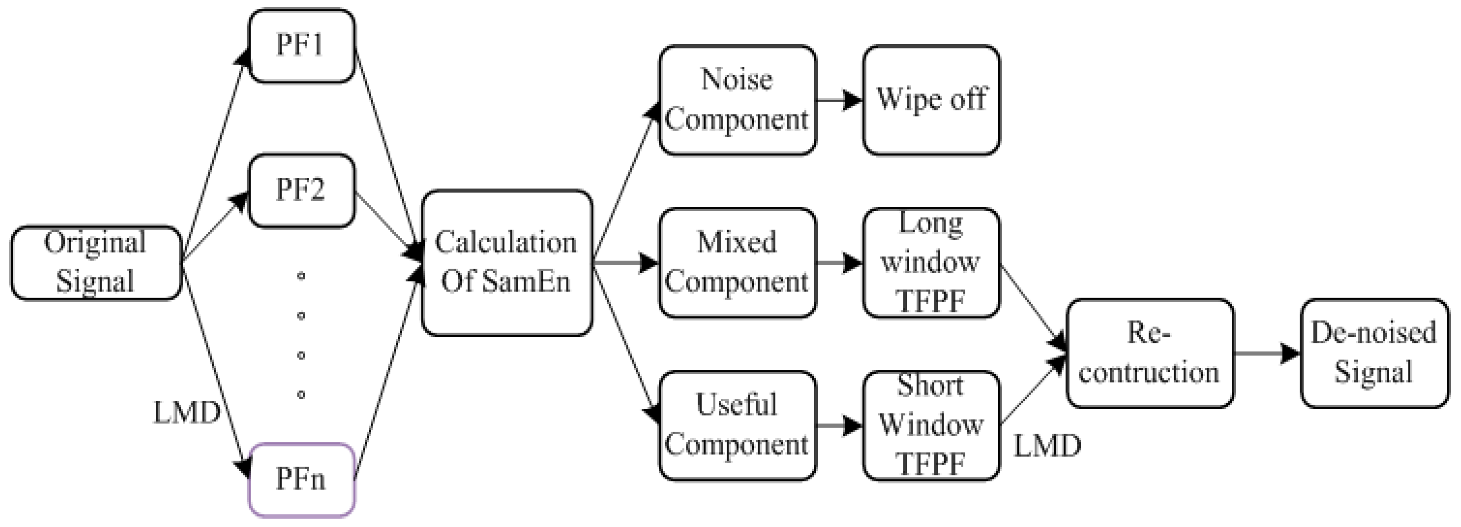
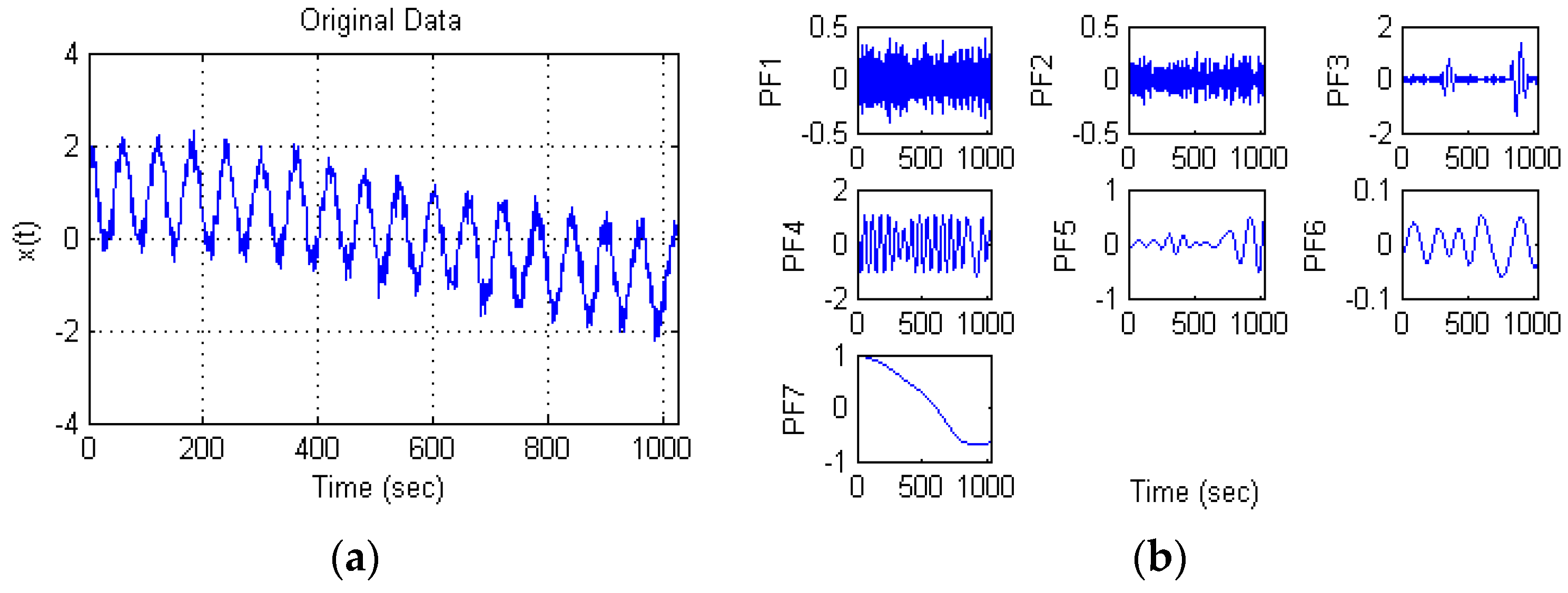
In order to combine the advantages of LMD and TFPF, the hybrid noise reduction algorithm SE-LMD-TFPF is proposed. There are four steps of the proposed SE-LMD-TFPF algorithm as shown in Figure 1. A simulated signal $x(t)$ is employed to explain the step by step working principle of the SE-LMD-TFPF algorithm, where t is time and $\phi (t)$ is the added Gaussian white noise:

$$x(t)=\cos (2\pi t/2400)+\cos (2\pi t/60)+\phi (t)$$

(15)

● Step 1: Decomposition.

Firstly, the original signal is decomposed into PFs by LMD. From Figure 1 we can see that the original signal is decomposed into 7 PFs by LMD.

● Step 2: Classification.

In the design of SE-LMD-TFPF algorithm, there are three components are expected to be obtained, which are named as the useful component, the mixed component, and the noise component, respectively. The useful component is expected to be the pure signal without noise; the mixed component is expected to be the mixed pure signal and pure noise; and the noise component is expected to be the pure noise. Therefore, by preserving the useful component, de-noising the mixed component and removing the noise component, an effective de-noised result can be obtained.

In order to classify the numerous PFs into three components, the SE value of each PF is calculated, and then the PFs are classified according to the similarity of the SE values. The thresholds that define each of the three regions are selected by observation.

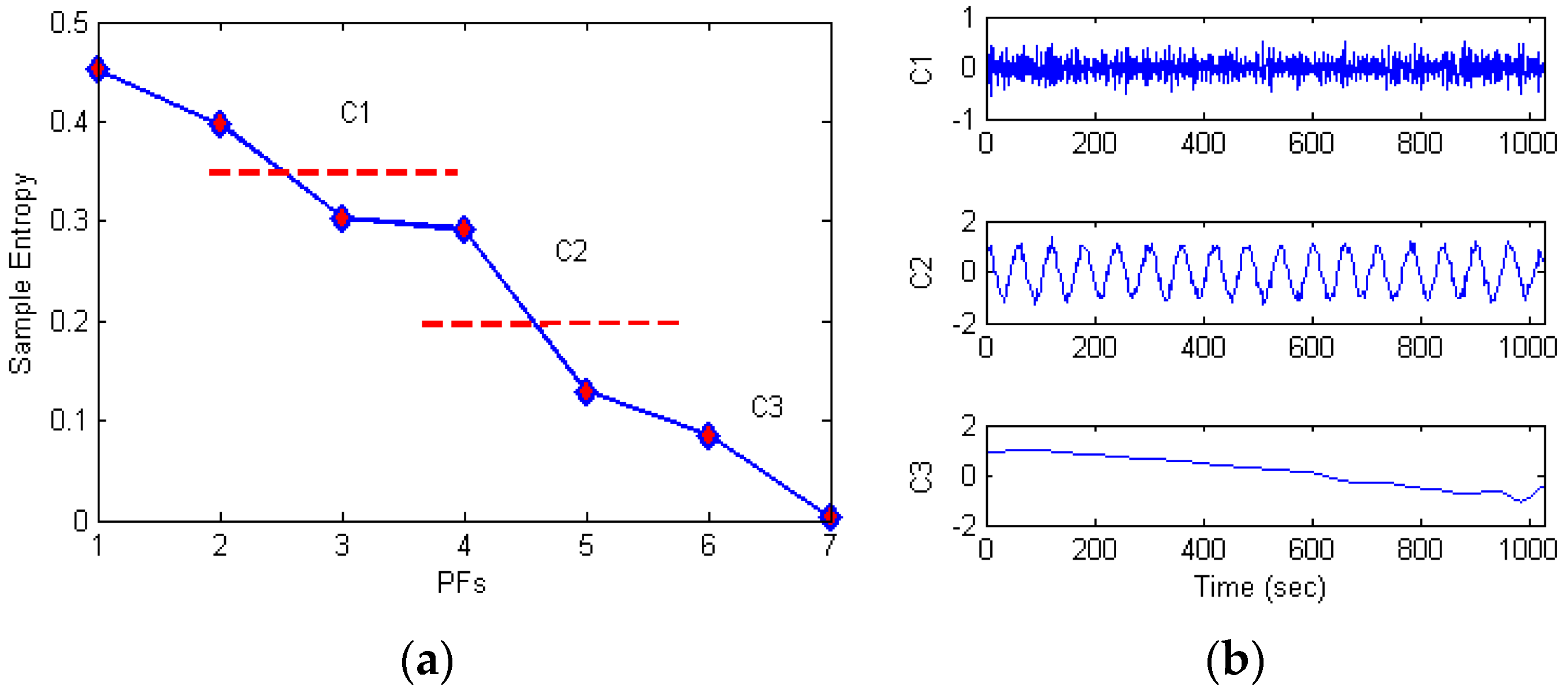
For example, there are seven PFs obtained in Figure 1. Then the SE values of each PF are calculated to classify the seven PFs into the useful component, the mixed component, and the noise component. Figure 2 shows the calculation and classification results.

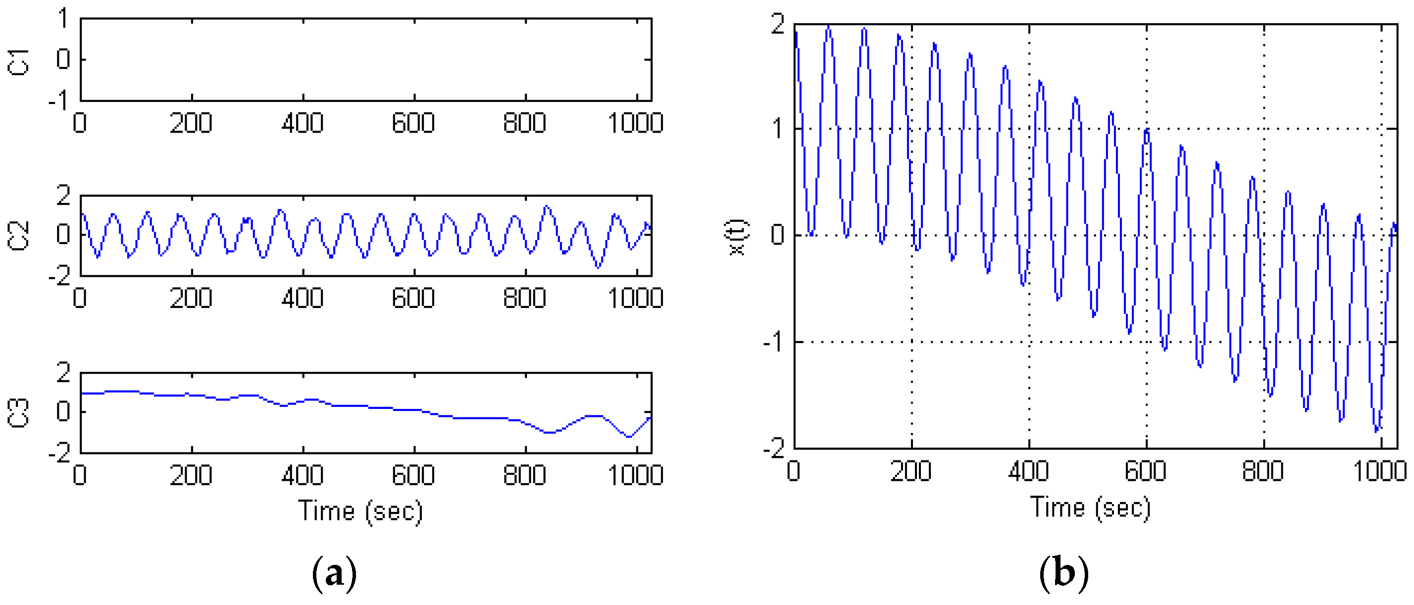
● Step 3: De-noising.

From Step 2 we can see that the useful component is consisted by low frequency PFs, the mixed component consists of useful signal and noise. It is necessary to choose different de-noising methods for the two different components. Therefore, considering the feature of TFPF, short-window TFPF is selected to process useful component (C3) in order to preserve the valid signal as much as possible, and long-window TFPF is selected to process the mixed component (C2) in order to reduce the random noise as much as possible. The noise component (C1) would be removed directly. Figure 3a shows the de-noising results of each component.

● Step 4: Reconstruction.

After de-noising, the useful component and mixed component are reconstructed, and the final signals are obtained, which is shown Figure 3b.

Figure 4 is all the steps of proposed SE-LMD-TFPF algorithm.

3. Experiments and Results

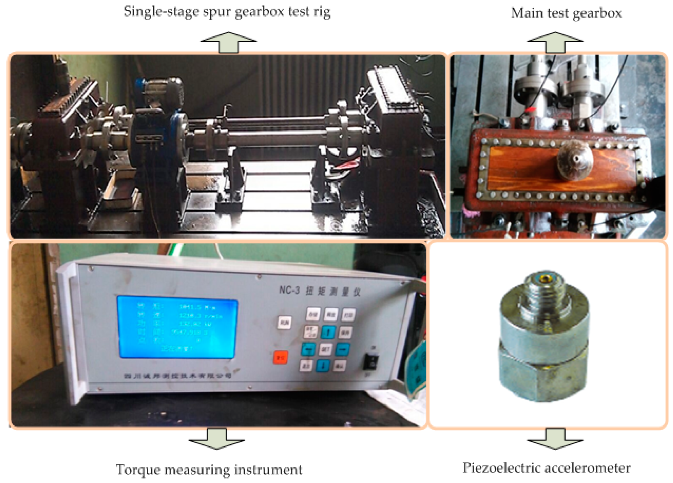
Figure 5 shows the experimental setup for signal acquisition of the gear transmission system. As shown in the figure, the experimental setup mainly consists of a main test gearbox, accompanying test gearbox, accumulator, and torsion bar. The four accumulators are installed on the bearing basis of the driving gear and driven gear. The parameters of the single-stage spur gearbox are as follows: the numbers of driving gear teeth and driven gear are 30 and 45, respectively, the module is 4 mm, the pressure angle 20°, tooth width is 40 mm, and gears are made from 45 steel. The gear ratio of the gearbox is 1:1.5. The torque is set as 408 Nm, the rotation rate is 327 r/min, and the effective power is 13.9 kW. The type of torque measuring instrument is a NC-3 (Chengbang Science and Technology, Chengdu, China). The sampling frequency is 600 Hz. The accelerometer is set on the test-bed, which is comprised of a piezoelectric accelerometer, of the type CA-YD-186 (Sinocera Piezotronics Inc., Yangzhou, China). The axial sensitivity of the CA-YD-186 is 100 mV/g, the frequency range is 0.5–6 kHz and the range of measurement is 50 g.

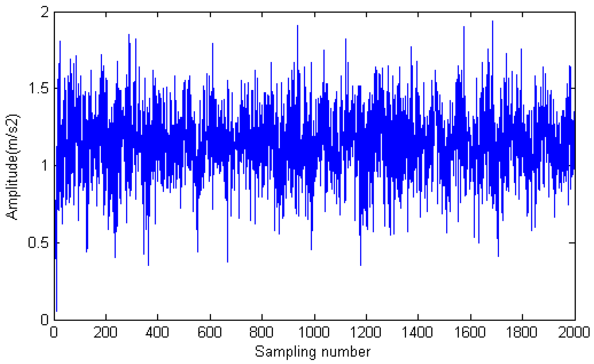
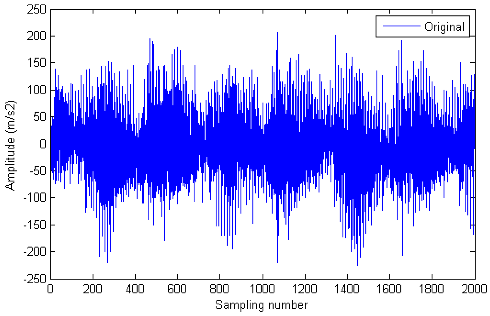
Figure 6 is the output of vibration signal from gearbox. From Figure 6 we can see that the valid signal is submerged in the noise. Therefore, it is necessary to reduce the noise.

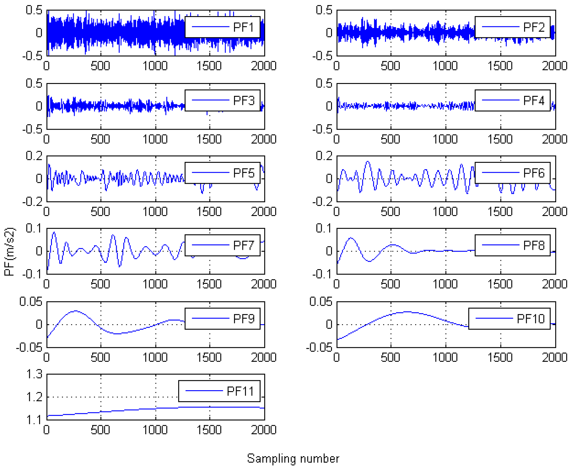
Figure 7 shows the PFs decomposed by LMD, and 11 PFs are obtained. According to the hybrid de-noising algorithm proposed by [16], each PF would be filtered. Obviously, the computation cost would be increased greatly. In our study, sample entropy is introduced to calculate the similarity of PFs, and the PFs with strong similarity would be classified into one component.

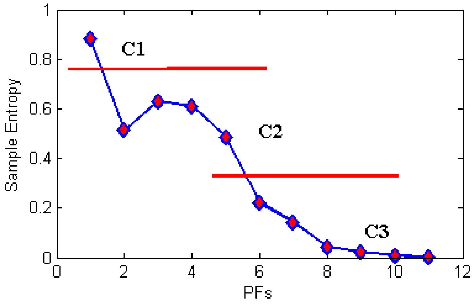
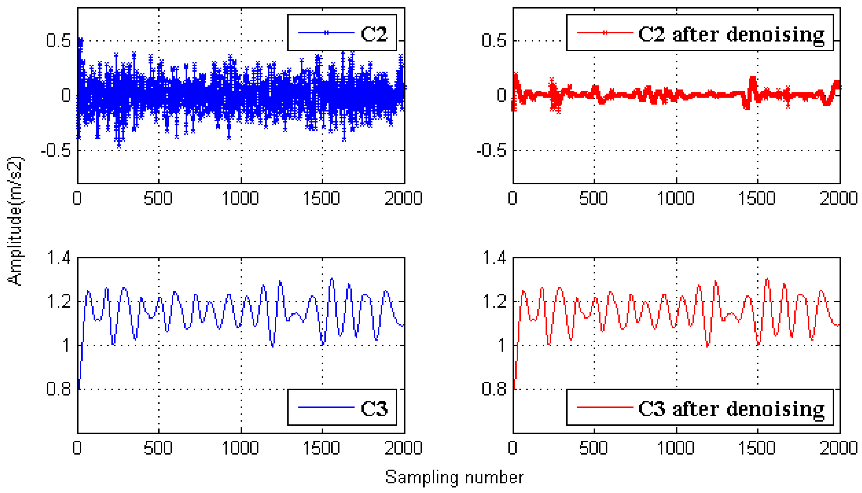
As shown in Figure 8, PF1 is classified as a noise component (C1), PF2 to PF5 are classified as the mixed component (C2) and PF6 to PF11 are classified as the useful component (C3).

Figure 9 shows the de-noising results of C2 and C3. The original C2 has significant noise; therefore, the long-window TFPF is employed, and we can see that the random noises are suppressed effectively. The original C3 is the component with valid signals; therefore, the short-window TFPF is employed, and we can see that the valid signal amplitude is preserved effectively.

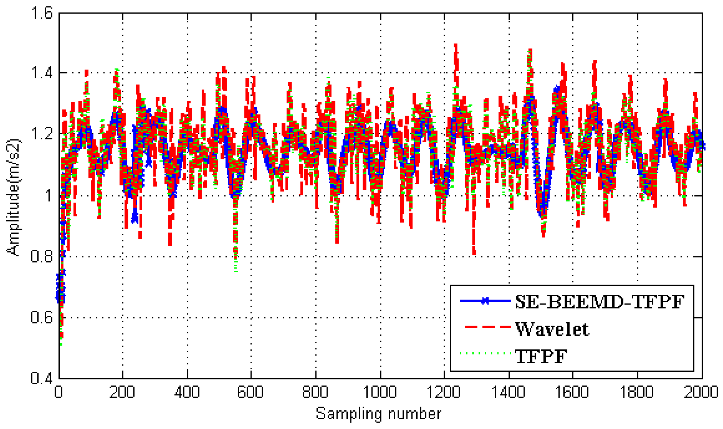
Wavelet de-noising and traditional TFPF algorithms (where the window length is fixed) are employed to filter the original gear signal for comparison. Symlet function is an approximate symmetrical wavelet function proposed by Daubechies, which is an improvement of db functions. Therefore, in the wavelet de-noising process, sym5 is selected as the wavelet basis and the the decomposition level is selected as 3, by experience; the fixed wavelength of the TFPF is also selected by experience. Figure 10 is the comparison results. From Figure 10 we can see that after wavelet de-noising, the randomness of the signal still exists and it is obvious that the de-noising result of TFPF is better than the wavelet method and the proposed SE-LMD-TFPF can restrain the randomness of the signal effectively. Therefore, it can be concluded that compared to the wavelet method and TFPF algorithm, the proposed SE-LMD-TFPF algorithm has the best de-noising result. The random noises are reduced effectively and the valid signals are preserved.

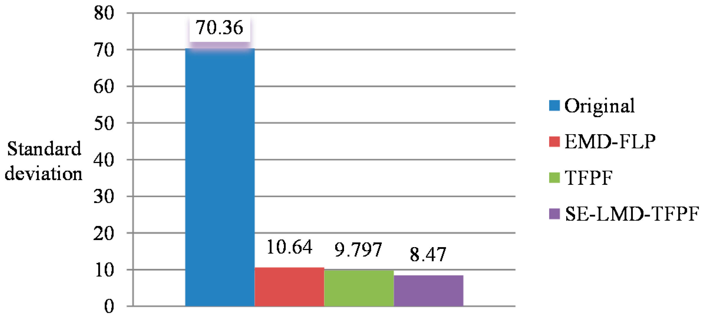
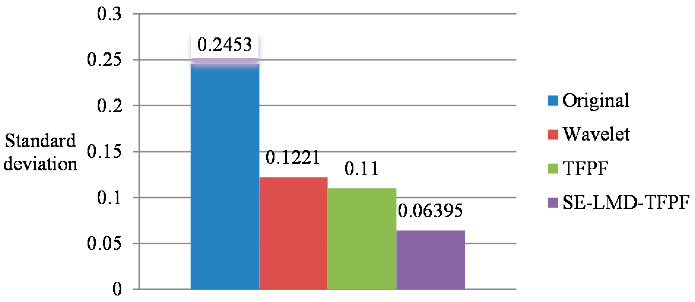
Moreover, standard deviation is employed to evaluate the de-noising results. Figure 11 shows the comparison results which prove that the proposed SE-LMD-TFPF has the best de-noising results with the lowest standard deviation.

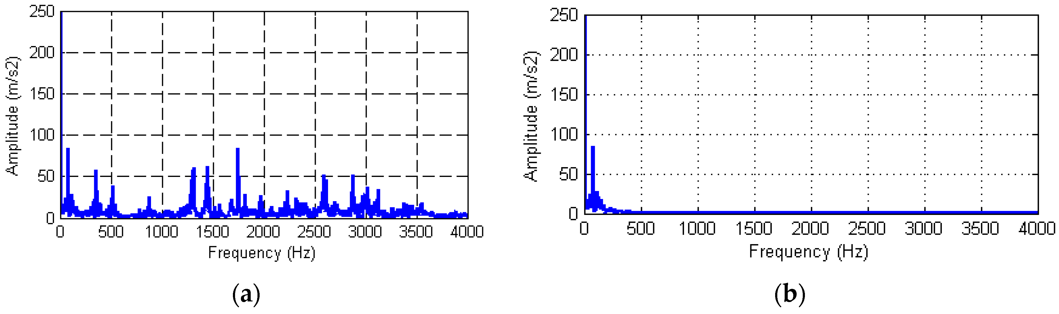
Figure 12 shows the FFT of the original signal and the signal denoised by SE-LMD-TFPF. From Figure 12, it can be clearly seen that most of the high frequency content of the signal have been removed, and the lowest frequency components have been effectively kept. Therefore, it can be concluded that the de-noising performance of the proposed SE-LMD-TFPF algorithm is favorable.

In order to verify the effectiveness of the proposed SE-LMD-TFPF de-noising algorithm, another set of experiments is carried out and the data are employed for verification. In the experiment, the torque is set as 193 Nm, the rotation rate is 1200 r/min, and the power is 24.8 kW. Figure 13 is the output of vibration signal from gearbox and the sampling frequency is 8000 Hz. 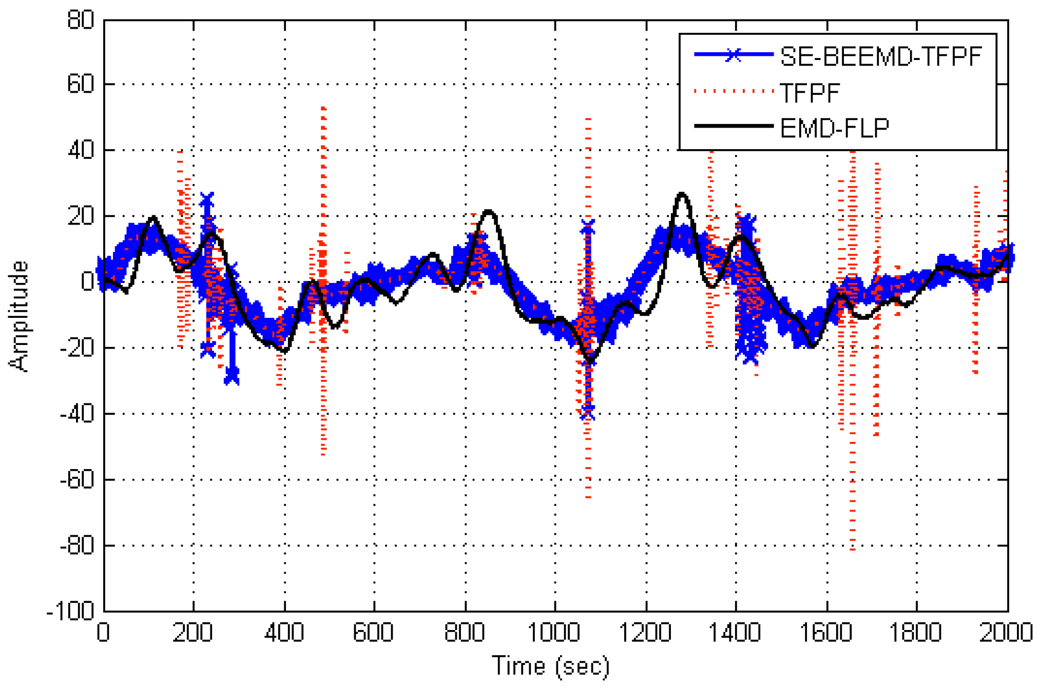Similar to Figure 6, the valid signal is also submerged in the noise in Figure 13. The de-noising process is the same as previously shown, containing decomposition, classification, de-noising, and reconstruction. Finally, the reconstructed signals are obtained, as shown in Figure 14.

In Figure 14, the EMD-FLP denoising algorithm [24] is introduced for comparison. It can be clearly seen that, compared to EMD-FLP and TFPF algorithms, the proposed SE-LMD-TFPF algorithm has the best de-noising result, the random noises are reduced and the valid signals are effectively preserved. Figure 15 is the comparison of standard deviations, which also prove that the proposed SE-LMD-TFPF algorithm has the best de-noising ability.

Table 1. Comparison between TFPF and SE-LMD-TFPF.

	Standard Deviation (m/s2)	Computation Time (s)
TFPF	9.797	0.76
SE-LMD-TFPF	8.474	2.85

shows the detailed de-noising performance and computation time comparison between TFPF and SE-LMD-TFPF algorithms by using the data of Figure 10. Obviously the de-noising performance of SE-LMD-TFPF is better than TFPF algorithm, but it also can be found that the time cost by TFPF is just 0.76 s and the SE-LMD-TFPF is 2.85 s. Therefore, it can be concluded that, compared to the traditional TFPF method, the proposed SE-LMD-TFPF is more suitable for offline signal processing.

4. Conclusions

In this paper, a novel de-noising algorithm based on LMD, SampEn, and TFPF is proposed for reducing the random noise of a gear transmission system. It is an improvement of the conventional TFPF method, which applies the decomposition characteristics of LMD and SampEn to bring flexibility to TFPF in selecting the window length. Experiments on gearbox data demonstrate that the proposed method makes a good tradeoff in random noise reduction and valid signal preservation, especially compared with traditional TFPF method.

Additionally, the proposed SE-LMD-TFPF de-noising algorithm is only applied to a signal with a low signal-to-noise ratio without obvious shock and vibration, the purpose of this paper being to verify the de-noising performance of the proposed method.Obviously, the effectiveness of the SE-LMD-TFPF algorithm is verified by the calculation results of standard deviations. In our next work, the SE-LMD-TFPF algorithm will be applied to signals with obvious shock or vibration and fault diagnosis.