Article

Efficient Multi-Label Feature Selection Using Entropy-Based Label Selection

School of Computer Science and Engineering, Chung-Ang University, 221 Heukseok-Dong, Dongjak-Gu, Seoul 156-756, Korea
*
Author to whom correspondence should be addressed.
Entropy 2016, 18(11), 405; https://doi.org/10.3390/e18110405
Submission received: 15 July 2016 / Revised: 4 October 2016 / Accepted: 10 November 2016 / Published: 15 November 2016

Abstract

:
Multi-label feature selection is designed to select a subset of features according to their importance to multiple labels. This task can be achieved by ranking the dependencies of features and selecting the features with the highest rankings. In a multi-label feature selection problem, the algorithm may be faced with a dataset containing a large number of labels. Because the computational cost of multi-label feature selection increases according to the number of labels, the algorithm may suffer from a degradation in performance when processing very large datasets. In this study, we propose an efficient multi-label feature selection method based on an information-theoretic label selection strategy. By identifying a subset of labels that significantly influence the importance of features, the proposed method efficiently outputs a feature subset. Experimental results demonstrate that the proposed method can identify a feature subset much faster than conventional multi-label feature selection methods for large multi-label datasets.

1. Introduction

Multi-label learning is the process of identifying useful relations between target labels and input data. Examples include taxonomies of email corpuses from texts or the emotive qualities of music from audio sources [1,2,3,4]. This technique is useful for learning a model when input patterns can be associated with multiple labels concurrently [5,6,7,8,9,10]. For example, in practice, applications can employ a series of labels to encode target concepts to be learned, especially when the target consists of multiple sub-concepts, such as humor or admiration [11,12]. Let W R d denote a set of training patterns constructed from a set of features F. Then, each pattern w i W where 1 i | W | is assigned to a certain label subset λ i L , where L = { l 1 , , l | L | } and is a finite set of labels. In order to represent the label association of training pattern-label set pair ( w i , λ i ) , each label can be encoded using a binary vector b = ( b 1 , , b | L | ) = { 0 , 1 } | L | representing the joint state of the label set where each element is one if the label is relevant and zero otherwise [13]. Under the multi-label learning umbrella, the goal of multi-label feature selection is to determine a subset of important features for multiple labels [14,15,16]. This problem can be solved by selecting a subset S composed of n features from F that jointly have the largest dependency on the labels L. Thus, multi-label feature selection can be achieved through a scoring process that assesses the importance of | F | features and selects the top-ranked n | F | features for inclusion in the feature subset S [17]. This technique is particularly useful for reducing the cost of collecting features, understanding the underlying mechanism connecting input features and multiple labels, possibly improving the predictive performance and shortening the learning time [15,18,19]. In particular, because it can reduce the computational cost of subsequent learning methods by reducing the dimensionality of the input data, it is regarded as a promising technique for applications that involve strict time constraints [20,21,22,23,24]. In this study, we focus on accelerating the multi-label feature selection process itself, as well as the later employed learning method, such as a multi-label classifier.
Several researchers have dedicated efforts to selecting important features for multi-label learning [25,26,27,28,29]. Multi-label feature selection methods can be categorized into three types, according to how they assess the importance of candidate feature subsets [17,19]. Namely, these are the wrapper, embedded and filter approaches. Wrapper-based multi-label feature selection methods assess the importance of feature subsets based on the accuracy of a multi-label learning algorithm [30,31]. Some multi-label learning algorithms have a feature selection process embedded in their learning process [27,32]. In contrast, filter-based multi-label feature selection methods determine a feature subset by focusing on the characteristics of candidate feature subsets and multiple labels [18,28,33,34]. In this study, we construct our proposed method based on the filter approach, on account of its efficient process for identifying the final feature subset without requiring an interaction with an additional learning method [14,35].
In applications with strict time constraints, the computational efficiency of a multi-label feature selection method is clearly an important issue. However, a high efficiency may not be achieved when the method faces a large label set, because the computational cost for scoring the importance of features increases according to the number of labels [14,17,18]. Thus, when the task involves a large number of labels, the scoring process against L should be economized, to achieve an efficient multi-label feature selection. In this paper, we propose an efficient multi-label feature selection method that can quickly output a feature subset based on a new entropy-based label selection strategy. The proposed method reduces the computational cost of evaluating the feature importance by separating the process into two parts: an exact calculation quantifying the dependency (i.e., importance) between the feature and each label in the promising label set and an approximation of the dependency between the feature and influential labels. Figure 1 presents a schematic of the proposed method with our label selection strategy. For given a feature f 1 and six labels { l 1 , , l 6 } (left), the proposed method first identifies a subset of promising labels { l 1 , l 2 , l 3 } that would significantly influence the importance of the feature f 1 (middle). Finally, as shown in the right figure, the proposed method determines the importance of f 1 by calculating the dependency between f 1 and promising labels precisely, while approximating the dependency between f 1 and the remaining labels.
To the best of our knowledge, this is the first study to accelerate the multi-label feature selection method through an explicit label subset selection strategy. Our theoretical analysis and empirical experiments show that the computational cost can be reduced according to the size of the promising label set, without incurring significant changes in the multi-label learning performance.

2. A Brief Review of Multi-Label Feature Selection

A major trend in multi-label feature selection studies involves applying a feature selection method after transforming label sets into one or more labels [16,25,36]. Based on this approach, the feature selection process can be performed after the transformation process is completed. One well-known problem of the transformation method in this approach is Binary Relevance (BR), which separates each label independently [34]. After separating the label set, a score function that is able to measure the importance of features and labels, such as the Pearson correlation coefficient (BR + CC) [37] or odds ratio (BR + OR) [38], can be employed. Because the final feature score is obtained by aggregating all of the importance values of (feature, label) pairs, it requires a prohibitive computational cost if a large label set is involved. On the other hand, efficient multi-label feature selection may not be achieved if the transformation process consumes excessive computational resources. For example, ELA + CHI evaluates the importance of each feature using χ 2 statistics (CHI) between the feature and a single label obtained by using Entropy-based Label Assignment (ELA), which separates multiple labels and assigns them to duplicated patterns [25]. Thus, the label transformation process will require a prohibitive execution time if the multi-label dataset is composed of a large number of patterns and labels. Although the computational cost of the transformation process can be remedied by applying a simple procedure [16,39], an inefficient feature selection process can occur if the scoring process incurs excessive computational costs when evaluating the importance of features [26,34]. For example, PPT + RF identifies appropriate weight values for features based on a label that is transformed by the Pruned Problem Transformation (PPT) [39] and the conventional ReliefF (RF) scheme for single-label feature selection [40]. Although the ReliefF method can be extended to handle multi-label problems directly [35], the execution time to obtain the final feature subset can be excessively high if the dataset is composed of a large number of patterns, because ReliefF requires similarity calculations for pattern pairs.
In addition to the merits and side effects resulting from the immediate use of conventional methods [41], algorithm adaptation strategies attempt to handle the problem of multi-label feature selection directly [15,17,18,27,29,33]. In this approach, a feature subset is obtained by optimizing a specific criterion (the name of corresponding multi-label feature selection method is presented in the parenthesis if it is suggested by authors); a joint learning criterion involving feature selection and multi-label learning concurrently [32,42], l 2 , 1 -norm function optimization (RFS) [29], a Hilbert–Schmidt independence criterion (gMLC) [33], label ranking errors [27], F-statistics (MFS) [28], label-specific feature selection (LIFT) [9] or memetic feature selection based on mutual information (MAMFS) [30]. However, if multi-label feature selection methods based on this strategy consider all features and labels at once, the scoring process can be computationally prohibitive or even fail, owing to the internal task of finding an appropriate hyperspace using pairwise pattern comparisons [27], a dependency matrix calculation [33] and iterative matrix inverse operations [29]. As a promising starting point for reducing the computational cost, the work of [18] demonstrated that mutual information can be decomposed into a sum of dependencies among variable subsets (PMU), which is a very useful property for solving multi-label learning problems [9,17]. In a similar approach, the dependency calculation for feature and label pairs has been discarded (D2F) [14], and feature dependency has been normalized using the number of previously-selected features (MDMR) [15]. More efficient score functions, specialized into an incremental search strategy and a quadratic programming framework, have also been considered, in methods known as AMI [43] and QPMLFS [44], respectively. However, these mutual information-based score functions commonly require the calculation of the dependencies between all variable pairs composed of a feature and a label. Thus, they share the same drawback in terms of computational efficiency, because labels known to have no influence on the evaluation of feature importance are included in the calculations as FIMF [17].
Although the characteristics of multi-label feature selection methods can vary according to how the importance of features is modeled, conventional methods create a feature subset by scoring the importance of features either for all labels [16,25,33] or all possible combinations drawn from the label set [17,18,27]. Thus, these methods inherently suffer from prohibitive computational costs when the dataset is composed of a large number of labels. In this study, we will demonstrate that the computational cost of evaluating the importance of features against a set of influential labels can be reduced using our new label selection strategy, resulting in the acceleration of the feature selection process. The contribution of this study can be summarized as follows:
  • To accelerate multi-label feature selection processes involving large numbers of labels, we propose a novel entropy-based label selection strategy to identify promising labels.
  • To prevent the degradation of feature identification capability, a theoretical analysis is performed regarding the process of evaluating feature importance in the multi-label situation.
  • To preserve the computational cost, the proposed label selection method is designed to rely on calculations that can be reused in the later feature selection process.
  • In previous studies [14,17,18], the multi-label feature selection methods consider all of the labels to identify an important feature subset. In contrast, we present a novel method that is able to identify the important feature subset based on a subset of labels.

3. Proposed Method

3.1. Characteristics of Feature Importance and a Strategy to Reduce the Computational Cost

In this study, we focus on a mutual information-based multi-label feature selection method, owing to the existence of thorough discussions regarding its theoretical background [14,17,18,43] and its popularity [15,26,30,44,45]. Given a feature set F and label set L, the dependency, or shared entropy, between F and L can be measured using mutual information as follows [46]:
M ( F ; L ) = H ( F ) H ( F , L ) + H ( L )
where H ( X ) = x X P ( x ) log P ( x ) is the joint entropy with probability function P ( x ) . If x is a joint state of variables in X, then the entropy can be calculated directly. On the other hand, if the given variable set X contains a set of numerical variables, then the entropy of X can be obtained by discretizing each variable in X [47] or using the concept of differential entropy [48]. In practice, direct computation of Equation (1) can be impractical, because an inaccurate probability estimation can occur on account of the high dimensionality of a large label set L or an insufficient number of patterns [14]. To circumvent this difficulty, Equation (1) can be rewritten as [18]:
M ( F ; L ) = k = 2 | F | + | L | m = 1 k 1 ( 1 ) k V k ( F k m × L m )
where × is the Cartesian product between two sets and V k ( · ) is the sum of a k-degree interaction, defined as [14]:
V k ( X ) = Y X k I ( Y )
where X is a power set of X without { } , Y is a possible element from X k = { e | e X , e = k } and I ( Y ) is the interaction information involving a variable set Y. Specifically, this is defined as [49]:
I ( Y ) = Z Y ( 1 ) Z H ( Z )
For example, if F = { f 1 } and L = { l 1 , l 2 } , then M ( F ; L ) can be rewritten as:
M ( F ; L ) = V 2 ( F 1 × L 1 ) V 3 ( F 1 × L 2 ) = i = 1 | F | j = 1 | L | I ( f i , l j ) i = 1 | F | j = 1 | L | k = j + 1 | L | I ( f i , l j , l k )
Equation (2) indicates that the interaction information for all possible variable subsets across F and L influences the dependency between F and L. Thus, it also indicates that the computational cost of calculating Equation (2) increases exponentially according to the number of labels. To circumvent intractable computational costs, Equation (2) can be approximated by setting a parameter that adjusts the maximum allowed cardinality of variable subsets [14,17]:
M ˜ b ( F ; L ) = k = 2 b m = 1 k 1 ( 1 ) k V k ( F k m × L m )
where 2 b | F | + | L | . Equation (5) indicates that the computational cost can be significantly reduced by setting b = 2 , as follows:
M ˜ 2 ( F ; L ) = k = 2 2 m = 1 k 1 ( 1 ) k V k ( F k m × L m ) = m = 1 1 ( 1 ) 2 V 2 ( F 2 m × L m ) = V 2 ( F 1 × L 1 )
Equation (6) indicates that the dependency between F and L can be approximated by summing over all of the interaction information terms of variable subsets containing a feature and a label. Thus, a function D ( F , L ) that measures the dependency between F and L can be written as:
D ( F , L ) = V 2 ( F 1 × L 1 ) = f F l L I ( f , l )
For simplicity, the interaction information term for a variable subset involving only two variables can be rewritten using the mutual information terms relating to the variable subset, as follows:
I ( x , y ) = Z { x , y } ( 1 ) | Z | H ( Z ) = H ( x ) + H ( y ) H ( x , y ) = M ( x ; y )
As a result, D ( F , L ) can be rewritten as:
D ( F , L ) = f F l L M ( f ; l )
Equation (8) indicates that all mutual information terms for all possible pairs ( f , l ) with f F and l L should be calculated to perform a multi-label feature selection based on D ( F , L ) . Because each feature in F contributes to D ( F , L ) independently, the optimal feature subset can be obtained by selecting the top n features with the largest contributions (i.e., importance) to the value of D ( F , L ) . This is calculated as:
C ( f ) = l L M ( f ; l ) = | L | · H ( f ) l L H ( f , l ) + l L H ( l )
where f F . Equation (9) indicates that when the label set L is large, the scoring process may incur high computational costs, because it must calculate the joint entropy term H ( f , l ) . To reduce the computational cost, C ( f ) should be approximated. Shannon’s inequality for information entropy indicates that M ( f ; l ) is bounded as [46]:
0 M ( f ; l ) K ( f , l )
where K ( a , b ) = min H ( a ) , H ( b ) . Because the term K ( f , l ) does not involve the calculation of the joint entropy term H ( f , l ) , the scoring process can be accelerated by approximating the M ( f ; l ) term using the K ( f , l ) term. As a result, C ( f ) can be approximated as:
C ˜ ( f ) = l L K ( f , l ) = l L min H ( f ) , H ( l )
In this study, Equation (11) will be used to calculate the dependency between features and influential labels, in order to reduce computational costs. Suppose that a multi-label feature selection method employs Equation (11) to evaluate the feature importance, where the joint dependency between features and labels is not considered. Then, the importance of features is determined by the features’ own entropy values.
Proposition 1.
If H ( a ) H ( b ) , then C ˜ ( a ) C ˜ ( b ) .
Proof. 
Suppose that there are two features a , b F , where H ( a ) H ( b ) . Because the importance of a and the importance of b are calculated using C ˜ ( a ) and C ˜ ( b ) , the inequality C ˜ ( a ) C ˜ ( b ) will hold if each K ( a , l ) value is greater than or equal to the corresponding K ( b , l ) value with the same label l. When H ( a ) H ( b ) , the value of K ( a , l ) is always greater than or equal to the corresponding K ( b , l ) value, because the following relations are satisfied:
  • If H ( a ) H ( b ) H ( l ) , then K ( a , l ) = K ( b , l ) = H ( l ) .
  • If H ( a ) H ( l ) H ( b ) , then K ( a , l ) = H ( l ) and K ( b , l ) = H ( y ) , and thus, K ( a , l ) K ( b , l ) .
  • If H ( l ) H ( a ) H ( b ) , then K ( a , l ) = H ( a ) and K ( b , l ) = H ( b ) , and thus, K ( a , l ) K ( b , l ) .
Because these relations hold for all pairs K ( · , · ) , a will correspond to a value C ˜ ( a ) that is greater than or equal to the value of C ˜ ( b ) . ☐
Proposition 1 indicates that the computational cost can be significantly reduced, because the scoring process can be performed without calculating the terms H ( f , l ) . On the other hand, it also indicates that features with higher entropy values will be included in the final feature subset S, regardless of their dependencies with labels. Because the feature subset should depend on L, a strategy to enhance the dependency between S and L without incurring an excessive computational cost is required. To establish a proper strategy, the characteristics of C ˜ ( f ) against C ( f ) should be investigated. First, we state Proposition 2 as follows.
Proposition 2.
C ˜ ( f ) is the upper bound of C ( f ) , written as:
0 C ( f ) C ˜ ( f )
Proof. 
Equation (9) shows that C ( f ) is the sum of the mutual information terms between f and all labels. Because each M ( f ; l ) term is bounded above by each K ( f , l ) term with the same label l and C ˜ ( f ) is the sum of all the K ( f , l ) terms, C ˜ ( f ) is always greater than or equal to C ( f ) . ☐
Proposition 2 indicates that a multi-label feature selection method employing C ˜ ( f ) for the scoring process, such as multi-label feature selection based on D ( F , L ) , may imply the identification of a feature subset that is far away from a designated solution if the value of C ˜ ( f ) is dissimilar to C ( f ) . Thus, a strategy for fine-tuning the C ˜ ( f ) function towards the C ( f ) function, within the constraints of given computational resources, would be beneficial. In a multi-label feature selection method based on D ( F , L ) , the method may repeatedly calculate the mutual information terms, along with l L , in order to obtain the value of C ( f ) . Within this loop, let us define a function C ˜ j ( f ) , where j is the number of labels considered for calculating the mutual information terms, as follows:
Definition 1.
Let Y L be the labels for which the actual mutual information between given features f and l Y is calculated, where | Y | = j . Then, the score function C ˜ j ( f ) is defined as:
C ˜ j ( f ) = l Y M ( f ; l ) + l Y c K ( f , l )
where Y is a set of labels already considered during the loop, | Y | = j , Y c is a complementary set of Y and Y Y c = L . Thus, C ˜ 0 ( f ) = C ˜ ( f ) and C ˜ | L | ( f ) = C ( f ) . The number of calculated mutual information terms will be incremented by one during each loop iteration, leading to a series of intermediate bounds, as described in Lemma 1.
Lemma 1.
Let Y j L be the label subset Y for calculating C ˜ j ( f ) . Then, a series of bounds C j ( f ) can be identified as:
C ( f ) C ˜ | L | 1 ( f ) C ˜ j ( f ) C ˜ 1 ( f ) C ˜ ( f )
where Y j Y j + 1 .
Proof. 
For the inequality to hold, the following relation should be satisfied:
0 C ˜ j ( f ) C ˜ j + 1 ( f ) = l Y j M ( f ; l ) + l Y j c K ( f , l ) l Y j + 1 M ( f ; l ) l Y j + 1 c K ( f , l )
Equation (15) can be simplified as:
= l Y j c K ( f , l ) l Y j + 1 c K ( f , l ) l Y j + 1 M ( f ; l ) l Y j M ( f ; l ) = l { Y j c Y j + 1 c } Part 1 K ( f , l ) l { Y j + 1 Y j } M ( f ; l )
Because Y j + 1 = { Y j , y } , where y is a label and Y j c = { L Y j } , the label subset { Y j + 1 c Y j c } in Part 1 can be simplified as:
{ Y j c Y j + 1 c } = { { L Y j } { L { Y j , y } } } = { Y j , y } Y j = y
Thus, Equation (16) can be simplified as follows:
= l { y } K ( f , l ) l { y } M ( f ; l ) = K ( f , y ) M ( f ; y )
Equation (18) indicates that C ˜ j ( f ) C ˜ j + 1 ( f ) is always greater than or equal to zero. Because this relation holds for 0 j | L | 1 , Lemma 1 can be obtained, which represents a series of bounds. ☐
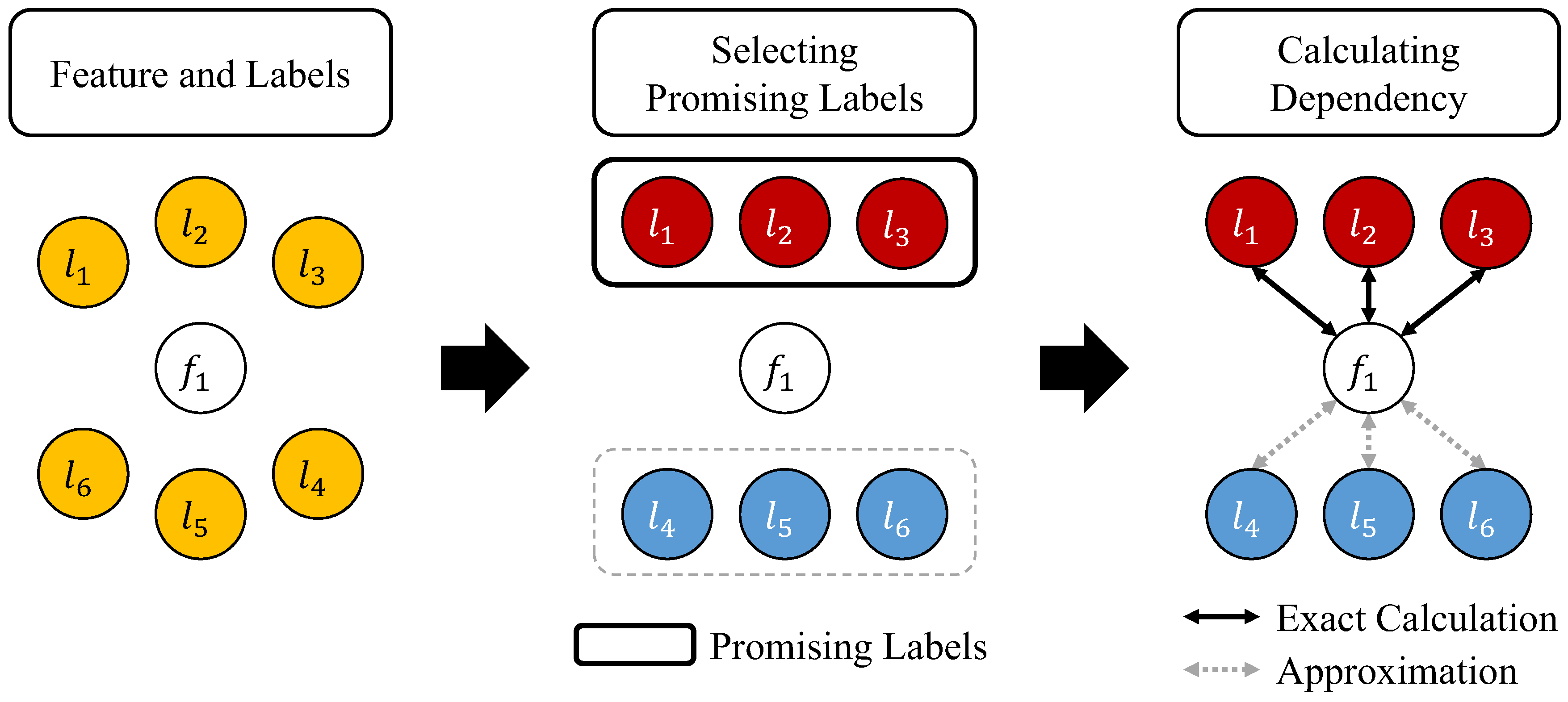
Lemma 1 indicates that it is possible to obtain a better approximation C ˜ j ( f ) for estimating C ( f ) by increasing the size of Y. That is, the ability of the function C ˜ j ( f ) to measure the importance of f in terms of the dependency between f and labels is enhanced. In other words, the algorithm is able to reduce the computational cost by selecting a proper label subset Y, because the calculation for the K ( f , l ) terms incurs a lower computational cost than that for the M ( f ; l ) terms. Suppose that the algorithm is able to identify a promising label set Y prior to the actual scoring process. Then, Lemma 1 can be generalized as Theorem 1.
Theorem 1.
Suppose that the algorithm identifies a label subset Y prior to the scoring process. By calculating the mutual information terms between f and the labels in Y, the following relation can be obtained:
C ( f ) C ˜ j ( f ) C ˜ ( f )
Proof. 
Let us begin with the lower bound of C ˜ j ( f ) . For the inequality to hold, C ˜ j ( f ) should be greater than or equal to C ( f ) . Thus, the following equation should be satisfied:
0 C ˜ j ( f ) C ( f ) = l Y M ( f ; l ) + l Y c K ( f , l ) l L M ( f ; l )
Equation (20) can be simplified as follows:
= l Y M ( f ; l ) + l Y c K ( f , l ) l Y M ( f ; l ) l Y c M ( f ; l ) = l Y c K ( f , l ) l Y c M ( f ; l ) = l Y c ( K ( f , l ) M ( f ; l ) Part 2 )
Equation (21) shows that Part 2 is always greater than or equal to zero, because each K ( f , l ) term is the upper bound of the corresponding M ( f ; l ) term with the same label l. Thus, the lower bound is always satisfied. Next, let us focus on the upper bound of C ˜ j ( f ) . To satisfy the inequality, C ˜ j ( f ) should be less than or equal to C ˜ ( f ) . Thus, the following equation should be satisfied:
0 C ˜ ( f ) C ˜ j ( f ) = l L K ( f , l ) l Y M ( f ; l ) l Y c K ( f , l )
Equation (22) can be simplified as follows:
= l Y K ( f , l ) + l Y c K ( f , l ) l Y M ( f ; l ) l Y c K ( f , l ) = l Y K ( f , l ) l Y M ( f ; l ) = l Y ( K ( f , l ) M ( f ; l ) Part 3 )
Equation (23) shows that Part 3 is always greater than or equal to zero, because each K ( f , l ) term is the upper bound of the corresponding M ( f ; l ) term with the same label l. Thus, the upper bound is also always satisfied. ☐
Theorem 1 indicates that the value of C ˜ j ( f ) is closer to C ( f ) than C ˜ ( f ) for any given label set Y, except for Y = { } . In addition, in order to obtain a value C ˜ j ( f ) similar to the value C ( f ) for efficient feature scoring with a small Y, the identification of a promising label set Y becomes an important task. Because Lemma 1 implies that C ˜ j ( f ) monotonically decreases to C ( f ) as the size of Y increases and both K ( f , a ) M ( f ; a ) and K ( f , b ) M ( f ; b ) are independent of each other where a , b Y j c , a promising label set Y that minimizes the difference between C ( f ) and C ˜ j ( f ) can be identified by including y Y c in Y sequentially in a manner that maximizes K ( f , y ) M ( f ; y ) , as shown in Equation (18). However, this task is inefficient, because it requires the calculation of all of the mutual information terms during the loop. Moreover, in this manner, the promising label set Y can be different for each feature, owing to the mutual information terms involved in Equation (18). This results in an excessive computational cost for identifying a promising label set for each feature.

3.2. An Efficient Process for Identifying a Promising Label Set

In the work of [14], it was demonstrated that the feature subset can reduce the uncertainty of labels (i.e., the remaining entropy) by using its selected features. A feature is selected because it reduces the uncertainty of labels to a greater extent than unselected features. Suppose that the algorithm identifies a label subset Y for accelerating the scoring process. Because the algorithm precisely calculates the dependency between features and labels in Y and approximates the dependency between features and labels in Y c , the feature subset will be specialized to reduce the uncertainty of labels in Y. However, there can be a subset of labels that does not significantly contribute to the uncertainty of labels, particularly in large label sets, and these labels are known to lack influence on the importance of features [17]. These observations indicate that a value C ˜ j ( f ) similar to C ( f ) can be obtained if the algorithm identifies a Y that maintains the uncertainty of L as far as possible, with a fixed number | Y | . If the uncertainty of Y is similar to that of L, then the importance of features will not change significantly compared to cases in which the importance is evaluated based on L. The uncertainty of L can be measured by using the entropy function [46]:
E ( L ) = H ( L )
Because the calculation of Equation (24) is impractical, owing to the high dimensionality of large label set L, it can be rewritten as follows [14]:
E ( L ) = k = 1 | L | ( 1 ) k V k ( L )
Equation (25) shows that the computational cost will increase exponentially according to | L | , indicating that this can incur an intractable computational cost. To circumvent prohibitive computational costs, Equation (25) can be approximated using Equation (5), by setting a parameter b:
E ˜ b ( L ) = k = 1 b ( 1 ) k V k ( L )
where 1 b | L | . Equation (26) indicates that the most efficient approximation of E ( L ) can be obtained by setting b = 1 , as follows:
E ˜ 1 ( L ) = k = 1 1 ( 1 ) k V k ( L ) = V 1 ( L ) = l L I ( l )
Because interaction information terms with only one variable can be rewritten using an entropy term involving that variable, Equation (27) can be rewritten as follows:
E ˜ 1 ( L ) = l L H ( l )
Equation (
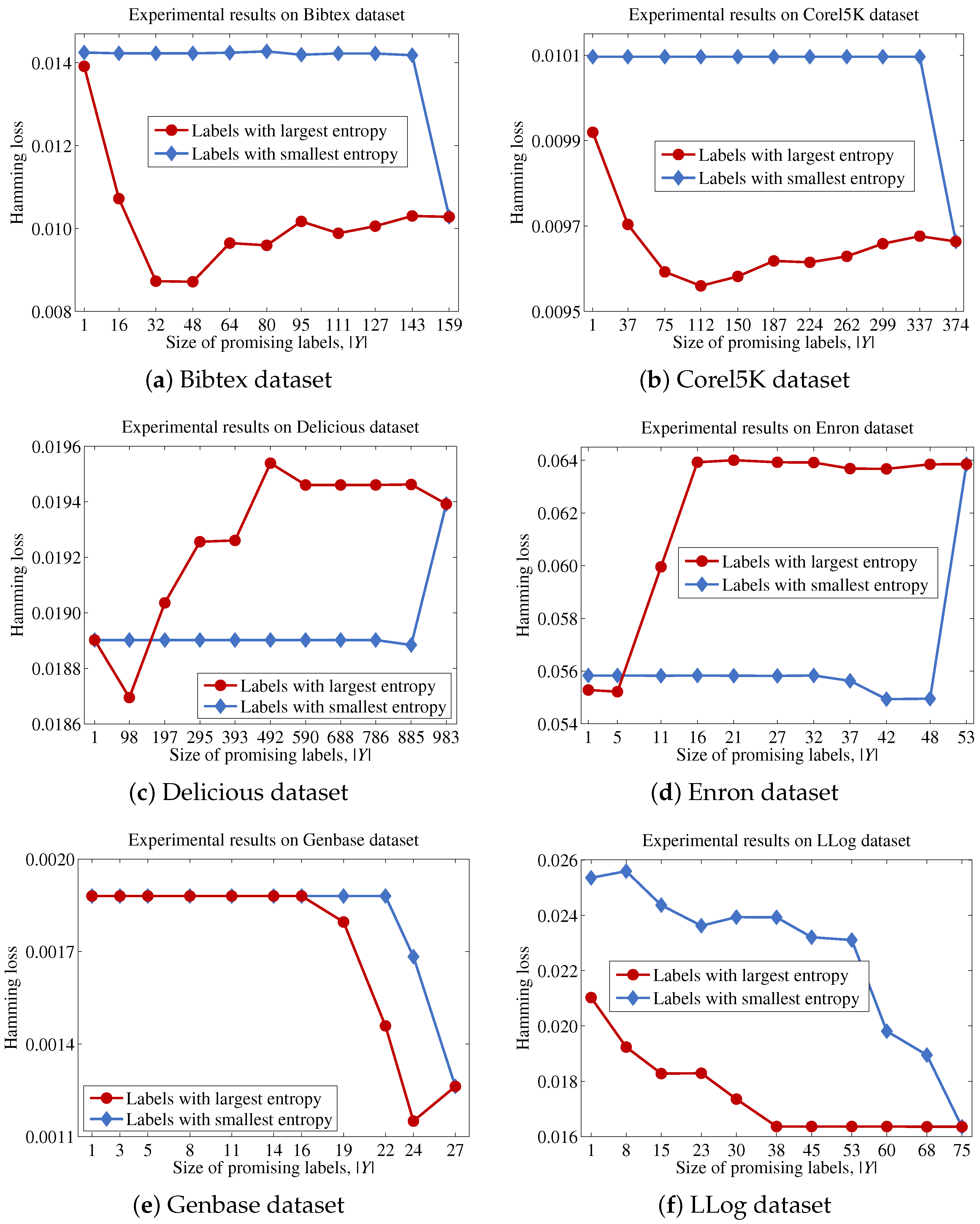
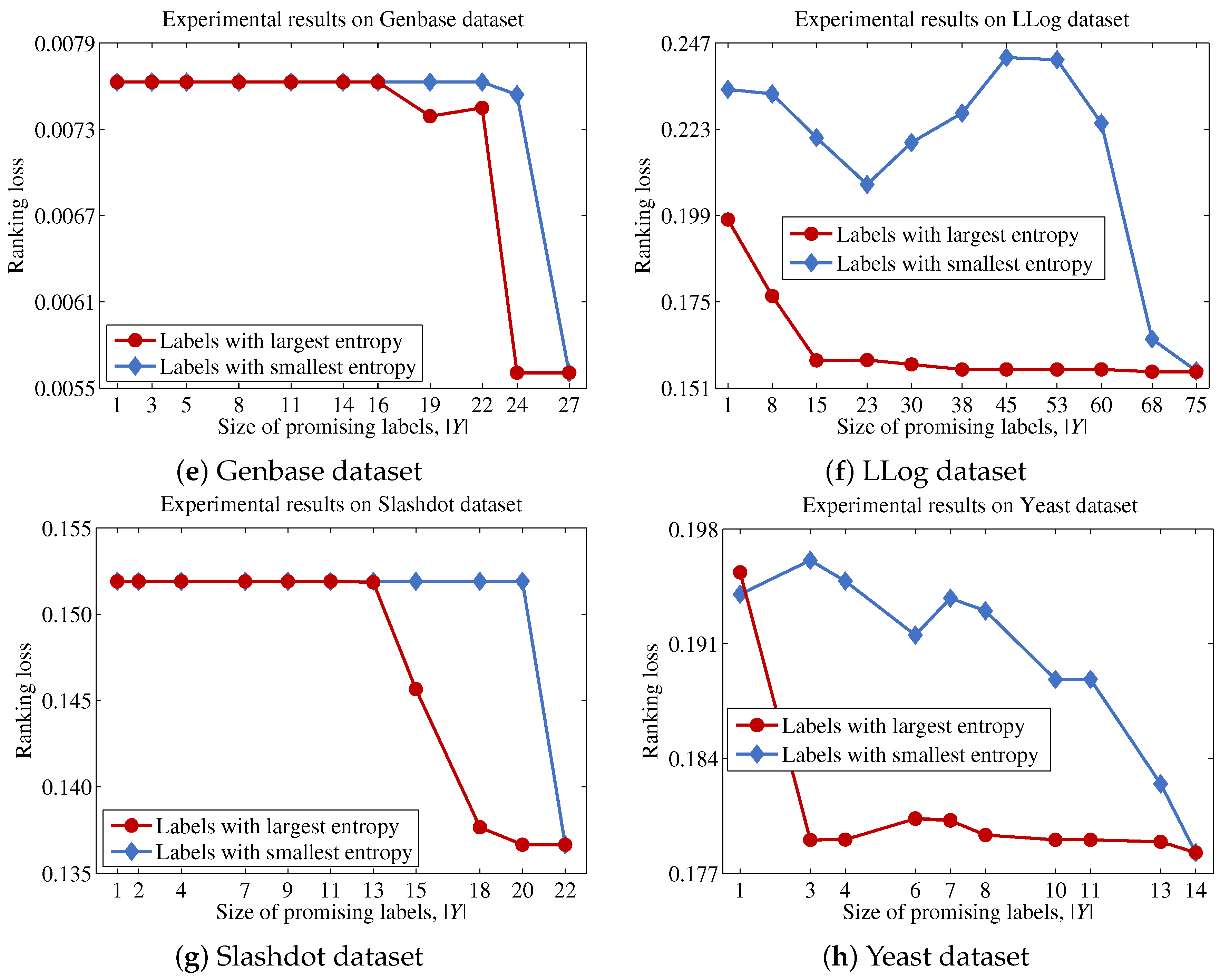
28) indicates that the uncertainty for a label set can be approximated by the sum of the entropies for each label. Because H ( · ) 0 , the optimal label set Y that maximizes E ˜ 1 ( Y ) can be obtained by selecting the top | Y | labels with the largest entropy values.
In our multi-label feature selection, C ˜ ( f ) becomes similar to C ( f ) by replacing each K ( f , l ) term with the corresponding M ( f ; l ) term that has the same label. As a result, the importance among features can be changed, because this situation occurs on all features. Let us focus on the start of the loop where Y = { } . In this step, all of the mutual information terms between f and all labels are approximated by their upper bounds, and the final score f is determined by summing over all of these values. Thus, K ( f , l ) terms where l Y c will contribute to the final score differently, because their magnitudes can vary. Based on Equation (28), the proposed method will choose a label y with the largest entropy from Y c and update the final score by replacing the K ( f , y ) term with the M ( f ; y ) term. In this case, the value of the replaced K ( f , y ) term is the largest among the values of the remaining K ( f , z ) terms on account of Theorem 2, where z { Y c y } .
Theorem 2.
The label that implies the largest K ( f , y ) value with y Y j c is the label with the largest entropy value.
Proof. 
Suppose that there are two labels a , b Y j c , with a b and H ( a ) H ( b ) . In this case, it also holds that K ( f , a ) K ( f , b ) , because H ( f ) is fixed, and the function K ( · , · ) outputs a smaller value lying between H ( f ) and the entropy value of the corresponding label. Because this relation always holds for all label pairs that can be drawn from Y j c , the inequality K ( f , a ) K ( f , b ) is always satisfied if H ( a ) H ( b ) . ☐
Because Theorem 2 is satisfied for all features, which means that the promising label at each step is the same for all features, the proposed method is able to efficiently identify the label to be considered from each step, after sorting labels based on their entropy values and choosing the label with the largest entropy from Y c sequentially. Thus, the proposed method will determine the importance of a feature by summing the mutual information values between f and labels that significantly contribute to the uncertainty of the original label set and the approximated values between f and labels with small contributions to the original label set.
Algorithm 1 describes the procedural steps of the proposed method. The proposed method first initializes F * using F (Line 6). Next, the entropy of each label in L is calculated, and then, L * is created by sorting labels based on their entropy values (Line 7). This process prevents the occurrence of repetitive sorting operations for each feature in identifying the most promising label at each step. Next, the proposed method calculates the contribution of each feature C ˜ ( f i ) (Lines 8–10). It should be noted that the recalculation of H ( l j ) to obtain M ( f i ; l j ) = H ( f i ) H ( f i , l j ) + H ( l j ) and K ( f i , l j ) = min ( H ( f i ) , H ( l j ) ) is unnecessary, because these values have been calculated in Line 7. Finally, the proposed method sorts features in F * based on the C ˜ ( · ) values for each feature and then outputs the top n features in F * (Lines 11 and 12).
Algorithm 1 Pseudo-code of the proposed method.
1:Input:
2:  F, L, n, | Y | ; where F is a set of original features, L is a set of original labels, n is the number of features to be selected and | Y | is the number of labels to be considered.
3:Output:
4:  S; where S is the final feature subset with n features.
5:Process:
6:  Create F * = { f 1 , , f | F | } by assigning F to F * ;
7:  Create L * = { l 1 , , l | L | } by sorting L using H ( l ) where l L ;
8:  for all f i F * do
9:     C ˜ ( f i ) j = 1 | Y | M ( f i ; l j ) + j = | Y | + 1 | L | K ( f i , l j ) ;
10:  end for
11:  Sort F * based on C ˜ ( · ) values;
12:  Output the top n features in F * .
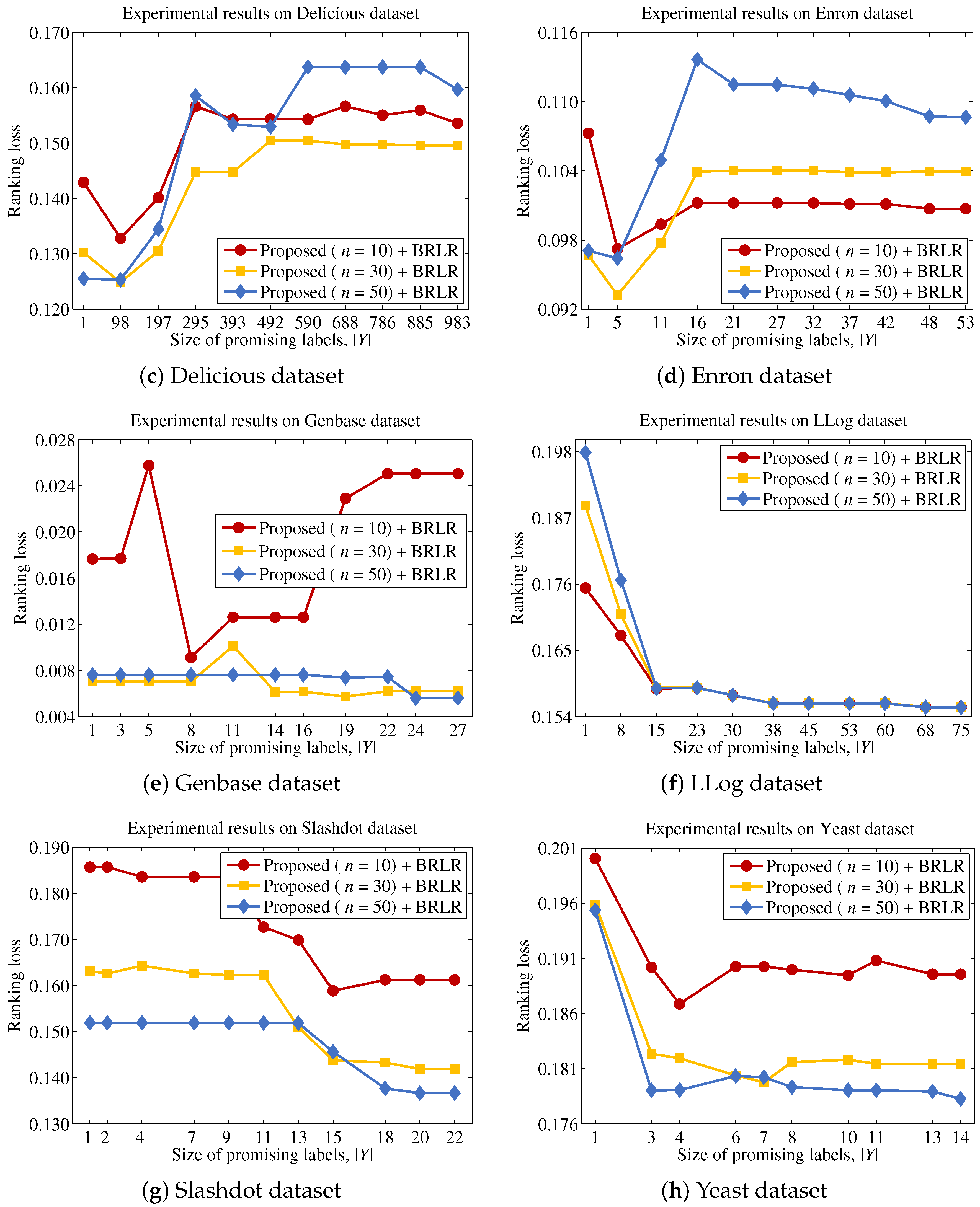
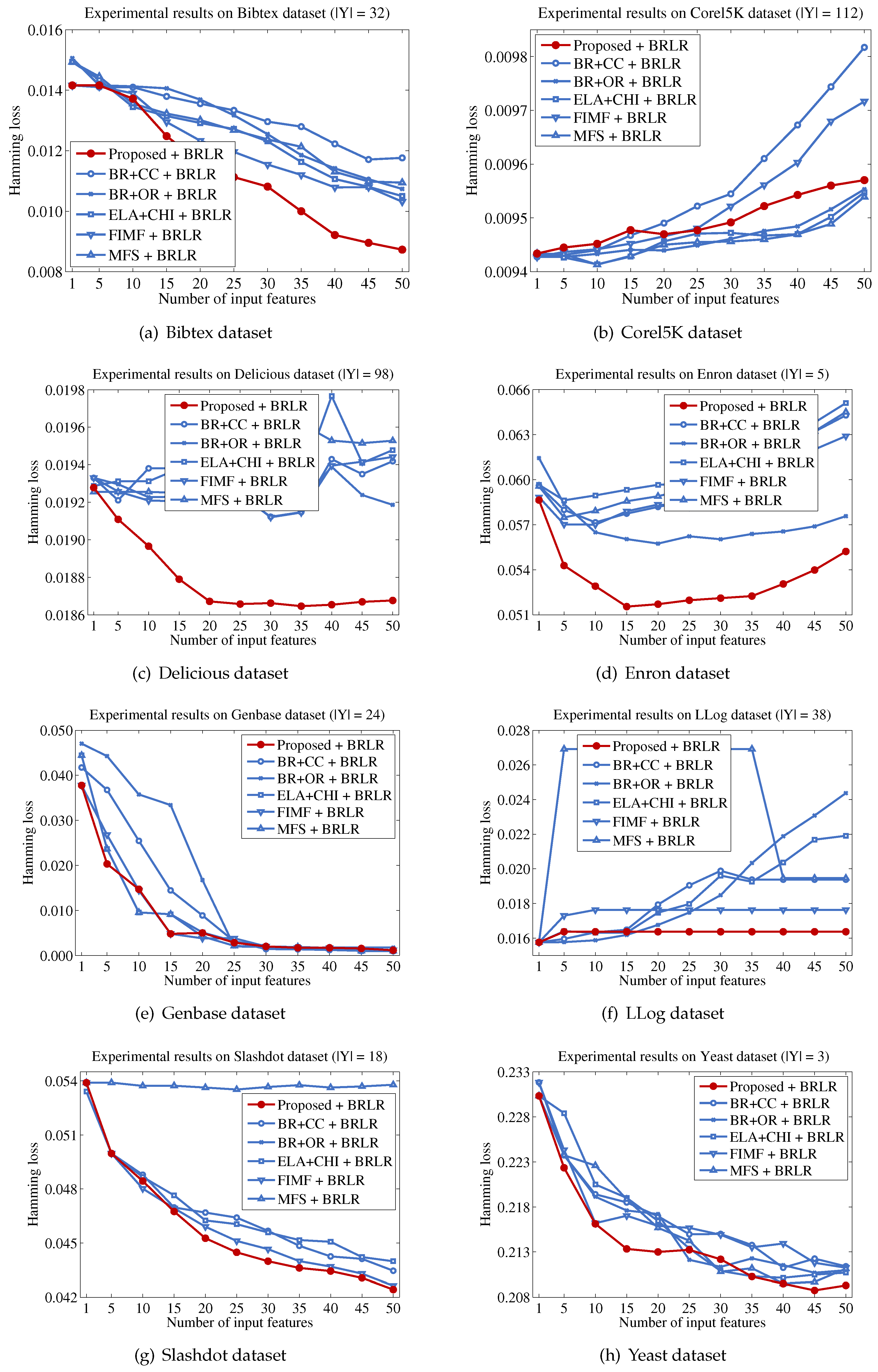
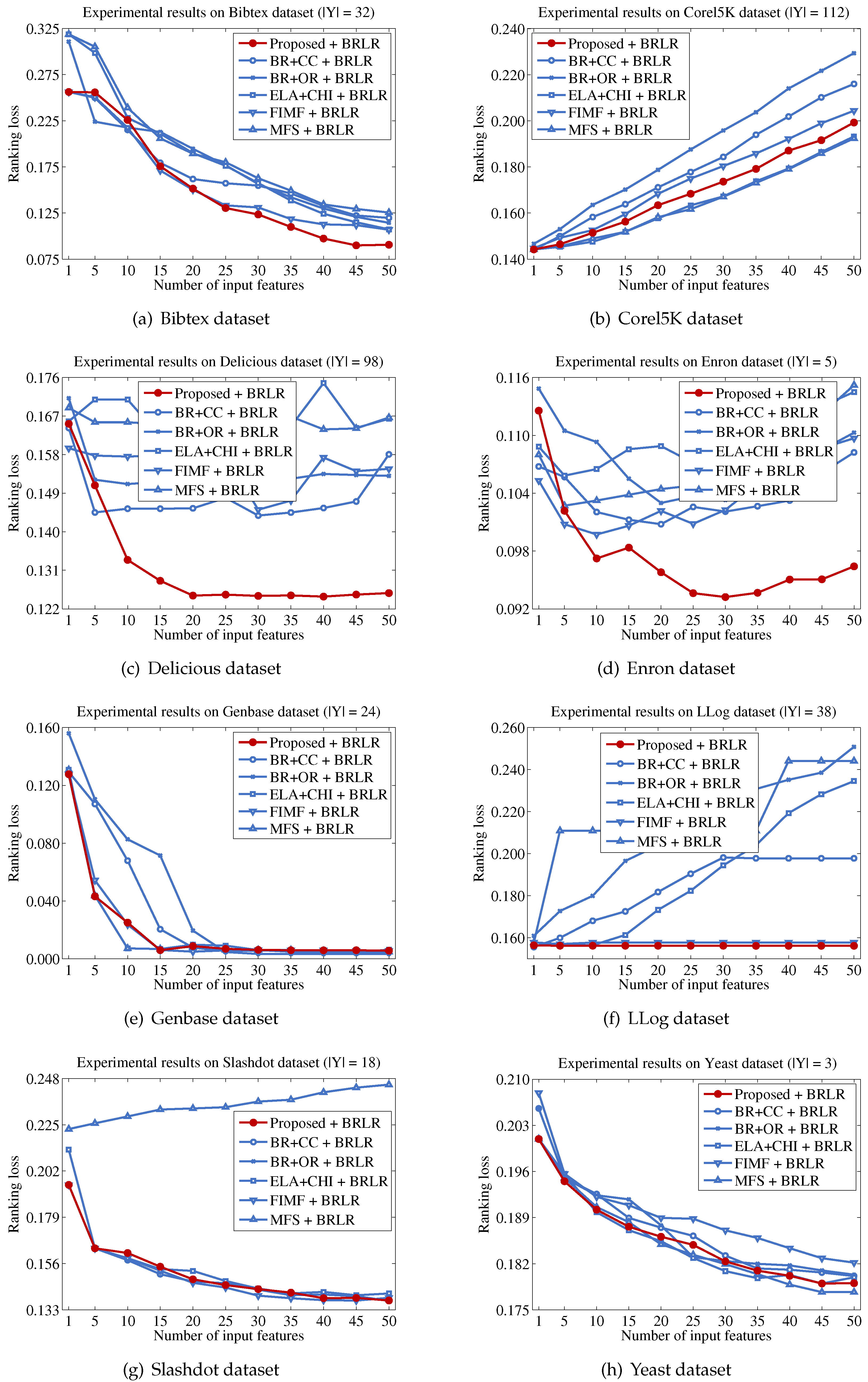
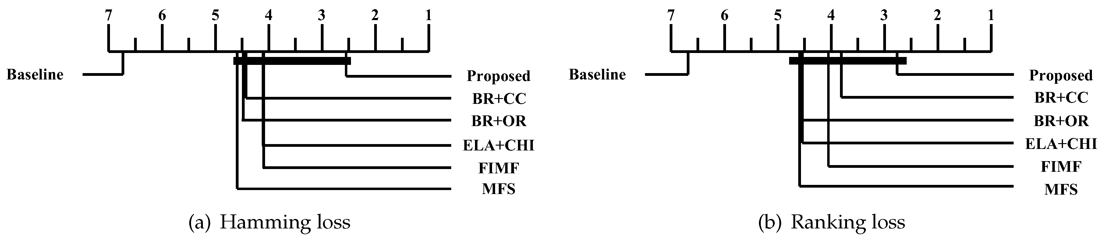
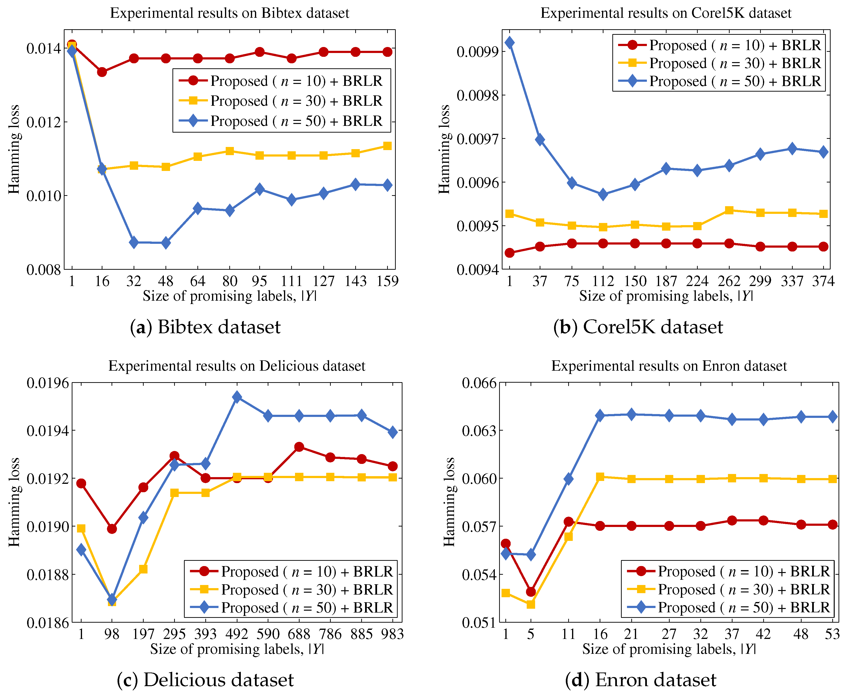
Finally, we describe the computational cost of the proposed method and compare this to a conventional binary relevance-based feature selection method, such as BR + CC, to show the efficiency of the proposed method. For a dataset with | W | patterns, | F | features and | L | labels, the time complexity of BR + CC can be written as O ( | W | · | F | · | L | ) , because it evaluates the Pearson correlation coefficient between each feature and each label and then aggregates those values to identify the features to be included in the final feature subset. Let us assume that the computational cost for computing mutual information and Pearson correlation coefficients is the same, as both operations commonly involve two variables and have to examine | W | patterns. Because the proposed method calculates the mutual information value between a feature and labels in Y, the computational cost for this process will be O ( | W | · | F | · | Y | ) . It should be noted that the calculation results for the entropy of each feature and each label are used to calculate mutual information terms, thus calculating K ( · , · ) terms does not increase the computational cost. Our analysis indicates that the computational cost of the proposed method will be significantly influenced by the size of the promising label set Y.

4. Experimental Results

4.1. Datasets and Experimental Settings

We conducted experiments related to the performance of the proposed method on eight multi-label datasets, composed of various numbers of labels [50,51]. Five datasets—Bibtex, Delicious, Enron, Language Log (LLog) and Slashdot—were obtained from the application of text categorization [10,11,12,30]; the Corel5K dataset was obtained from annotated images, each containing multiple objects [52]. Two datasets—Genbase and Yeast—were obtained by representing the multiple classes of biological functions [2,53]. These datasets have frequently been employed for the purpose of comparison in multi-label feature selection studies [15,18,35]. We discretized the Yeast dataset by using an equal-width interval scheme, in order to apply the feature selection methods [47]. Then, we mapped each numerical value into one of two bins. Table 1 presents the standard statistics for the multi-label datasets used in our experiments [10,54]. For a multi-label dataset U = { ( u i , λ i ) | 1 i | U | } , the label density can be defined as:
L D ( U ) = 1 | U | i = 1 | U | | λ i | | L |
where this indicates how many labels are assigned to a pattern, in the average portion against | L | . Thus, a smaller value for the label density indicates a higher sparsity for the given label set.
To test the performance of the proposed method from the viewpoint of computational efficiency, we choose five multi-label feature selection methods: BR + CC [37], BR + OR [38], ELA + CHI [25], FIMF [17] and MFS [28]. Two multi-label feature selection methods—BR + CC and BR + OR—perform the feature selection process based on the binary relevance-based problem transformation strategy. In this approach, the importance of each feature is determined by the sum of the Pearson’s correlation coefficient values or the odd ratio values between the features and labels. ELA + CHI avoids the need for additional efforts in considering the dependencies between labels, by encoding multiple labels into single labels. MF-Statistics (MFS) is chosen as a candidate because of its simple calculations for measuring feature contributions. FIMF reduces the computational cost for the multi-label feature scoring process by discarding unimportant variable subsets. To obtain the score for all features, we set the promising feature subset to F for FIMF. Superiority among multi-label feature selection methods is determined by comparing the execution times (in seconds) for obtaining the output feature subset.
The quality of a feature subset is measured in terms of the multi-label classification performance, based on feature subsets selected by each method. The size of the promising label set | Y | is identified by conducting a series of experiments (Section 4.2). We evaluate the performance of each method using the binary relevance-based logistic regressor (BRLR), owing to its strong capability for predicting binary outcomes that form the basis of a label set [55]. In particular, 80% of the randomly chosen patterns from the dataset are used in the training process, and the remaining 20% are used to measure the performance of each feature selection method [18]. Because the multi-label classification performance can differ depending on the number of input features, we measure the classification performance by changing the size from one to 50, with intervals of five features. The experiments were repeated ten times, and the multi-label classification performance is reported according to each evaluation measure. We considered two evaluation measures, which are employed in many multi-label learning studies: Hamming loss and ranking loss [10,18]. Let T = { ( t i , λ i ) | 1 i | T | } be a set of test patterns where λ i is a true label set for t i and is unknown to the multi-label classifier, resulting in U = W T and W T = . For each test pattern t i , a classifier such as BRLR will output a set of confidence values ψ i = { ψ i , 1 , , ψ i , | L | } for each label l L after learning on the training set W. If a confidence value ψ i , l is larger than the predefined threshold value, such as 0.5, then the corresponding label l can be included in the predicted label subset Y i . Based on the ground truth λ i , confidence values ψ i and predicted label subset Y i , the multi-label classification performance can be measured according to each evaluation measure. In particular, the Hamming loss is defined as:
h l o s s ( T ) = 1 | T | i = 1 | T | 1 | L | | λ i Y i |
where ▵ denotes the symmetric difference between two sets. The ranking loss is defined as:
r l o s s ( T ) = 1 | T | i = 1 | T | | ( a , b ) | a λ i , b λ i ¯ , ψ i , a ψ i , b | | λ i | | λ i ¯ |
where λ i ¯ is a complementary set to λ i . The Hamming loss evaluates the number of times that a pattern-label pair is misclassified, and the ranking loss determines the ranking quality of different labels for each test pattern. The two evaluation measures both indicate a good classification performance for low values. All methods were carefully implemented in a MATLAB 8.2 programming environment and tested on an Intel Core i7-3930K (3.2 GHz) (Intel, Santa Clara, CA, USA) with 64 GB memory.

4.2. Determination of the Size of a Promising Label Set

In this study, the proposed method is able to output different feature subsets according to the size of promising label set | Y | . Because the quality of feature subsets can vary according to | Y | , we conducted a series of experiments to set the size of the promising label set for the proposed method. For clarity, we represent the classification performance according to n = 10, 30 and 50, where | Y | varies. For each parameter setting with regard to n and | Y | , the experiment is repeated ten times, and the average classification performance is reported.
Figure 2 illustrates the Hamming loss performance of the proposed method, with varying n and | Y | . In each figure, the horizontal and vertical axes represent the size of the promising label set Y and the corresponding Hamming loss value, respectively. Specifically, the lines with filled circles, rectangles and diamonds represent the Hamming loss performances for n = 10, 30 and 50, respectively. The experimental results indicate that the classification performance changes according to n and | Y | . In the experiments involving the Bibtex, Corel5K, Delicious, Enron, Yeast and LLog datasets, the results indicate that the Hamming loss performance improves steeply until 10%–20% of the labels are included in Y. It is interesting to note that the proposed method achieves a comparable or better Hamming loss performance when Y is composed of a much smaller number of labels than L. For example, Figure 2a shows that the Hamming loss performance improves until | Y | = 32 , which is approximately 20% of the given label set, and it is better than that of | Y | = | L | = 159 . Because a smaller size of Y will accelerate the proposed method, this indicates that the proposed method is able to quickly identify the final feature subset without significantly degrading the classification performance. For the Ranking loss experiments presented in Figure 3, a similar tendency can be observed. For example, in the experiments for the Bibtex dataset, the Ranking loss performance of | Y | = 32 is better than that of | Y | = | L | = 159 and does not change significantly after that. Overall, the experimental results all indicate that the feature subset quality can be maintained even though | Y | is set to a much smaller value than | L | . Based on our experiments, the size of the promising label set can be identified for each dataset. Table 2 presents the size of the promising label set | Y | for each dataset for the proposed method. In addition, we choose 50 as the default value for the number of input features n, because this achieves a better multi-label classification performance in most cases.

4.3. Comparison to Conventional Multi-Label Feature Selection Methods

Because our primary goal is to develop an efficient multi-label feature selection method, we conducted empirical experiments on multi-label datasets with respect to the execution time. Table 3 presents the execution times (in seconds) of multi-label feature selection methods for each dataset. The execution time of the fastest multi-label feature selection method is highlighted in boldface. The experimental results indicate that the proposed method outputs the selected feature subsets significantly faster than the other methods. For example, the proposed method outputs the feature subset 9.5-times faster than BR + CC, which is the second-best method for the experiments on the Delicious dataset.
After selecting a subset of features from the original feature set, the execution time of the later learning algorithm will be reduced. To illustrate this aspect, we represent the execution time of BRLR using both the original feature set and selected features when n is set to 50 in Table 4, because the execution time of the learning algorithm is not influenced by the quality of the selected features. The results show that BRLR requires a considerably lower execution time when 50 features are given, indicating the merit of feature selection with respect to the execution time of the learning method.
Next, we consider the multi-label learning accuracy, as indicated by the feature subset selected by each method. Figure 4 and Figure 5 illustrate the multi-label classification performance of each feature selection method for the eight datasets in terms of the Hamming loss and ranking loss. Here, the horizontal axis and vertical axis represent the number of input features and multi-label classification performance value, respectively. Although the proposed method requires a considerably lower execution time than the compared methods, the experimental results indicate that the feature subset selected by the proposed method provides a similar multi-label classification performance as that provided by the compared methods. Specifically, for the experiments involving the Bibtex, Genbase, Slashdot and Yeast datasets, as shown in Figure 4a,e,g,h, respectively, the Hamming loss values of the feature subsets selected by the six multi-label feature selection methods, including the proposed method, improve as the number of input features increases. In the experiments involving the Bibtex, Delicious and Enron datasets, as shown in Figure 4a,c,d, respectively, the feature subset selected by the proposed method yields a better multi-label classification performance compared to the feature subsets selected by the compared methods, even though the proposed method outputs the feature subset at least 5.0-, 9.5- and 11.0-times faster, respectively, than the other methods. Finally, in the experiments involving the Corel5K, Genbase, Slashdot and Yeast datasets, as shown in Figure 4b,e,g,h, respectively, the feature subset selected by the proposed method achieves a similar multi-label classification performance, despite consuming a lower execution time. Figure 5 illustrates the ranking loss performance of the feature subsets selected by each multi-label feature selection method. Again, the feature subset selected by the proposed method results in ranking loss values that are similar to or better than those produced by the compared methods.
Table 5 and Table 6 present the classification performance of each feature selection method when n = 50, as obtained from the experiments depicted in Figure 4 and Figure 5. To demonstrate the effect of feature selection on the multi-label classification, we also present the baseline classification performance, achieved when the original feature set is given to BRLR. The multi-label feature selection method that produces the best average classification performance value among seven values according to each dataset is highlighted in boldface. To conduct performance analysis among the comparing multi-label feature selection methods, the Friedman test is employed that is a widely-used statistical test for comparisons of multiple methods over a number of datasets [56]. Given k methods and N datasets, let r i j denote the rank of the j-th method on the i-th dataset (mean ranks are shared in the case of ties). Let R j = 1 N i = 1 N r i j denote the average rank for the j-th method, under the null hypothesis (i.e., all methods have equal performance); the following Friedman statistic F F will be distributed according to the F-distribution with k 1 numerator degrees of freedom and ( k 1 ) ( N 1 ) denominator degrees of freedom:
F F = ( N 1 ) χ F 2 N ( k 1 ) χ F 2 , where χ F 2 = 12 N k ( k + 1 ) j = 1 k R j 2 k ( k + 1 ) 2 4
Table 7 represents the Friedman statistics F F and the corresponding critical values on each evaluation metric. As shown in Table 7, at a significance level of α = 0.05, the null hypothesis of equal performance among the comparing algorithms is rejected in terms of each evaluation measure. Consequently, we need to proceed with certain post hoc tests to analyze the relative performance among the comparison methods [56]. As we are interested in whether the proposed method achieves similar performance against other methods even though it consumes lesser computational cost, the Bonferroni–Dunn test is employed [57]. Here, the difference between the average ranks of the proposed method and one comparing method is compared with the following critical difference (CD).
C D = q α k ( k + 1 ) 6 N
For the Bonferroni–Dunn test, we have q α = 2.638 at a significance level of α = 0.05 , and thus, CD = 2.849 (k = 7, N = 8). Accordingly, the performance between the proposed method and one comparison method is deemed to be statistically similar if their average ranks over all datasets within one CD. To visualize the relative performance of the proposed method and other methods, Figure 6 illustrates the CD diagrams on each evaluation measure, where the average rank of each method is marked along the axis where lower ranks are placed in the right-side [56]. In each subfigure, any comparison method whose average rank is within one CD to that of the proposed method is interconnected with a thick line. Otherwise, any algorithm not connected with the proposed method is considered to have significantly different performance between themselves. The experimental results show that the feature subset selected by the proposed method achieves a significantly better classification performance than the baseline, indicating that the proposed method is able to improve the classification performance. In addition, the feature subset selected by the proposed method gives similar classification performances to those of the compared methods. Because the proposed method consumes lower computational cost than the compared methods, this means the proposed method is able to identify the important feature subset quickly, without degrading the multi-label classification performance.

4.4. Comparison to Label Selection Strategy

In the proposed method, the promising label set is identified by choosing the labels with the largest entropies. To validate our label selection strategy, we implemented an opposing method, which chooses labels with the smallest entropies to compose Y. For this comparison method, we did not expect the classification performance to change significantly, because M ( f ; y ) K ( f , y ) H ( y ) , where y is the considered label, and thus, the final score of the features according to the number of considered labels will not significantly change. Figure 7 compares the Hamming loss performance results for the eight datasets, according to the label selection strategy. Each figure contains two lines, representing the Hamming loss performance for each label selection strategy. The line with the filled circles represents the Hamming loss performance of the proposed method, and that with the filled diamonds represents the performance of the comparison method, according to the number of selected labels. The experimental results indicate that the Hamming loss performance of the proposed method significantly outperforms the compared method, endorsing the validity of our label selection strategy. In contrast, the experimental results also show that the Hamming loss performance of the compared method did not change significantly, confirming our expectations. In the experiments regarding the ranking loss, shown in Figure 8, a similar tendency can be observed.

5. Conclusions

In this paper, we have proposed an efficient multi-label feature selection method, based on a novel entropy-based label selection strategy. The proposed method reduces the computational cost of evaluating the feature importance by calculating the exact dependencies between the features and the promising label set and approximating the dependencies for influential labels. The experimental results demonstrate that the proposed method can generate the feature subset quickly, without requiring an excessive execution time or incurring a significant degradation in discriminating capability, thus supporting the efficiency of the proposed method. Future research directions will include the investigation of the multi-label learning performance with respect to the label selection strategy. Our experiments indicate that the feature subset selected by the proposed method can possibly deliver a better discriminating capability, even though the size of the promising label set is smaller than that of the original label set. Thus, we would like to investigate this issue more deeply.

Acknowledgments

This research is supported by the Ministry of Culture, Sports and Tourism (MCST) and Korea Creative Content Agency (KOCCA) in the Culture Technology (CT) Research & Development Program 2016.

Author Contributions

Jaesung Lee proposed the idea in this paper, performed the experiments and wrote the paper. Dae-Won Kim conceived of and designed the experiments and analyzed the data. Both the authors have read and approved the final manuscript.

Conflicts of Interest

The authors declare no conflict of interest.

References

  1. Boutell, M.; Luo, J.; Shen, X.; Brown, C. Learning multi-label scene classification. Pattern Recognit. 2004, 37, 1757–1771. [Google Scholar] [CrossRef]
  2. Diplaris, S.; Tsoumakas, G.; Mitkas, P.; Vlahavas, I. Protein classification with multiple algorithms. Adv. Inf. 2005, 3746, 448–456. [Google Scholar]
  3. Rao, Y. Contextual Sentiment Topic Model for Adaptive Social Emotion Classification. IEEE Intell. Syst. 2016, 31, 41–47. [Google Scholar] [CrossRef]
  4. Trohidis, K.; Tsoumakas, G.; Kalliris, G.; Vlahavas, I. Multi-label classification of music into emotions. In Proceedings of the 9th International Conference of Music Information Retrieval, Philadelphia, PA, USA, 14–18 September 2008.
  5. Lee, J.; Kim, H.; Kim, N.R.; Lee, J.H. An approach for multi-label classification by directed acyclic graph with label correlation maximization. Inf. Sci. 2016, 351, 101–114. [Google Scholar] [CrossRef]
  6. Madjarov, G.; Kocev, D.; Gjorgjevikj, D.; Džeroski, S. An extensive experimental comparison of methods for multi-label learning. Pattern Recognit. 2012, 45, 3084–3104. [Google Scholar] [CrossRef]
  7. Sun, X.; Xu, J.; Jiang, C.; Feng, J.; Chen, S.S.; He, F. Extreme Learning Machine for Multi-Label Classification. Entropy 2016, 18, 225. [Google Scholar] [CrossRef]
  8. Xiang, Y.; Chen, Q.; Wang, X.; Qin, Y. Distant Supervision for Relation Extraction with Ranking-Based Methods. Entropy 2016, 18, 204. [Google Scholar] [CrossRef]
  9. Zhang, M.L.; Wu, L. LIFT: Multi-label learning with label-specific features. IEEE Trans. Pattern Anal. Mach. Intell. 2015, 37, 107–120. [Google Scholar] [CrossRef] [PubMed]
  10. Zhang, M.L.; Zhou, Z.H. A review on multi-label learning algorithms. IEEE Trans. Knowl. Data Eng. 2014, 26, 1819–1837. [Google Scholar] [CrossRef]
  11. Katakis, I.; Tsoumakas, G.; Vlahavas, I. Multilabel text classification for automated tag suggestion. In Proceedings of the ECML PKDD Discovery Challenge 2008, Antwerp, Belgium, 15 September 2008.
  12. Klimt, B.; Yang, Y. The Enron Corpus: A New Dataset for Email Classification Research. Lect. Notes Comput. Sci. 2004, 3201, 217–226. [Google Scholar]
  13. Gibaja, E.; Ventura, S. A tutorial on multilabel learning. ACM Comput. Surv. 2015, 47, 52. [Google Scholar] [CrossRef]
  14. Lee, J.; Kim, D.W. Mutual information-based multi-label feature selection using interaction information. Expert Syst. Appl. 2015, 42, 2013–2025. [Google Scholar] [CrossRef]
  15. Lin, Y.; Hu, Q.; Liu, J.; Duan, J. Multi-label feature selection based on max-dependency and min-redundancy. Neurocomputing 2015, 168, 92–103. [Google Scholar] [CrossRef]
  16. Spolaôr, N.; Monard, M.C.; Tsoumakas, G.; Lee, H.D. A systematic review of multi-label feature selection and a new method based on label construction. Neurocomputing 2016, 180, 3–15. [Google Scholar] [CrossRef]
  17. Lee, J.; Kim, D.W. Fast multi-label feature selection based on information-theoretic feature ranking. Pattern Recognit. 2015, 48, 2761–2771. [Google Scholar] [CrossRef]
  18. Lee, J.; Kim, D.W. Feature selection for multi-label classification using multivariate mutual information. Pattern Recognit. Lett. 2013, 34, 349–357. [Google Scholar] [CrossRef]
  19. Liu, H.; Motoda, H. Computational Methods of Feature Selection; CRC Press: Boca Raton, FL, USA, 2007. [Google Scholar]
  20. Fong, S.; Wong, R.; Vasilakos, A. Accelerated PSO swarm search feature selection for data stream mining big data. IEEE Trans. Serv. Comput. 2016, 9, 33–45. [Google Scholar] [CrossRef]
  21. Ghasemzadeh, H.; Amini, N.; Saeedi, R.; Sarrafzadeh, M. Power-aware computing in wearable sensor networks: An optimal feature selection. IEEE Trans. Mob. Comput. 2015, 14, 800–812. [Google Scholar] [CrossRef]
  22. Jurado, S.; Nebot, À.; Mugica, F.; Avellana, N. Hybrid methodologies for electricity load forecasting: Entropy-based feature selection with machine learning and soft computing techniques. Energy 2015, 86, 276–291. [Google Scholar] [CrossRef] [Green Version]
  23. Linder, T.; Arras, K.O. Real-time full-body human attribute classification in RGB-D using a tessellation boosting approach. In Proceedings of the 2015 IEEE/RSJ International Conference on Intelligent Robots and Systems, Hamburg, Germany, 28 September–2 October 2015.
  24. Wen, X.; Shao, L.; Fang, W.; Xue, Y. Efficient feature selection and classification for vehicle detection. IEEE Trans. Circuits Syst. Video Technol. 2015, 25, 508–517. [Google Scholar]
  25. Chen, W.; Yan, J.; Zhang, B.; Chen, Z.; Yang, Q. Document transformation for multi-label feature selection in text categorization. In Proceedings of the 7th IEEE International Conference on Data Mining (ICDM 2007), Omaha, Nebraska, 28–31 October 2007.
  26. Doquire, G.; Verleysen, M. Mutual information-based feature selection for multilabel classification. Neurocomputing 2013, 122, 148–155. [Google Scholar] [CrossRef]
  27. Gu, Q.; Li, Z.; Han, J. Correlated multi-label feature selection. In Proceedings of the 20th ACM international conference on Information and knowledge management, Glasgow, UK, 24–28 October 2011; pp. 1087–1096.
  28. Kong, D.; Ding, C.; Huang, H.; Zhao, H. Multi-label ReliefF and F-statistic feature selections for image annotation. In Proceedings of the 2012 IEEE Conference on Computer Vision and Pattern Recognition (CVPR), Providence, RI, USA, 16–21 June 2012.
  29. Nie, F.; Huang, H.; Cai, X.; Ding, C. Efficient and robust feature selection via joint l2,1-norms minimization. Adv. Neural Inf. Process. Syst. 2010, 23, 1813–1821. [Google Scholar]
  30. Lee, J.; Kim, D.W. Memetic feature selection algorithm for multi-label classification. Inf. Sci. 2015, 293, 80–96. [Google Scholar] [CrossRef]
  31. Zhang, M.L.; Peña, J.M.; Robles, V. Feature selection for multi-label naive Bayes classification. Inf. Sci. 2009, 179, 3218–3229. [Google Scholar] [CrossRef]
  32. Qian, B.; Davidson, I. Semi-Supervised Dimension Reduction for Multi-Label Classification. In Proceedings of the 24th AAAI Conference on Artificial Intelligence, Atlanta, GA, USA, 11–15 July 2010.
  33. Kong, X.; Yu, P. gMLC: A multi-label feature selection framework for graph classification. Knowl. Inf. Syst. 2012, 31, 281–305. [Google Scholar] [CrossRef]
  34. Spolaôr, N.; Cherman, E.A.; Monard, M.C.; Lee, H.D. A Comparison of Multi-label Feature Selection Methods using the Problem Transformation Approach. Electron. Notes Theor. Comput. Sci. 2013, 292, 135–151. [Google Scholar] [CrossRef]
  35. Reyes, O.; Morell, C.; Ventura, S. Scalable extensions of the ReliefF algorithm for weighting and selecting features on the multi-label learning context. Neurocomputing 2015, 161, 168–182. [Google Scholar] [CrossRef]
  36. Tsoumakas, G.; Katakis, I.; Vlahavas, I. Random k-labelsets for multilabel classification. IEEE Trans. Knowl. Data Eng. 2011, 23, 1079–1089. [Google Scholar] [CrossRef]
  37. Jungjit, S.; Michaelis, M.; Freitas, A.A.; Cinatl, J. Two extensions to multi-label correlation-based feature selection: A case study in bioinformatics. In Proceedings of the 2013 IEEE International Conference on Systems, Man, and Cybernetics (SMC), Manchester, UK, 13–16 October 2013.
  38. Chen, J.; Huang, H.; Tian, S.; Qu, Y. Feature selection for text classification with Naïve Bayes. Expert Syst. Appl. 2009, 36, 5432–5435. [Google Scholar] [CrossRef]
  39. Read, J. A pruned problem transformation method for multi-label classification. In Proceedings of the 2008 New Zealand Computer Science Research Student Conference, Christchurch, New Zealand, 14–18 April 2008.
  40. Robnik-Šikonja, M.; Kononenko, I. Theoretical and empirical analysis of ReliefF and RReliefF. Mach. Learn. 2003, 53, 23–69. [Google Scholar] [CrossRef]
  41. Sun, Y.; Wong, A.; Kamel, M. Classification of imbalanced data: A review. Int. J. Pattern Recognit. Artif. Intell. 2009, 23. [Google Scholar] [CrossRef]
  42. Ji, S.; Ye, J. Linear Dimensionality Reduction for Multi-label Classification. In Proceedings of the Twenty-First International Joint Conference on Artificial Intelligence (IJCAI-09), Pasadena, CA, USA, 11–17 July 2009.
  43. Lee, J.; Lim, H.; Kim, D.W. Approximating mutual information for multi-label feature selection. Electron. Lett. 2012, 48, 929–930. [Google Scholar] [CrossRef]
  44. Lim, H.; Lee, J.; Kim, D.W. Multi-Label Learning Using Mathematical Programming. IEICE Trans. Inf. Syst. 2015, 98, 197–200. [Google Scholar] [CrossRef]
  45. Lin, Y.; Hu, Q.; Liu, J.; Chen, J.; Duan, J. Multi-label feature selection based on neighborhood mutual information. Appl. Soft Comput. 2016, 38, 244–256. [Google Scholar] [CrossRef]
  46. Shannon, C. A mathematical theory of communication. ACM SIGMOBILE Mobile Comput. Commun. Rev. 2001, 5, 3–55. [Google Scholar] [CrossRef]
  47. Dougherty, J.; Kohavi, R.; Sahami, M. Supervised and unsupervised discretization of continuous features. In Proceedings of the the Twelfth International Conference on Machine Learning, Tahoe City, CA, USA, 9–12 July 1995.
  48. Peng, H.; Long, F.; Ding, C. Feature selection based on mutual information criteria of max-dependency, max-relevance, and min-redundancy. IEEE Trans. Pattern Anal. Mach. Intell. 2005, 27, 1226–1238. [Google Scholar] [CrossRef] [PubMed]
  49. Cover, T.M.; Thomas, J.A. Elements of Information Theory; Wiley: Hoboken, NJ, USA, 1991. [Google Scholar]
  50. Mulan: A Java Library for Multi-Label Learning. Available online: http://mulan.sourceforge.net/datasets-mlc.html (accessed on 14 November 2016).
  51. MEKA: A Multi-label Extension to WEKA. Available online: http://meka.sourceforge.net (accessed on 14 November 2016).
  52. Duygulu, P.; Barnard, K.; de Freitas, J.F.; Forsyth, D.A. Object recognition as machine translation: Learning a lexicon for a fixed image vocabulary. In Proceedings of the 7th European Conference on Computer Vision, Copenhagen, Denmark, 28–31 May 2002.
  53. Elisseeff, A.; Weston, J. A kernel method for multi-labelled classification. In Proceedings of the 2001 Neural nformation Processing Systems, Vancouver, BC, Canada, 3–8 December 2001.
  54. Tsoumakas, G.; Spyromitros-Xioufis, E.; Vilcek, J.; Vlahavas, I. Mulan: A java library for multi-label learning. J. Mach. Learn. Res. 2011, 12, 2411–2414. [Google Scholar]
  55. Cheng, W.; Hüllermeier, E. Combining instance-based learning and logistic regression for multilabel classification. Mach. Learn. 2009, 76, 211–225. [Google Scholar] [CrossRef]
  56. Demsar, J. Statistical comparions of cclassifier over multiple data sets. J. Mach. Learn. Res. 2006, 7, 1–30. [Google Scholar]
  57. Dunn, O.J. Multiple comparisons among means. J. Am. Stat. Assoc. 1961, 56, 52–64. [Google Scholar] [CrossRef]
Figure 1. Illustration of the proposed method with our label selection strategy.
Entropy 18 00405 g001
Figure 2. Hamming loss performance of eight datasets according to the size of promising labels | Y | while varying the number of input features n. BRLR, binary relevance-based logistic regressor. (a) Bibtex dataset; (b) Corel5K dataset; (c) Delicious dataset; (d) Enron dataset; (e) Genbase dataset; (f) LLog dataset; (g) Slashdot dataset; (h) Yeast dataset.
Entropy 18 00405 g002aEntropy 18 00405 g002b
Figure 3. Ranking loss performance of eight datasets according to the size of promising labels | Y | while varying the number of input features n. (a) Bibtex dataset; (b) Corel5K dataset; (c) Delicious dataset; (d) Enron dataset; (e) Genbase dataset; (f) LLog dataset; (g) Slashdot dataset; (h) Yeast dataset.
Entropy 18 00405 g003aEntropy 18 00405 g003b
Figure 4. Hamming loss performance of eight datasets according to the number of input features n. (a) Bibtex dataset; (b) Corel5K dataset; (c) Delicious dataset; (d) Enron dataset; (e) Genbase dataset; (f) LLog dataset; (g) Slashdot dataset; (h) Yeast dataset.
Entropy 18 00405 g004
Figure 5. Ranking loss performance of eight datasets according to the number of input features n. (a) Bibtex dataset; (b) Corel5K dataset; (c) Delicious dataset; (d) Enron dataset; (e) Genbase dataset; (f) LLog dataset; (g) Slashdot dataset; (h) Yeast dataset.
Entropy 18 00405 g005
Figure 6. Comparison of the proposed method against other methods with the Bonferroni–Dunn test. Methods connected with the proposed method in the critical difference (CD) diagram are considered to have statistically similar performance (significance level α = 0.05 ).
Entropy 18 00405 g006
Figure 7. Comparison results for the Hamming loss performance of eight datasets according to each label selection strategy. (a) Bibtex dataset; (b) Corel5K dataset; (c) Delicious dataset; (d) Enron dataset; (e) Genbase dataset; (f) LLog dataset; (g) Slashdot dataset; (h) Yeast dataset.
Entropy 18 00405 g007aEntropy 18 00405 g007b
Figure 8. Comparison results for the ranking loss performance of eight datasets according to each label selection strategy. (a) Bibtex dataset; (b) Corel5K dataset; (c) Delicious dataset; (d) Enron dataset; (e) Genbase dataset; (f) LLog dataset; (g) Slashdot dataset; (h) Yeast dataset.
Entropy 18 00405 g008aEntropy 18 00405 g008b
Table 1. Standard characteristics of multi-label datasets.
DatasetsDomainPatternsFeaturesLabels
NumberTypeNumberDensity
BibtexText73951836Nominal1590.015
Corel5KImage5000499Nominal3740.009
DeliciousText16,105500Nominal9830.019
EnronText17021001Nominal530.064
GenbaseBiology6621186Nominal270.046
Language Log (LLog)Text14601004Nominal750.001
SlashdotText37821079Nominal220.054
YeastBiology2417103Numeric140.303
Table 2. The size of promising label set | Y | according to each dataset determined by our experiments.
DatasetsBibtexCorel5KDeliciousEnronGenbaseLLogSlashdotYeast
| Y | 321129852438183
Table 3. Execution time (in seconds) of six comparison methods (Proposed, BR + CC, BR + OR, ELA + CHI, FIMF, and MFS). The best performance among six comparing methods on each dataset is highlighted as the bold face.
DatasetsProposedBR + CCBR + ORELA + CHIFIMFMFS
Bibtex6.936.7287.357.444.734.2
Corel5K4.918.0128.014.617.414.4
Delicious9.893.1800.1241.6101.6102.5
Enron0.23.419.29.23.62.2
Genbase0.71.67.81.72.10.9
LLog1.24.725.43.04.12.7
Slashdot1.32.013.37.75.11.7
Yeast0.00.10.71.70.30.1
Table 4. Execution time (in seconds) of BRLR using the original feature set and selected features (n = 50). The better performance on each dataset is highlighted as the bold face.
Feature SetBibtexCorel5KDeliciousEnronGenbaseLLogSlashdotYeast
Original29,555.34085.736,181.9430.24.0429.4492.41.0
n = 5086.6144.41121.83.31.52.07.10.2
Table 5. Hamming loss performance of each multi-label feature selection method when n = 50. The best performance among six comparing methods on each dataset is highlighted as the bold face.
DatasetsBaselineProposedBR + CCBR + ORELA + CHIFIMFMFS
Bibtex0.0290.0090.0120.0110.0110.0100.011
Corel5K0.0180.0100.0100.0100.0100.0100.010
Delicious0.0280.0190.0190.0190.0190.0190.020
Enron0.1650.0550.0640.0580.0650.0630.065
Genbase0.0010.0010.0010.0020.0010.0010.001
LLog0.0970.0160.0190.0240.0220.0180.019
Slashdot0.0700.0420.0430.0540.0440.0430.054
Yeast0.2160.2090.2110.2110.2110.2110.211
Table 6. Ranking loss performance of each multi-label feature selection method when n = 50. The best performance among six comparing methods on each dataset is highlighted as the bold face.
DatasetsBaselineProposedBR + CCBR + ORELA + CHIFIMFMFS
Bibtex0.9660.0910.1200.1140.1070.1070.125
Corel5K0.5460.1990.2160.2290.1930.2040.192
Delicious0.2480.1260.1580.1530.1660.1550.167
Enron0.4780.0960.1080.1100.1140.1100.115
Genbase0.0050.0060.0040.0030.0060.0060.005
LLog0.5240.1560.1980.2510.2350.1580.244
Slashdot0.3930.1380.1370.2450.1410.1390.245
Yeast0.1840.1790.1800.1800.1800.1820.178
Table 7. Summary of the Friedman statistics F F (k = 7, N = 8) and the critical value in terms of each evaluation measure.
Evaluation Measure F F Critical Value (α = 0.05)
Hamming loss5.5062.324
Ranking loss4.8682.324

