Metrics and Energy Landscapes in Irreversible Thermodynamics

Abstract

We describe how several metrics are possible in thermodynamic state space but that only one, Weinhold’s, has achieved widespread use. Lengths calculated based on this metric have been used to bound dissipation in finite-time (irreversible) processes be they continuous or discrete, and described in the energy picture or the entropy picture. Examples are provided from thermodynamics of heat conversion processes as well as chemical reactions. Even losses in economics can be bounded using a thermodynamic type metric. An essential foundation for the metric is a complete equation of state including all extensive variables of the system; examples are given. Finally, the second law of thermodynamics imposes convexity on any equation of state, be it analytical or empirical.

1. Introduction

Geometry, and with that metrics, have been widely used in physics, where an intuitive understanding of the geometric object is often straight forward, e.g., in mechanics. At other times understanding the metric requires a bit of reflection, such as what it means that the fourth dimension, time, in relativistic Minkowski space is imaginary: $ict$. In thermodynamics, however, assigning an intuitively understandable metric with useful properties has been much harder, because when are two thermodynamic states close and how can their difference be quantified?

In the following we look at a very fruitful definition of thermodynamic length with several examples of how it can be used to bound dissipation in irreversible processes from a wide variety of topics. Next we use the requirement of the second law to derive fundamental restrictions on empirical equations of state, and thus the energy landscapes (equilibrium manifolds), on which the metric is defined.

2. Thermodynamic Length

Weinhold [1] was the first to rigorously define a metric on the thermodynamic state space of all extensive variables. He found that

$${\mathbf{M}}_U=\frac{d^{2}U}{d\mathbf{X}d\mathbf{X}},$$

(1)

where U is the internal energy of the system and $\mathbf{X}$ are all the other extensive variables $\{S,V,n_1,n_2,\cdots \}$ (entropy, volume, particle number, etc.), has all the properties required of a metric. However, traditionally this second derivative has been associated with the curvature of the surface of equilibrium states and its convexity ensures the second law of thermodynamics. Those two interpretations of the second derivative conflict. The second derivative cannot have both meanings at the same time. In the Gibbs view the equilibrium surface is defined through the equation of state, $f(U,S,V,n_1,n_2,\cdots )=0$ in the $n+1$ dimensional space $\{U,S,V,n_1,n_2,\cdots \}$ of all the n independent extensive variables plus the chosen dependent one (typically U or S). In this picture the curvature of the equilibrium surface is inherited from the $n+1$ dimensional space in which it is embedded. By contrast, Weinhold used the second derivative as a metric on the tangent space of the equation of state surface, converting it to an inner-product space and necessitating abandoning the picture of a convex surface. This led to a controversy about the “right” metric [2,3], but nowadays Equation (1) is consistently used as the metric of choice, not least due to its useful derived properties, of which some are described below. This does not rule out using the convexity requirement of the equilibrium surface to ensure the second law in a separate argument.

Surprisingly, Weinhold’s purpose was not to explore the thermodynamic geometric space, but to facilitate students writing down all the partial derivatives of the Maxwell relations using an analogy to the well known bra-ket notation of quantum mechanics. This idea did not catch on, but the metric was established and it was quickly picked up by others [4] and used to explore the full thermodynamic state space, in particular the meaning of lengths calculated with this metric. This development took off when it was discovered that these lengths can be used to bound dissipation in irreversible processes [5].

Using Weinhold’s metric Equation (1) one can calculate the length of a specified path (e.g., adiabatic or isothermal) as

$$L={\int }_{\text{process}\text{path}}\sqrt{d\mathbf{X}{\mathbf{M}}_{U}d\mathbf{X}}.$$

(2)

This length in turn can be used to bound the lost exergy (availability) of the specified path,

$$\Delta A\ge \frac{L^2\epsilon }{\tau }.$$

(3)

Here, τ is the duration of the process and ε the internal relaxation time of the system. Equality is achieved when the thermodynamic speed $dL/dt$ is constant throughout the process. A similar expression was derived for the entropy metric ${\mathbf{M}}_S=-d^{2}S/d\mathbf{X}d\mathbf{X}$, bounding the entropy production in the process [6]. Actually, Ruppeiner [7] used this entropy metric to extend fluctuation theory to regions smaller than the correlation length, even before its equivalence to the energy metric was established. Other interpretations of lengths of paths are the number of distinguishable states between the endpoints [7] and the number of states that can be distinguished by a certain measuring apparatus [8]. Also, systems described statistically through their state probabilities $p_i$ can be analyzed this way [9] using the very simple diagonal metric ${\mathbf{M}}_S=-[1/p_i]$. For processes proceeding in steps from one equilibrium state to another, dissipation is bounded by

$$\Delta S\ge \frac{L^2}{2K},$$

(4)

where K is the number of steps in the process. Here, equality is achieved when all steps have the same length, $L/K$.

The traditional equilibrium thermodynamic version of Equation (3) is simply

$$\Delta A\ge 0,$$

(5)

or equivalently

$$\overline{W}\ge \Delta F,$$

(6)

where W is the work performed on the system, the overbar indicates average over an ensemble of occurrences, and $\Delta F$ is the change of Helmholtz free energy of the system for the specified process, i.e., usually a constant. In either case, these equations only state that some losses appear at non-vanishing speed, while Equation (3) provides a stricter positive lower bound on the losses. More recently, Jarzynski [10] turned these bounds into an equality,

$$\overline{exp(-\beta W)}=exp(-\beta \Delta F),$$

(7)

where $\beta =1/kT$. This derivation contains two important improvements: It is an equality, not merely a bound; and it is true for any duration τ and for any process path. All the dynamics is hidden in the ensemble average which will, of course, depend on which path is followed and how far the process was from equilibrium, i.e., the process duration.

While this last equation did not use length explicitly, work is still continuing on deriving thermodynamic length from measurements and on comparing bounds like Equation (3) to a number of other divergence measures [11].

Whereas most systems have a paraboloid looking energy surface with a positive curvature from which to calculate the metric ${\mathbf{M}}_U$ (or equivalently inverted paraboloid if working in entropy space), situations do occur where the metric is zero, resulting in a length of zero and thus a vanishing minimum dissipation Equation (3). The prime example of such zero-length directions is a phase change, but other transformations which can take place without dissipation also exist, e.g., chemical reactions. The flatness of the energy surface is simply indicative of scaling the system—one component disappears while another emerges. No dissipation occurs here. Only dissipative reactions or transformations give rise to curvature and thus a thermodynamic length.

The starting point for calculating a thermodynamic metric is always the full equation of state for the system in question. For a simple ideal gas with just two degrees of freedom it is usually stated as

$$U(S,V)=b{e}^{S/C_v}{V}^{-k/C_v}$$

(8)

in the energy picture or

$$S(U,V)=C_{v}lnU+klnV+a$$

(9)

in the entropy picture (a and b are constants). These give rise to the two metrics

$${\mathbf{M}}_U=\left(\begin{array}{cc}\frac{{\partial }^{2}U}{\partial S^2}& \frac{{\partial }^{2}U}{\partial S\partial V}\\ \frac{{\partial }^{2}U}{\partial V\partial S}& \frac{{\partial }^{2}U}{\partial V^2}\end{array}\right)=\left(\begin{array}{cc}\frac{T}{C_v}& \frac{-P}{C_v}\\ \frac{-P}{C_v}& \left(1+\frac{k}{C_v}\right)\frac{P}{V}\end{array}\right)$$

(10)

and

$${\mathbf{M}}_S=\left(\begin{array}{cc}\frac{{\partial }^{2}S}{\partial U^2}& \frac{{\partial }^{2}S}{\partial U\partial V}\\ \frac{{\partial }^{2}S}{\partial V\partial U}& \frac{{\partial }^{2}S}{\partial V^2}\end{array}\right)=\left(\begin{array}{cc}\frac{C_v}{U^2}& 0\\ 0& \frac{k}{V^2}\end{array}\right).$$

(11)

As is apparent, they are made up of quite normal thermodynamic quantities. For the ideal gas the entropy metric is even conveniently diagonal.

If we also introduce quantities of material $n_i$ so that we may describe chemical reactions, the equation of state becomes considerably more complicated [12]:

$$U(S,V,\left\{n_i\right\})=b{e}^{\frac{S}{N{C}_v}}N\prod _i{\left[{\left(\frac{n_i}{V}\right)}^{\frac{k}{C_v}}\frac{1}{m_i}\right]}^{\frac{n_i}{N}}.$$

(12)

Here N is the total amount of material, $N={\sum }_i{n}_i$, and $m_i$ is the mass of particle type i. This is the unifying form of the more well known partial equations of state, $PV=NRT$, $U=C_{v}T$, and ${\mu }_i=kT[ln(n_i/V)-(C_v/k)ln\left(m_{i}kT\right)+a]$, each one a projection of Equation (12) keeping certain parameters fixed. However, the length calculations require the full form. For a mixture of ideal gases we then find the full metric

$$\begin{array}{cc}\hfill {\mathbf{M}}_U& =\left(\begin{array}{ccc}\frac{{\partial }^{2}U}{\partial S^2}& \frac{{\partial }^{2}U}{\partial S\partial V}& \frac{{\partial }^{2}U}{\partial S\partial n_i}\\ \frac{{\partial }^{2}U}{\partial V\partial S}& \frac{{\partial }^{2}U}{\partial V^2}& \frac{{\partial }^{2}U}{\partial V\partial n_i}\\ \frac{{\partial }^{2}U}{\partial n_j\partial S}& \frac{{\partial }^{2}U}{\partial n_j\partial V}& \frac{{\partial }^{2}U}{\partial n_j\partial n_i}\end{array}\right)\hfill \\ & =\left(\begin{array}{ccc}\frac{T}{N{C}_v}& \frac{-P}{N{C}_v}& \frac{{\mu }_i}{N{C}_v}-\frac{T}{N}\\ \frac{-P}{N{C}_v}& \left(1+\frac{k}{C_v}\right)\frac{P}{V}& -\frac{k}{C_v}\frac{{\mu }_i}{V}\\ \frac{{\mu }_j}{N{C}_v}-\frac{T}{N}& -\frac{k}{C_v}\frac{{\mu }_j}{V}& {\mu }_i\left(\frac{{\mu }_j}{U}-\frac{1}{N}\right)-\frac{1}{N}{\mu }_j+\frac{1}{N^2}U+\frac{RT}{n_j}{\delta }_{ij}\end{array}\right).\hfill \end{array}$$

(13)

The last row and column are really a condensed notation for all the participating particles i or j, and ${\delta }_{ij}$ is the Kronecker delta, meaning that the term only appears in the diagonal of the metric.

Immediate applications of this geometry to distillation and sequential chemical reactions are described in the next two sections, and extensions into economics in the subsequent section.

Further geometrizations of thermodynamics with different definitions have proven useful in many contexts like black holes [13,14], material behavior [15], fluctuations [16], and basic thermodynamic theory [17] just to point to a few.

3. Distillation

As a first example of geometric optimization, let us look at trayed distillation. It is a very common unit process in chemical engineering, but unfortunately it is thermodynamically quite inefficient. Even under the very best of conditions, separating an ideal 50–50 mixture into its two components using an ideal distillation column of infinite length, the thermodynamic efficiency cannot exceed 69%. In real life it is much lower. The main problem lies in the construction of the distillation column itself: All heat is added at the bottom of the column and all heat is withdrawn at the top, thus being degraded over the full temperature span of the column, even though the largest heat demand is only in the middle around the feed point. Improvement can only be achieved with additional control of the process, requiring in turn more freedom in its construction. The obvious extension is to allow heat to be added and withdrawn on any tray in the column as the optimization may require. The concept of such diabatic distillation columns is not new (see e.g., [18,19,20]), the novelty is calculating the optimal heat distribution, which is where thermodynamic length comes in.

This geometric method actually applies to a wide variety of conversion and transport processes [21].

A trayed distillation column is a step process where liquid and gas are in equilibrium on the K trays whereas the space between the trays is beyond our control. Thus we can calculate the thermodynamic distance L from top to bottom of this column from the specified purity of the light and the heavy products, and arrive at the dissipation bound Equation (4). As stated in the previous section, the least dissipative path will be the one where all the steps are of the same thermodynamic length, $L/K$. The final component is to calculate backwards from thermodynamic length to e.g., temperature of the mixture on each tray.

On each tray of the distillation column, the energy of the mixture is a function of a large number of extensive variables: Volume, entropy, amount of light component, and amount of heavy component, all for the liquid as well as the vapor phase, i.e., 8 variables, making the metric matrix from Equation (1) $8\times 8$. Fortunately, a number of conservation equations can reduce that number dramatically. E.g., we have mass conservation of both components, the column typically operates under constant pressure, and we have equilibrium between the gas and liquid phases on the trays. All combined these constraints reduce the number of degrees of freedom to one, which for simplicity we may take to be the temperature on each tray [22].

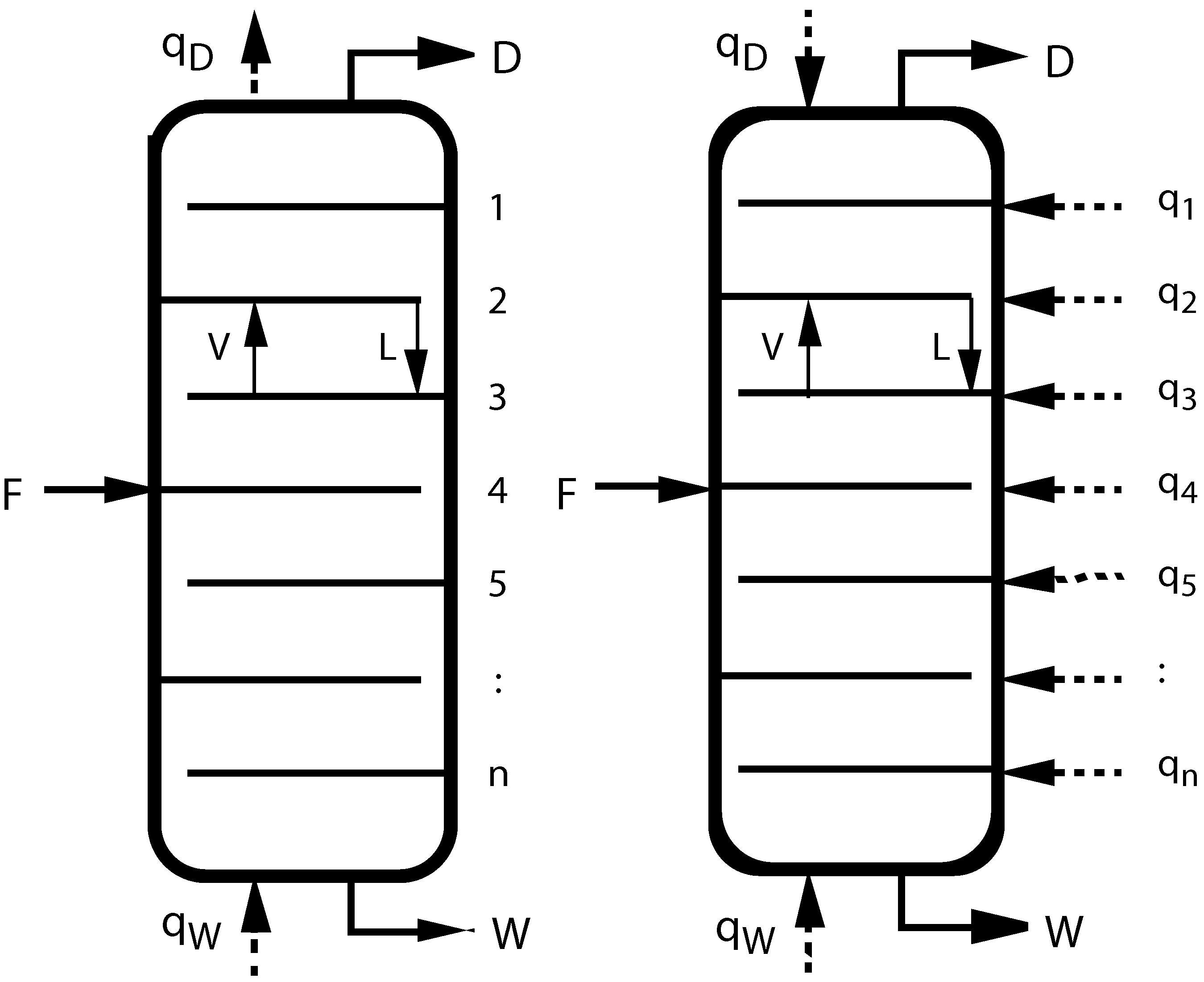
The example chosen to illustrate optimal distillation is the separation of an ideal 50–50 mixture of benzene and toluene into almost pure components in a 72 tray column. This diabatic column is compared in Figure 1 with a conventional adiabatic distillation column. The absolute best operation, concentrating only on the distillation process itself without worrying about how heat gets into and out of the fluid, reduces the exergy demand of this separation by a factor of 4 compared to the usual adiabatic operation [22]. 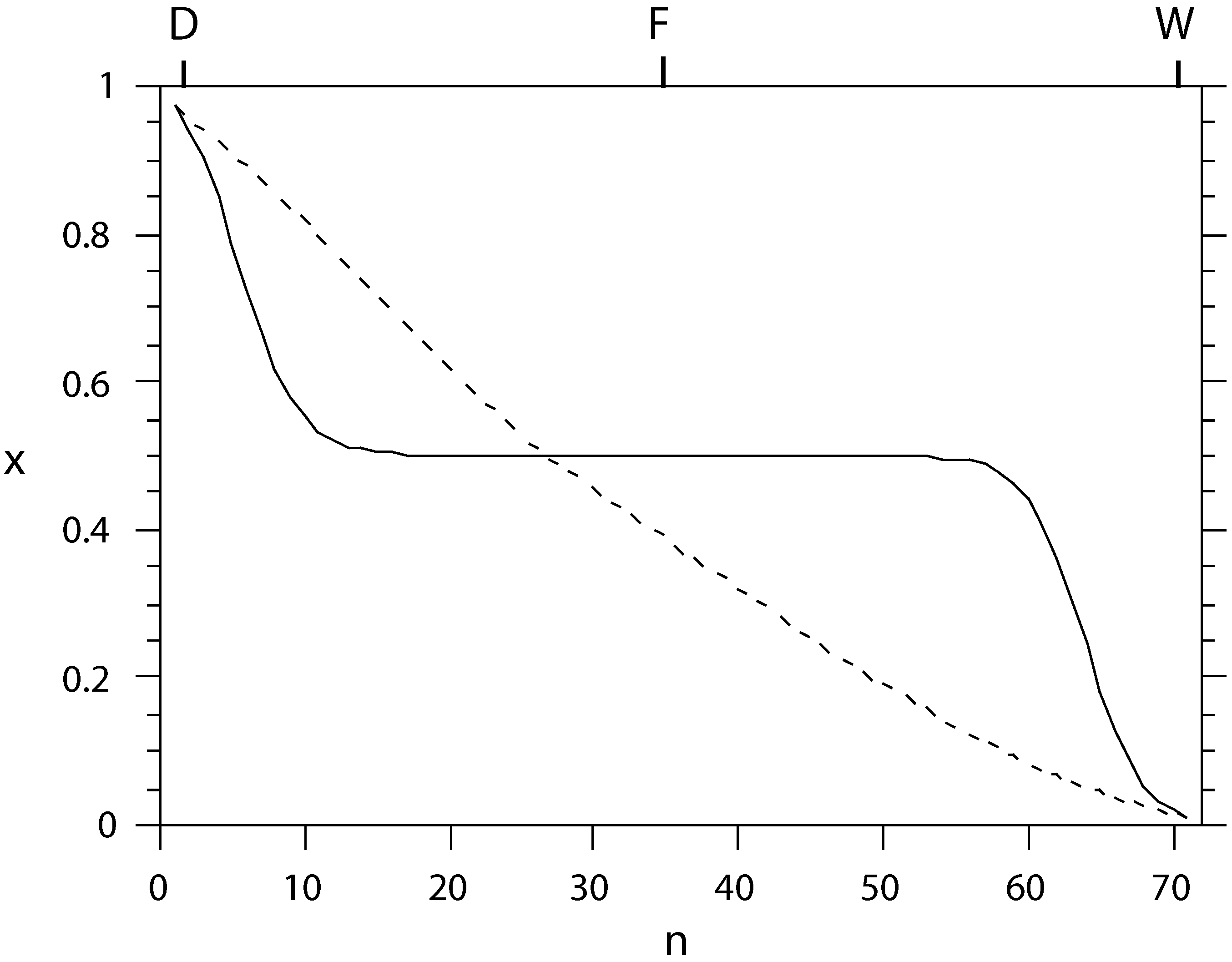Actually, allowing the number of trays in the column to go to infinity, the thermal separation efficiency approaches 1, i.e., reversible separation. The physical reason for this is that while energy and mass conservation between trays force large temperature steps around the feed point for a conventional column, the freedom to adjust the tray temperatures individually in the optimal diabatic column can split the burden of separation evenly among all trays, making it go to zero as the number of trays approaches infinity, as illustrated in Figure 2.

Figure 1. (left) Sketch of a conventional adiabatic distillation column with feed, distillate, and waste (bottoms) rates F, D, W, heating and cooling rates $q_W$ and $q_D$, and tray numbers n. V and L inside the columns indicate vapor and liquid flow rates between trays; (right) Sketch of a diabatic distillation column with heating or cooling on all trays.

Figure 1. (left) Sketch of a conventional adiabatic distillation column with feed, distillate, and waste (bottoms) rates F, D, W, heating and cooling rates $q_W$ and $q_D$, and tray numbers n. V and L inside the columns indicate vapor and liquid flow rates between trays; (right) Sketch of a diabatic distillation column with heating or cooling on all trays.

Figure 2. The liquid composition profile x (mole fraction of light component) as a function of tray number n, counted from the condenser, for conventional (solid) and equal-thermodynamic-distance (dashed) separation of an ideal benzene-toluene system. The separation effort is almost equally distributed among the trays in the latter setup.

Figure 2. The liquid composition profile x (mole fraction of light component) as a function of tray number n, counted from the condenser, for conventional (solid) and equal-thermodynamic-distance (dashed) separation of an ideal benzene-toluene system. The separation effort is almost equally distributed among the trays in the latter setup.

4. The Cytochrome Chain

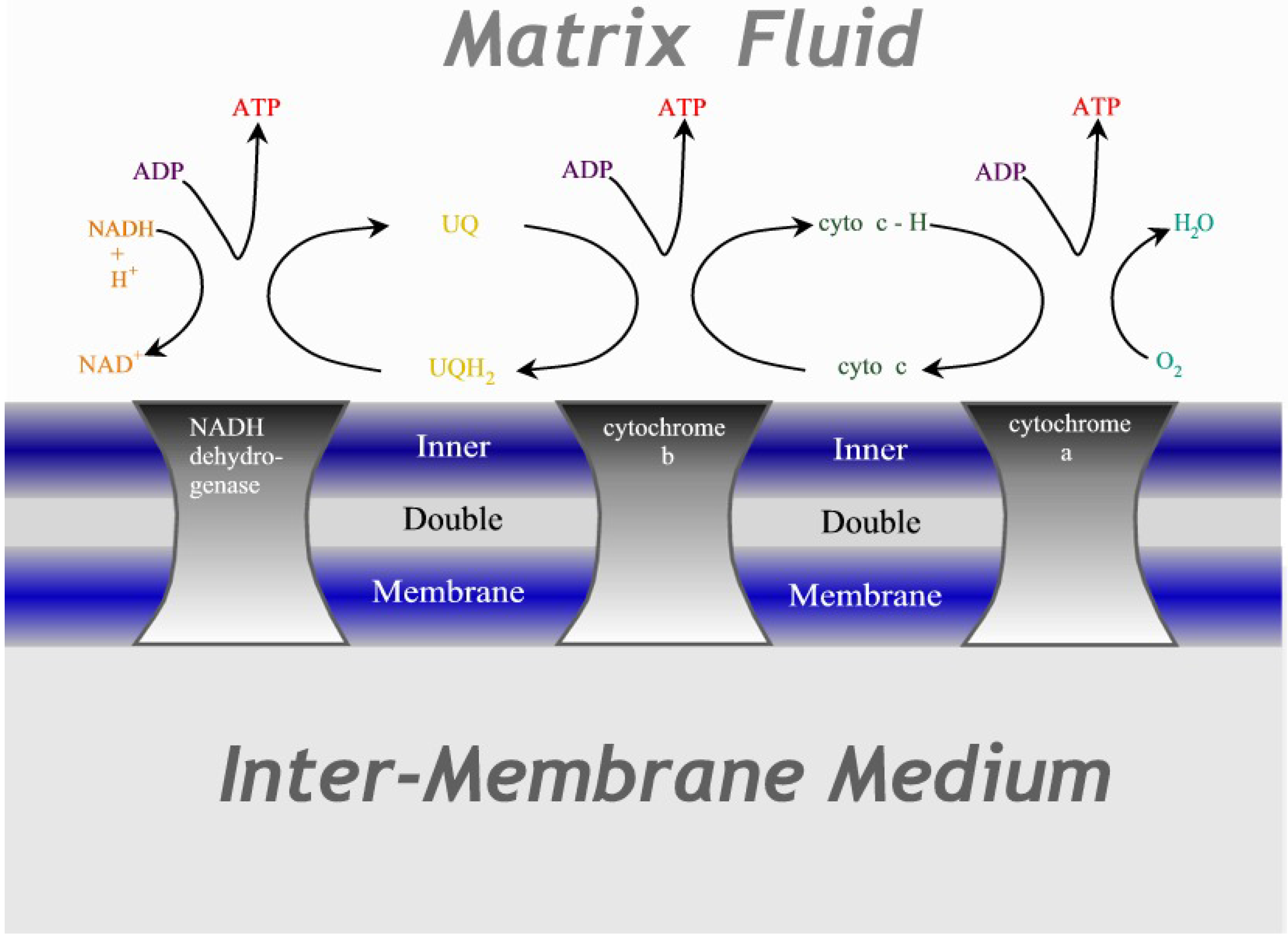
As our second example of thermodynamic geometric optimization we take the cytochrome chain, which has recently been optimized for maximum conversion of chemical energy from hydrogen into the carrier ATP [23]. This is the primary energy source in mitochondria, where essentially all hydrogen from the food of the cell passes through this three-step reaction to combine with oxygen to form water, as shown in Figure 3. The technical equivalent is a fuel cell where the reaction $H_2+\frac{1}{2}{O}_2\rightleftharpoons H_{2}O$ proceeds in a single chemical step while producing electrical power.

Figure 3. Illustration of the cytochrome chain. Three protein complexes embedded in the inner mitochondrial double membrane act as catalysts for the redox reactions, transferring electrons in successive steps through ubiquinone and cytochrome-c before terminating as water.

Figure 3. Illustration of the cytochrome chain. Three protein complexes embedded in the inner mitochondrial double membrane act as catalysts for the redox reactions, transferring electrons in successive steps through ubiquinone and cytochrome-c before terminating as water.

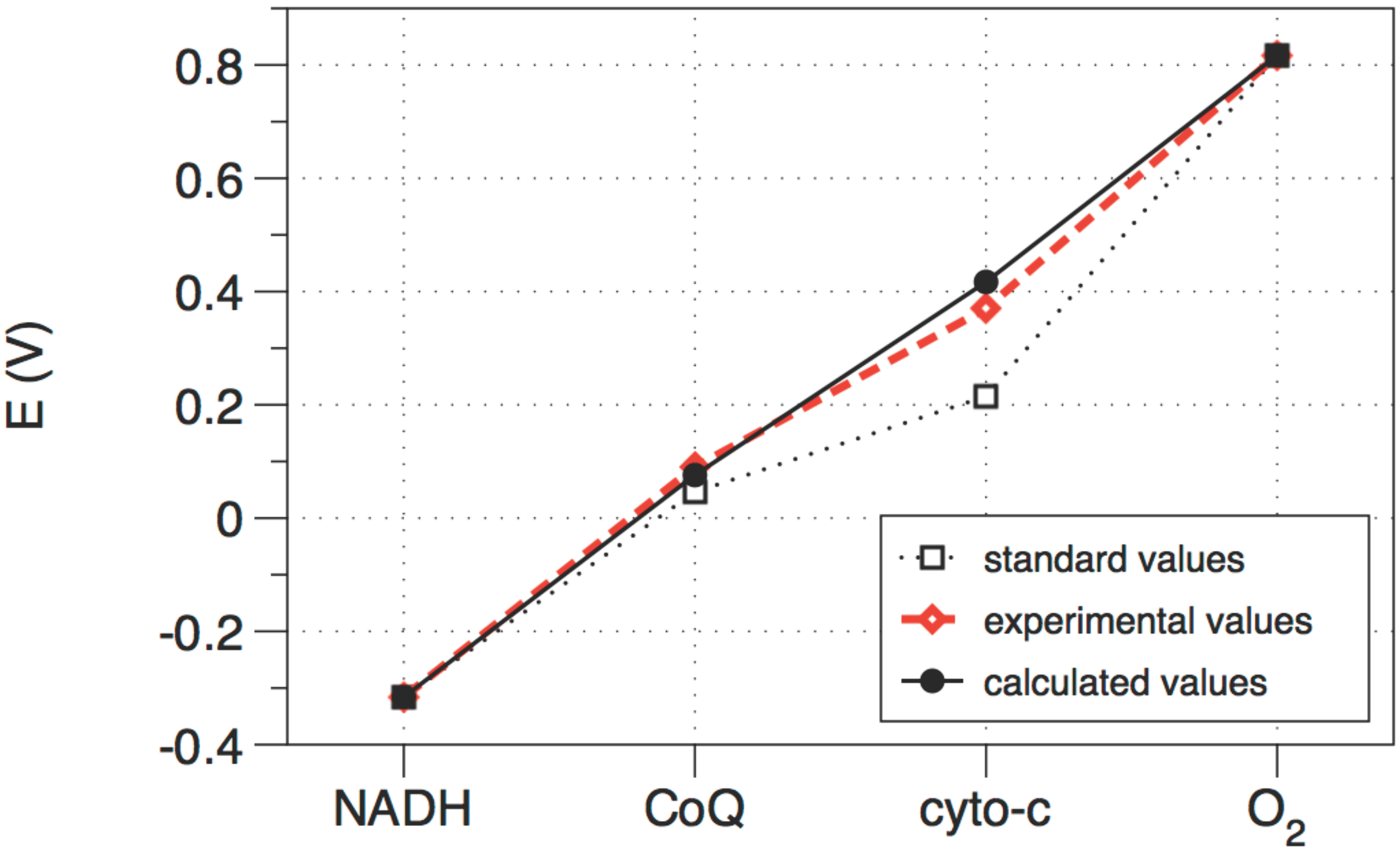
The analytical solution of the cytochrome chain treated as a step process proceeds as described for distillation above, i.e., by setting up the full equation of state, calculating the metric, and reducing the dimensionality of the problem using all available constraints. Again, the problem reduces to a single degree of freedom, which is most conveniently taken to be the electrochemical potential at points along the path. This yields the optimal path shown in Figure 4, which is very close to the path actually taken by the cytochrome chain inside a real mitochondrion. Thus mitochondria are well optimized for efficient power production.

The take home lesson is that finite-time thermodynamics optimization using thermodynamic length is indeed very descriptive of real systems. A recent review of finite-time thermodynamics, geometric and otherwise, may be found in [24].

Figure 4. The standard (i.e., not corrected for concentration), calculated (optimized), and observed values of the electrochemical potential of each electron transfer unit in the cytochrome chain. The three redox steps are almost equal.

Figure 4. The standard (i.e., not corrected for concentration), calculated (optimized), and observed values of the electrochemical potential of each electron transfer unit in the cytochrome chain. The three redox steps are almost equal.

5. Economics

Next, let us look at the influence of geometric finite-time thermodynamic ideas outside the traditional realm of macroscopic thermodynamics. It was realized quite early that the thinking and methods of finite-time thermodynamics were also applicable in economic theory [25,26,27] in two distinct ways. In the first instance, the finite-time thermodynamics ideas could be directly transplanted to economics, simply changing the meaning of the variables such that the bounds on thermodynamic losses become bounds on economic losses. The case studied was the market situation where sellers and buyers are not equally up to date on the market conditions. This creates a loss, a foregone earning, which the buyers could have had if they had possessed the full information, much like lost work in an irreversible process. This time delay of information is akin to the relaxation time in a thermodynamic process and prices in the market are like temperatures in thermodynamics. With this analogy dissipation (foregone earning) is limited from below by the same formula, Equation (3), as in thermodynamics,

$$\text{foregone}\text{earning}\ge \frac{L^2}{\tau },$$

(14)

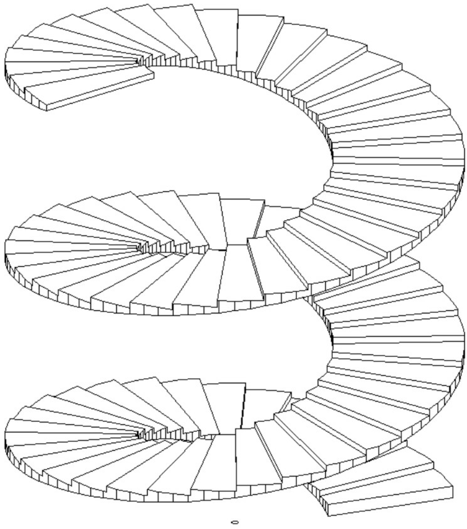
just with parameters taken from the economic universe rather than the thermodynamic one [26]. Now τ is the duration of the trade. For the widely used Cobb–Douglas utility function, $U(x,y)=x^a{y}^b$, e.g., the geometry is a spiral (see Figure 5) and thus flat in the corresponding circular coordinates $(r,\theta )$ with the length between points $(x_1,y_1)$ and $(x_2,y_2)$ given by

$$\begin{array}{cc}L((x_1,y_1),(x_2,y_2))=\sqrt{{(x_2-x_1)}^2+{(y_2-y_1)}^2}\hfill & \text{if}|{\theta }_2-{\theta }_1|\le \pi \hfill \\ L((x_1,y_1),(x_2,y_2))=\sqrt{x_1^2+y_1^2}+\sqrt{x_2^2+y_2^2}\hfill & \text{if}|{\theta }_2-{\theta }_1|>\pi .\hfill \end{array}$$

(15)

Figure 5. An illustration of the geometry of the set of the Cobb–Douglas utility function $U(x,y)=x^a{y}^b$. Locally, the surface is a plane while an infinite number of planes need to be spliced together for the entire surface.

Figure 5. An illustration of the geometry of the set of the Cobb–Douglas utility function $U(x,y)=x^a{y}^b$. Locally, the surface is a plane while an infinite number of planes need to be spliced together for the entire surface.

Related to this extrapolation into economic thinking, but still within the physical world, is the economic optimization of a heat engine, i.e., maximizing the profit while selling the power (electricity) and buying the heat (coal) [28,29]. A more elaborate optimization, taking into account both operating and investment costs, is under way [30]. Tsirlin and his group have also recognized this systemic similarity between thermodynamics and economics. In [31] they review this one-to-one relationship, and in particular define irreversibility and temperature in economic terms.

6. Convexity and the Second Law

Any thermodynamic state on the equilibrium manifold of a thermodynamic system can be defined by a position vector, $\mathbf{r}=(U,S,V,n_1,n_2,\cdots )$ in extensity space, where $\mathbf{r}\in {\mathbb{R}}^{n+1}$. Here n is the number of independent variables of the extensity space, i.e., the number of arguments for $U(S,V,\left\{n_i\right\})$, Equation (12). Usually this equilibrium manifold is referred to as the energy landscape of the system, although other areas of thermodynamics use this expression for a slightly different set of independent variables. Of course, points not on the manifold can be similarly located, but only position vectors that fall on the manifold defined by Equation (12) constitute unconstrained equilibrium states. Locations off that surface can be reached mathematically by using the additivity of mutually independent equilibrium systems, although those points do not generally correspond to physically realizable states. An equilibrium state of a homogeneous system is fully represented by a position vector $\mathbf{r}$ rooted in the origin and ending on the surface. By virtue of the scaling property

$$\lambda U(S,V,n_1,n_2,\cdots )=U(\lambda S,\lambda V,\lambda n_1,\lambda n_2,\cdots )$$

(16)

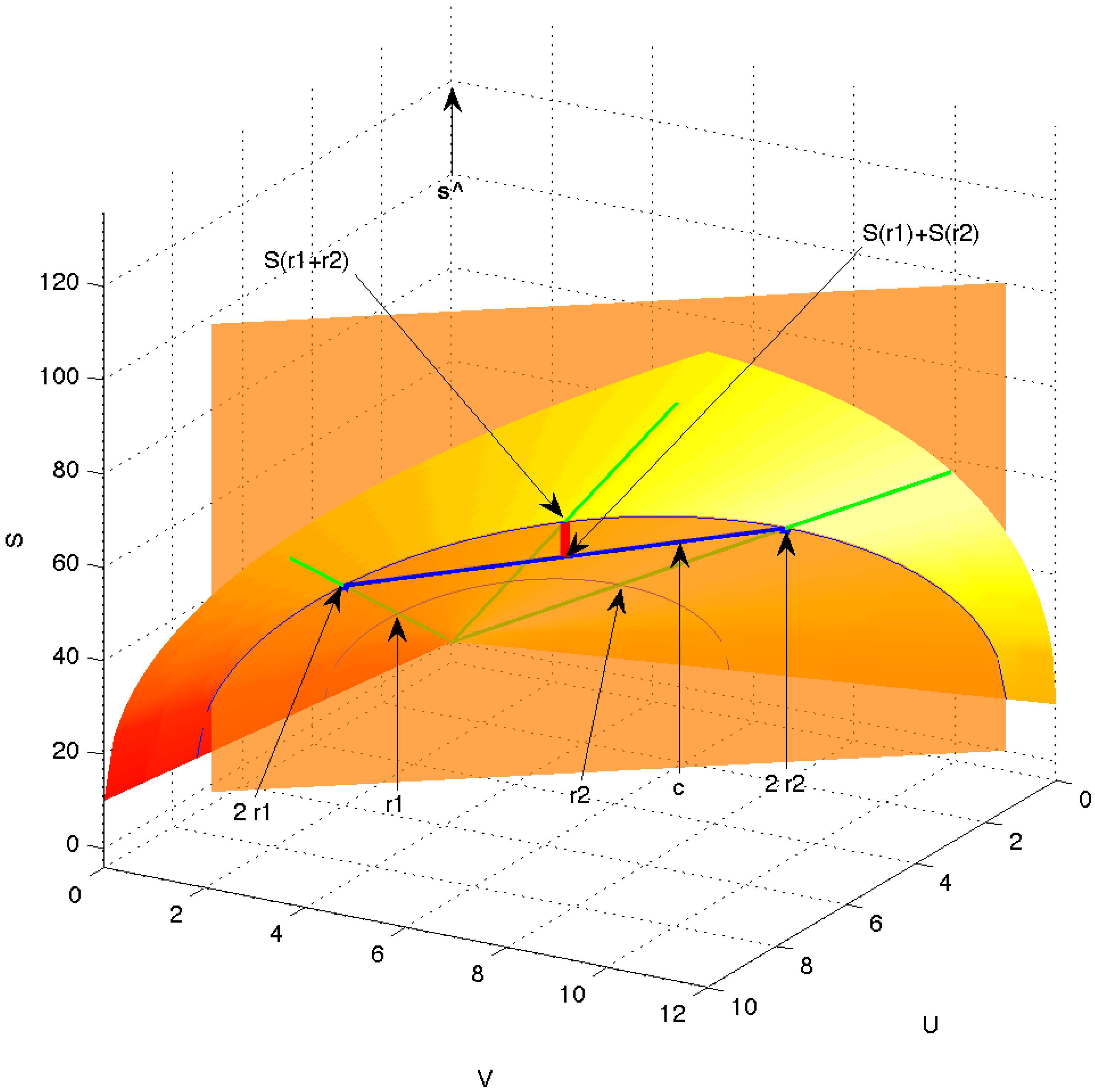
for homogeneous systems (thus disregarding surface, interface, and all long range interaction effects here), $\lambda \mathbf{r}$ is just a scaled version of the same thermodynamic state. Thus, changes of state along radial lines from the origin are degenerate in that no internal thermodynamic process is required to move between them. They only correspond to different amounts of the same equilibrium system. This is a global requirement on all thermodynamic systems. This scaling is illustrated in Figure 6, where the shaded bandshell-like surface is the equilibrium surface within the three-dimensional space of $\{S,U,V\}$. The green rays emanating from the origin represent equivalent equilibrium states, differing only in magnitude, e.g., states ${\mathbf{r}}_1$ and ${2\mathbf{r}}_1$.

Figure 6. Equilibrium surface $S(U,V)$ (shaded bandshell-like surface) in the space of extensive variables $\{S,U,V\}$. The green rays emanating from the origin represent equivalent equilibrium states, differing only in magnitude, e.g., states ${\mathbf{r}}_1$ and $2{\mathbf{r}}_1$. The vector $\mathbf{c}$ (thick blue line) is a chord connecting the two equilibrium points $2{\mathbf{r}}_1$ and $2{\mathbf{r}}_2$ on the equilibrium surface but otherwise being under the surface and thus passing through non-equilibrium states. The equilibrated mixture of ${\mathbf{r}}_1$ and ${\mathbf{r}}_2$ is indicated as $S({\mathbf{r}}_1+{\mathbf{r}}_2)$ and the entropy produced in the equilibration is shown as the short, thick red line.

Figure 6. Equilibrium surface $S(U,V)$ (shaded bandshell-like surface) in the space of extensive variables $\{S,U,V\}$. The green rays emanating from the origin represent equivalent equilibrium states, differing only in magnitude, e.g., states ${\mathbf{r}}_1$ and $2{\mathbf{r}}_1$. The vector $\mathbf{c}$ (thick blue line) is a chord connecting the two equilibrium points $2{\mathbf{r}}_1$ and $2{\mathbf{r}}_2$ on the equilibrium surface but otherwise being under the surface and thus passing through non-equilibrium states. The equilibrated mixture of ${\mathbf{r}}_1$ and ${\mathbf{r}}_2$ is indicated as $S({\mathbf{r}}_1+{\mathbf{r}}_2)$ and the entropy produced in the equilibration is shown as the short, thick red line.

On the other hand, joining two independent systems denoted by their state vectors ${\mathbf{r}}_1$ and ${\mathbf{r}}_2$ that do not follow on the same radial line is a different matter. Pure additivity would yield a state ${\mathbf{r}}_1+{\mathbf{r}}_2$. That is, the resulting entropy would be given (incorrectly) by

$$S\left({\mathbf{r}}_1\right)+S\left({\mathbf{r}}_2\right)=S({\mathbf{r}}_1+{\mathbf{r}}_2)$$

(17)

based on pure extensivity, if state functions did not have to reflect the second law. But the second law of thermodynamics requires that not all extensities can be additive after an irreversible interaction between systems defined by ${\mathbf{r}}_1$ and ${\mathbf{r}}_2$. In particular, if $U,V,n_1,n_2,\cdots$ remain additive (i.e., their total amounts remain fixed before and after the systems are joined), then the total entropy must increase,

$$S\left({\mathbf{r}}_1\right)+S\left({\mathbf{r}}_2\right)\le S({\mathbf{r}}_1+{\mathbf{r}}_2).$$

(18)

Here, it is important to remember that the space depicted in Figure 6 represents possible extensities of a system, equilibrium as well as non-equilibrium.

The vector $\mathbf{c}=2{\mathbf{r}}_2-2{\mathbf{r}}_1$, joining $2{\mathbf{r}}_1$ to $2{\mathbf{r}}_2$ (marked in blue in Figure 6), and the unit vector along the S-axis, $\widehat{\mathbf{s}}$, together define a plane. This is the vertical plane in Figure 6, which is drawn semitransparent in order to allow view of the origin, the original equilibrium states ${\mathbf{r}}_1$ and ${\mathbf{r}}_2$, and the full green scaling rays. In that plane, the irreversibility indicated by the inequality Equation (18), i.e., the difference between the equilibrated entropy $S({\mathbf{r}}_1+{\mathbf{r}}_2)$ and the unequilibrated, merely scaled entropy $S\left({\mathbf{r}}_1\right)+S\left({\mathbf{r}}_2\right)$, is shown by the thick red line.

Since the states represented by ${\mathbf{r}}_1$ and ${\mathbf{r}}_2$ are arbitrary, Equation (18) reduces to the standard definition of a convex function in the plane defined by $\mathbf{c}$ and $\widehat{\mathbf{s}}$. As long as ${\mathbf{r}}_1$ and ${\mathbf{r}}_2$ are not parallel, this reasoning is true for any such plane, thus requiring the surface itself be convex. The second law of thermodynamics consequently necessitates the convexity of the principal equation of state function in the entropy picture, $S(U,V,n_1,n_2,\cdots )$ and equivalently the convexity of the principal equation of state function in the energy picture, $U(S,V,n_1,n_2,\cdots )$. Thus, the second law of thermodynamics shows up in the convexity of the equilibrium surface. Not only is this conceptually important, the principal equation of state guarantees agreement with the second law for all processes.

We now return to the energy picture and observe that the eigenvalues of the Hessian are the practical indicator for convexity. At some $\mathbf{r}$ we may define a parameter t along a direction represented by the vector $\mathbf{h}=\left(h_1,h_2,\cdots ,h_n\right)$. Then

$$U\left(t\right)=U\left(0\right)+{\left.\frac{dU}{dt}\right|}_{t=0}t+{\left.\frac{1}{2}\frac{d^{2}U}{d{t}^2}\right|}_{t=0}{t}^2+O\left(t^3\right).$$

(19)

The second term is the derivative along $\mathbf{h}$ with respect to t, while the third is the second directional derivative. Along $\mathbf{h}$

$$U(\mathbf{r}+t\mathbf{h})=U\left(\mathbf{r}\right)+\sum _{i=1}^n{U}_{h_i}\left(\mathbf{r}\right)h_{i}t+\frac{1}{2}\sum _{j=1}^n\sum _{i=1}^n{U}_{h_i{h}_j}\left(\mathbf{r}\right)h_i{h}_j{t}^2+O\left(t^3\right).$$

(20)

Here, we have used the notation $U_x=\partial U/\partial x$. The double sum is the second directional derivative, which can be rewritten as

$$\sum _{j=1}^n\sum _{i=1}^n{U}_{h_i{h}_j}\left(\mathbf{r}\right)h_i{h}_j={\mathbf{h}}^T\mathcal{H}\left(\mathbf{r}\right)\mathbf{h},$$

(21)

just in a more general mathematical nomenclature. Here $\mathcal{H}$ is the matrix of second derivatives, $U_{ij}$, known as the Hessian. This is the same as Weinhold’s metric Equation (1). As the right side is a quadratic form in $\mathbf{h}$, the sign of the second derivative or curvature for any direction $\mathbf{h}$ is determined by the eigenvalues of $\mathcal{H}$. In particular, convexity guarantees for the case of the energy representation $U(S,V,n_1,n_2,\cdots )$ that the eigenvalues will all be positive, except when $\mathbf{h}$ is a direction that implies a position vector $\mathbf{r}$ on the equilibrium surface. In that case the eigenvalue must be 0, because scaling requires that the surface be flat in that direction. This situation was already mentioned in Section 2. Therefore, all Hessians of principal equations of state will certainly have one zero eigenvalue and it follows that their determinants will always vanish. Moreover, because they are symmetric, all eigenvectors other than $\mathbf{r}$ will be orthogonal to the position vector $\mathbf{r}$. Further details may be found in [12].

7. Conclusions

In its 40 years of existence, Weinhold’s thermodynamic metric has proven its tremendous usefulness in providing lower bounds for dissipation in just about any process, be it in thermodynamics, economics, or other disciplines. We have described the underlying equations of state and the restrictions put on those by the second law of thermodynamics, and we have presented examples of heat converting processes, chemical reactions, and from economics. Even general optimization methods like simulated annealing have taken over elements from the metric bound Equation (3), in that the optimal path is the one which proceeds at constant thermodynamic speed [32,33].

Geometric formulations of mechanics, relativity, cosmology, quantum mechanics, high energy physics etc. have proven exceptionally useful, not least in providing a framework for describing the processes being investigated. Another important contribution is in limiting what is possible. It was about time that this tool entered thermodynamics and also statistical mechanics. Considering the impact it has already had, much more promises to be in store.