A Gloss Composition and Context Clustering Based Distributed Word Sense Representation Model

Abstract

In recent years, there has been an increasing interest in learning a distributed representation of word sense. Traditional context clustering based models usually require careful tuning of model parameters, and typically perform worse on infrequent word senses. This paper presents a novel approach which addresses these limitations by first initializing the word sense embeddings through learning sentence-level embeddings from WordNet glosses using a convolutional neural networks. The initialized word sense embeddings are used by a context clustering based model to generate the distributed representations of word senses. Our learned representations outperform the publicly available embeddings on half of the metrics in the word similarity task, 6 out of 13 sub tasks in the analogical reasoning task, and gives the best overall accuracy in the word sense effect classification task, which shows the effectiveness of our proposed distributed distribution learning model.

1. Introduction

The representation of knowledge has become focal areas in natural language processing. There have been many different methods for conceptual information representation. These range from extreme localist theories in which each concept is represented by a single unit (symbolic or distributional representation) to extreme distributed theories in which a concept corresponds to a pattern of activity over a large part of the cortex (distributed representation) [1].

With the rapid development of deep neural networks and parallel computing, distributed representation of knowledge attracts much research interest. Models for learning distributed representations of knowledge have been proposed at different granularity levels, including word sense level [2,3,4,5,6], word level [7,8,9,10,11,12], phrase level [13,14,15], sentence level [11,16,17,18,19], discourse level [20] and document level [19].

Distributed representation of word senses refers to represent word senses in a low-dimensional space for conveying the semantic information contained in the words. Usually, a word sense is represented as a dense and real-valued vector. To this end, most existing approaches adopted a cluster-based paradigm, which produces different sense vectors for each polysemy or homonymy through clustering the context of the target words. However, this paradigm usually has two limitations: (1) The performance of these approaches is sensitive to the clustering algorithm which requires the setting of the sense number for each word. For example, Neelakantan et al. [4] proposed two clustering based model: the Multi-Sense Skip-Gram (MSSG) model and Non-Parametric Multi-Sense Skip-Gram (NP-MSSG) model. MSSG assumes each word has the same k-sense (e.g., k = 3), i.e., the same number of possible senses. However, the number of senses in WordNet [21] varies from 1 such as “ben” to 75 such as “break”. As such, fixing the number of senses for all words would result in poor representations. NP-MSSG requires a tuning of a hyperparameter λ which controls the creation of cluster centroids during training. Different λs need to be tuned for different datasets; (2) The initial value of sense representation is critical for most statistical clustering based approaches. However, previous approaches usually adopted random initialization [4] or mean average of the candidates words in a gloss [3]. As a result, they may not produce optimal clustering results for word senses.

Focusing on the aforementioned two problems, this paper proposes to learn distributed representations of word senses through WordNet gloss composition and context clustering. The basic idea is that a word sense is represented as a synonym set (synset) in WordNet. In this way, instead of assigning a fixed sense number to each word as in the previous methods, different words will be assigned with different number of senses based on their corresponding entries in WordNet. Moreover, we notice that each synset has a textual definition (named gloss). Naturally, we use a convolutional neural network (CNN) to learn distributed representations of these glosses (a.k.a. sense vectors) through sentence composition. Then, we modify the MSSG algorithm for context clustering by initializing the sense vectors with the representations learned by our CNN-based sentence composition model. We expect that word sense vectors initialized in this way would lead to more precise representations of word senses generated from context clustering.

The obtained word sense representations are evaluated on three tasks: a word similarity task on two datasets, an analogical reasoning task provided by WordRep [22], and word sense effect classification task. The results show that our approach attains comparable performance on learning distributed representations of word senses. In specific, our learned representation outperforms publicly available embeddings on half of the metrics in word similarity task, and 6 in 13 subtasks in the analogical reasoning task. In the sense effect classification task, we achieve the state-of-the-art results. The results show that our approach attains an overall better performance on learning distributed representations of word senses.

The main contributions of this work are as follows: (1) we propose to use a sentence composition model to capture word sense from a knowledge base, e.g., WordNet; (2) while previous approaches to sense vector clustering often adopted random initialization, we propose to initialize sense vectors and the number of sense clusters with the word sense knowledge learned from WordNet for better clustering results; (3) we further verify our learned distributed word sense representations on three different tasks, word similarity measurement, analogical reasoning and word sense effect classification. Our approach achieves comparable results compared to the existing distributed word sense representation learning models on the first two tasks and gives the state-of-the-art results on the last task.

The rest of this paper is organized as follows. Section 2 reviews related work. Section 3 presents our proposed model. Section 4 describes the evaluation results and presents discussions. Section 5 concludes the paper and outlines future research directions.

2. Related Work

2.1. Distributed Representation for Word Sense

Most distributed word sense representation approaches are derived from distributed single prototype word representation approach first proposed by Rummelhart [7] and then have become a successful paradigm, especially for neural probabilistic language models [8,9,10,11,12].

Reisinger and Mooney [23] proposed a multi-prototype vector space model using the context cluster of each word to generate a distinct prototype vector for a word. Huang et al. [2] followed this idea, but introduced a probabilistic neural language model to generate distributed representations instead of distributional representations. Their approach first represents each word by a vector averaged over its context window comprising of five words before, five words after and the word itself. The spherical k-means algorithm is then used to cluster such context representations. Each word occurred in the corpus is re-labeled by its associated cluster and is used to train the distributed representation for that cluster.

Tian et al. [5] integrated a probabilistic multi-prototype model into the continuous skip-gram model. Expectation Maximization (EM) algorithm is used to learn multiple embeddings for polysemy. Motivated by the intuition that the same word in a source language with different senses is supposed to have different translations in a foreign language, Guo et al. [6] proposed a distributed word senses representation approach by clustering translated words from bilingual parallel data. Neelakantan et al. [4] presented an extension to the skip-gram model to learn word sense representation by non-parametrically estimating the number of senses per word type. Chen et al. [3] used glosses in WordNet as clues for learning distributed representation of word sense. But they simply represent each word sense by the vector averaged over all the words occurred in the corresponding gloss which may not be able to produce a good word sense representation.

2.2. Distributed Sentence Composition Model

Distributed Sentence Composition refers to representing a sentence in a low-dimensional space for conveying the semantic information contained in the sentence. Various types of distributed sentence representation models have been proposed recently. Socher et al. [16] proposed a recursive neural tensor network (RNTN) for semantic compositionality over a sentiment Treebank which pushes the binary classification accuracy on Stanford sentiment tree bank from 80% up to 85.4%. Kalchbrenner et al. [17] proposed a dynamic convolutional neural network (DCNN) to handles the input sentences with varying length and induced a feature graph over the sentence that is capable of explicitly capturing short and long-range relations. It improves the above accuracy from 85.4% to 86.8%. Kim [18] presented two simple CNN models with little hyper parameter tuning which are trained on pre-trained word vectors for sentence-level classification tasks. It further improves the above accuracy to 88.1%. Le and Mikolov [19] proposed an unsupervised algorithm that learns fixed-length feature representations from variable-length pieces of texts, such as sentences, paragraphs and documents. The recurrent neural network (RNN) may also be viewed as a sentence model. The layer computed at the last word represents the sentence [11,17].

3. Our Approach

In this study, we propose to learn distributed representation of word sense learning approach by incorporating WordNet gloss compositionality and context words clustering in large-scale raw text. The system framework with three main components is shown in Figure 1. The first component, the Word Embedding Construction Module, takes a large collection of raw text to train a word embedding model. The word embeddings output by the model are then used by a Sentence Composition Model, which takes glosses in WordNet as positive training data and randomly replacing part of the words as negative training data to construct the corresponding word sense vectors based on the one-dimensional CNN. The learned sense vectors are fed into a variant of the previously proposed Multi-Sense Skip-Gram Model (MSSG) to generates distributed representations of word senses from a text corpus. We name our approach as CNN-VMSSG.

Figure 1. Framework of our approach.

Figure 1. Framework of our approach.

3.1. Word Embedding Construction

Mikolov et al. [12] introduced the Continuous Bag-Of-Words (CBOW) model and continuous skip-gram model (Skip-gram) to learn vector representations for capturing a large number of syntactic and semantic word relationships from unstructured text data. The training objective of CBOW model is to use the surrounding words of a target word in a sentence or a document to predictits representation representation. Given a sequence of training words w₁, w₂, w₃ … w_T, the training objective is to maximize the average log probability:

$$\frac{1}{T}{\displaystyle \sum _{t=1}^T}{\displaystyle \sum _{-c\le i\le c,i\ne 0}}logp\left(w_t\right|w_{t+i})$$

(1)

where c is the size of the training context, w_t is the center word, and $logp\left(w_t\right|w_{t+i})$ is the conditional log probability of the center word w_t given the surrounding words w_t+i. The prediction task is performed via softmax. The hierarchical softmax [10,24] process which uses a binary tree representation of the output layer with the words as leaves, is used to reduce computational complexity.

3.2. Training Sense Vectors from WordNet Glosses Using CNN

Most of the glosses in WordNet are single sentence. We learn the distributed representation of each gloss sentence as the representation of the corresponding synset.

3.2.1. Training Objective

The training objective of this component is similar to the training objective proposed in [2,9] where the goal is to maximize the conditionalprobability of observing the actual target word given the input context. A common practice is to replace each target word by a random word to create negative training examples. Our goal is to model glosses in WordNet. Here, we replace several words in the gloss sentence to construct a negative sample at a time.

Given a gloss sentence s as a positive training sample, we randomly replace some words (controlled by a parameter λ) in s to construct a negative training sample s′. We compute scores f(s) and f(s′) where f(·) is the scoring function represents the whole CNN architecture without the softmax layer. We expect f(s) to be approximating 1, f(s′) to be approximating 0, and f(s) to be larger than f(s′) by a margin of 1 for all the sentences in the positive training set P. So the training objective is to minimize the ranking loss below:

$$G_s={\displaystyle \sum _{s\in P}}max\{0,1-f\left(s\right)+f\left(s^{\prime }\right)\}$$

(2)

3.2.2. Neural Network Architecture

The CNN architecture, shown in Figure 2 is used to model the glosses in WordNet. It follows the architecture proposed by [18] (The source code provided by the authors of this paper is available at https://github.com/yoonkim/CNN_sentence) which is a slight variant of the architecture proposed by [9]. It takes a gloss matrix s as input where each column corresponds to the distributed representation $v_{w_i}\in {\mathbb{R}}^d$ of a word w_i in the sentence or a padding vector $v_{z_i}\in {\mathbb{R}}^d$:

$$s=[v_{z_1},\cdots ,v_{z_{m-1}},v_{w_1},\cdots ,v_{w_n},v_{z_1},\cdots ,v_{z_{m-1}}]$$

(3)

where $v_{w_i}$ is a d dimensional pre-trained word vector constructed from a large corpus by CBOW model, $v_{z_i}$ is a d dimensional zero vector, m is the size of a filter window, n is defined as the maximum length of sentences in the training set. There are two types of convolution operation: the narrow one and the wide one [17]. We use the wide type in this paper in which the padding vectors $v_{z_1}$ to $v_{z_{m-1}}$ at the beginning and the end of the sentence are used to make sure the convolution operation can be done from the beginning of the sentence until the end of the sentence.

Figure 2. A one-dimensional convolutional neural network (CNN) with two filter widths for an example gloss sentence.

Figure 2. A one-dimensional convolutional neural network (CNN) with two filter widths for an example gloss sentence.

The idea behind the one-dimensional convolution is to take the dot product of the vector w with each m-gram in the sentence s to obtain another sequence c. In the convolutional layer, one-dimensional convolution is taken between a filter vector $w\in {\mathbb{R}}^{md}$ and a vector $s_{i:i+m-1}\in {\mathbb{R}}^{md}$ of m concatenated columns in s. The i-th feature $c_i\in \mathbb{R}$ of a feature map $F_j\in {\mathbb{R}}^{n+m-1}$ is generated as follows:

$$c_i=f(w·s_{i:i+m-1}+b)$$

(4)

where b ∈ ℝ is a bias term and f is a point-wise non-linear function such as the hyperbolic tangent. $s_{i:i+m-1}$ refers to columns from i to i + m − 1 of s. In order to make c cover different words in the negative sample corresponding a positive sample, in this work, we randomly replace half of the words in a positive training sample to construct a negative training sample (λ = 0.5). A feature map $F_j\in {\mathbb{R}}^{n+m-1}$ is defined as

$$F_j=[c_1,c_2,\cdots ,c_{n+m-1}]$$

(5)

In the pooling layer, a max-overtime pooling operation [25], which forces the network to capture the most useful local features produced by the convolutional layers, is applied over F_j. The maximum value $\widehat{F_j}=max\left(F_j\right)$ is the feature corresponding to a particular filter w. The $\widehat{F_j}$ of k filters are concatenated to form a vector $\widehat{F}\in {\mathbb{R}}^k$. The model uses multiple filters (with varying window sizes) to obtain multiple features. These features form the penultimate layer and are passed to a fully connected softmax layer whose output is the probability distribution over labels. The training error propagates back to fine-tune the parameters (w, b) and the input word vectors. The vector generated in the penultimate layer of the CNN architecture is regarded as the sense vector which captures the semantic content of the input gloss, to some degree.

3.3. Context Clustering and VMSSG Model

The sense vectors trained from WordNet glosses using CNN doesn’t perform well on some word sense evaluation tasks, partly because the semantic meaning of the actual context that a word occurs may not be similar to the gloss of the synset in which the word belongs to. To deal with this problem, we propose to incorporate the sense vectors learned from WordNet glosses by CNN composition as prior knowledge into a context clustering model such as the MSSG model proposed by Neelakantan et al. [4]

The MSSG model extends the skip-gram model to learn multi-prototype word embeddings by clustering the word embeddings of context words around each word. In this model, for each word w, the corresponding word embedding $v_w\in {\mathbb{R}}^d$, k-sense vector $v_{s_k}\in {\mathbb{R}}^d$ (k = 1, 2,…, K) and k-context cluster with center ${\mu }_k\in {\mathbb{R}}^d$ (k = 1, 2,…, K) are initialized randomly. The sense number K of each word is a fixed parameter in the training algorithm.

Algorithm 1 Algorithm of VMSSG model.
1:	Input: D, d,$K_1,\dots ,K_w,\dots ,K_{\left|V\right|}, M$.
2:	Initialize: $\forall w\in V,k\in \{1,\dots ,K_w\}$, initialize $v_w$ to a pre-trained word vector, $v_{s_k^w}$ to a pre-trained sense vector for word w with sense k, and ${\mu }_k^w$ to a vector of random real value $\in {(-1,1)}^d$.
3:	for each w in D do
4:	r ← random number ∈ [1, M]
5:	C ← $\{w_{i-r},\dots ,w_{i-1},w_{i+1},\dots ,w_{i+r}\}$
6:	vc ← $\frac{1}{2\times r}{\sum }_{w\in C}{v}_w$
7:	$\widehat{k}$ = arg maxk {sim$({\mu }_k^w,v_c)$}
8:	Assign C to context cluster $\widehat{k}$
9:	Update ${\mu }_{\widehat{k}}$.
10:	C′ = NoisySamples (C)
11:	Gradient update on $v_{s_k^w}$, $v_w$ in $C,C^{\prime }$.
12:	end for
13:	Output: $v_{s_k^w}$, $v_w$, $\forall w\in V,k\in \{1,\dots ,K_w\}$

We improve the MSSG model in two different ways. Firstly, instead of setting a fixed number of senses K for each word as in the original MSSG, we set the sense number of each word based on its actual number of senses in the WordNet. By doing so, semantically rich words would have a larger number of senses and K becomes deterministic. Secondly, instead of randomly initializing sense vectors in the MSSG algorithm, we initialize sense vectors using those trained from WordNet glosses with CNN composition. In addition, we use the learned CBOW word embedding to initialize global word vectors v_w. We named this model as a variant of the MSSG (VMSSG) model.

The training algorithm of the VMSSG model is shown as Algorithm 1, where D is a text corpus, V is the vocabulary of D, |V| is the vocabulary size, M is the size of context window, v_w is the word embedding for w, $s_k^w$ is a kth context cluster of word w, ${\mu }_k^w$ is the centroid of cluster k for word w. The function NoisySamples(C) randomly replaces context words with noisy words from V.

4. Experiments

In this section, we first give a qualitative analysis by comparing the nearest neighbors of our embeddings with other embeddings. Next, we evaluate the performance of our word sense representations on three tasks, namely, word similarity task, analogical reasoning task, and word sense effect classification task respectively.

4.1. Experimental Setup

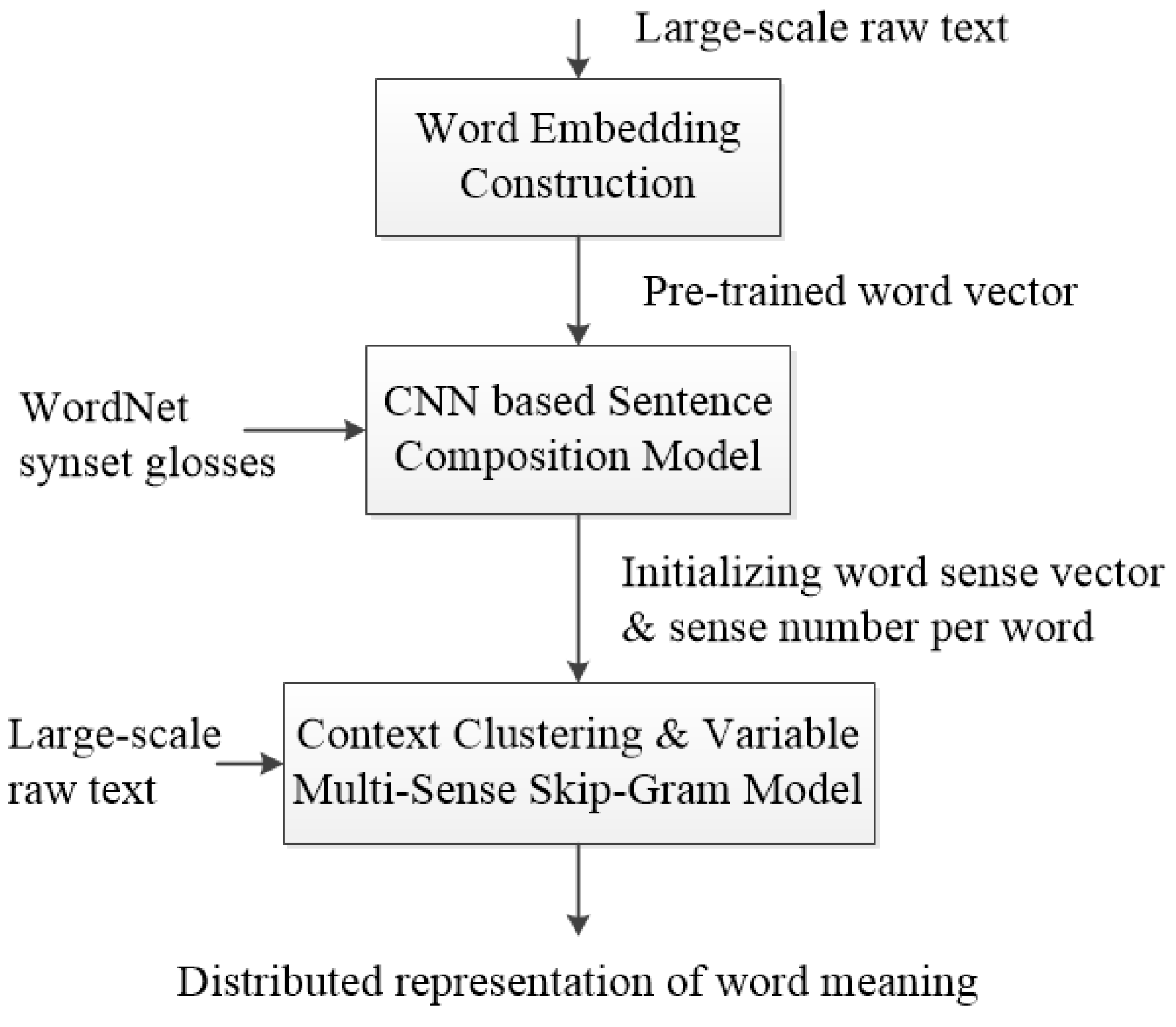
In all experiments, we use the publicly available word vectors trained on 100 billion words from Google News. The vectors have dimensionality of 300. They were trained using the CBOW model. For training sense vectors with VMSSG model, we use a snapshot of Wikipedia in April 2010 [26] previously used in [2,4]. WordNet 3.1 is used for training the sentence composition model.

For training CNN, we use: rectified linear units, filter windows of 3, 4, 5 with 100 feature maps each, AdaDelta decay parameter of 0.95, the dropout rate of 0.5. For training VMSSG, we use MSSG-KMeans as the clustering algorithm, and CBOW for learning sense vectors. We set the size of word vectors to 300, using boot vectors and sense vectors. For other parameter, we use default parameter settings for MSSG.

4.2. Qualitative Evaluations

In Table 1, Table 2 and Table 3, we list the nearest neighbors of each sense of three example words generated from two single-prototype word vector models (C & W and Skip-gram) and five multi-prototype word representation models. C & W refers to the word embedding published in [9]. Skip-gram refers to the language model proposed in [12]. Huang et al. refers to the multi-prototype word embedding proposed in [2]. Unified-WSR refers to the word sense embedding proposed in [3]. Both MSSG and NP-MSSG were previously proposed in [4] where MSSG assumes each word has the same number of senses and NP-MSSG extends from MSSG by automatically inferring the number of senses from data. CNN-VMSSG is our model. The column heading N of the tables shows the number of sense vectors generated by different models, and it is 1 for single-prototype word vector models. The nearest neighbor is selected by comparing the cosine similarity between each sense vector and all the sense vectors of other words in the vocabulary.

It is observed that single-prototype word vector models such as C & W and Skip-gram are not able to learn different sense representations for each word while Huang et al. and MSSG always generate a fixed number of sense vectors. NP-MSSG finds fewer number of sense vectors than the actual number of word senses. Our model can find a diverse range of word senses, for example, “edge” and “IMF” for bank, “MVP” and “circle” for star, “seed” and “Spedding” for plant. It shows that our model learns more different sense representations.

Table 1. Nearest neighbors of each sense of word bank.

Model	N	Nearest Neighbors
C & W	1	district
Skip-gram	1	banks
Huang et al.	10	memorabilia harbour cash corporation illegal branch distributed central corporation perth
Unified-WSR	18	banking_concern incline blood_bank bank_buildingn panoply piggy_bank ridge pecuniary_resource camber vertical_bank tip border transact agent turn_a_trick deposit steel trust
MSSG	3	banks savings river
NP-MSSG	2	banks banking
CNN-VMSSG	18	HDFC mouth credit Barclays almshouses banking bancshares subsidiary check joint edge Bancshares IMF strip reserve right frank depositors

Table 1. Nearest neighbors of each sense of word bank.

Model	N	Nearest Neighbors
C & W	1	district
Skip-gram	1	banks
Huang et al.	10	memorabilia harbour cash corporation illegal branch distributed central corporation perth
Unified-WSR	18	banking_concern incline blood_bank bank_buildingn panoply piggy_bank ridge pecuniary_resource camber vertical_bank tip border transact agent turn_a_trick deposit steel trust
MSSG	3	banks savings river
NP-MSSG	2	banks banking
CNN-VMSSG	18	HDFC mouth credit Barclays almshouses banking bancshares subsidiary check joint edge Bancshares IMF strip reserve right frank depositors

Table 2. Nearest neighbors of each sense of word star.

Model	N	Nearest Neighbors
C & W	1	fist
Skip-gram	1	stars
Huang et al.	10	princess silver energy version workshop guard appearance fictional die galaxy
Unified-WSR	12	supergiant ace starlet hexagram headliner asterisk star_topology co-star lead premiere dot leading
MSSG	3	stars trek superstar
NP-MSSG	2	wars stars supergiant
CNN-VMSSG	12	cast galaxies Carradine MVP newspaper Ursae sign beat trek purple circle sun

Table 2. Nearest neighbors of each sense of word star.

Model	N	Nearest Neighbors
C & W	1	fist
Skip-gram	1	stars
Huang et al.	10	princess silver energy version workshop guard appearance fictional die galaxy
Unified-WSR	12	supergiant ace starlet hexagram headliner asterisk star_topology co-star lead premiere dot leading
MSSG	3	stars trek superstar
NP-MSSG	2	wars stars supergiant
CNN-VMSSG	12	cast galaxies Carradine MVP newspaper Ursae sign beat trek purple circle sun

Table 3. Nearest neighbors of each sense of word plant.

Model	N	Nearest Neighbors
C & W	1	yeast
Skip-gram	1	plants
Huang et al.	10	insect robust food seafood facility treatment facility natural matter vine
Unified-WSR	10	industrial_plant plant_life dodge tableau set engraft found restock bucket implant
MSSG	3	plants factory flowering
NP-MSSG	4	stars Fabaceae manufacturing power
CNN-VMSSG	10	mill power GWh production seed factory microbial Asteraceae tree Spedding

Table 3. Nearest neighbors of each sense of word plant.

Model	N	Nearest Neighbors
C & W	1	yeast
Skip-gram	1	plants
Huang et al.	10	insect robust food seafood facility treatment facility natural matter vine
Unified-WSR	10	industrial_plant plant_life dodge tableau set engraft found restock bucket implant
MSSG	3	plants factory flowering
NP-MSSG	4	stars Fabaceae manufacturing power
CNN-VMSSG	10	mill power GWh production seed factory microbial Asteraceae tree Spedding

4.3. Word Similarity Task

In this task, we evaluate our learned word sense embedding on two datasets: the WordSim-353 (WS353) dataset [27] and the Contextual Word Similarities (SCWS) dataset [2], respectively.

WS353 dataset consists of 353 pairs of nouns. Each pair is associated with 13 to 16 human judgments on similarity and relatedness on a scale from 0 to 10. For example, (car, flight) received an average score of 4.94, while (car, automobile) received an average score of 8.94.

SCWS dataset contains 2003 pairs of words and their sentential contexts. It consists of 1328 noun-noun pairs, 399 verb-verb, 140 verb-noun, 97 adjective-adjective, 30 noun-adjective, and 9 verb-adjective. 241 pairs are same-word pairs. Each pair is associated with 10 human judgments of similarity on a scale from 0 to 10.

We use the same metrics in [4] to measure the similarity between two words w and w′ given their respective context c and c′. The avgSim metric computes the average similarity of all pairs of prototype vectors for each word, ignoring information from the context:

$$\text{avgSim}(w,w^{\prime })=\frac{1}{K_1{K}_2}{\displaystyle \sum _{i=1}^{K_1}}{\displaystyle \sum _{j=1}^{K_2}}d\left(v_{s_i}\left(w\right),v_{s_j}\left(w^{\prime }\right)\right)$$

(6)

where d(·, ·) is a standard distributional similarity measure. Here, cosine similarity is adopted. $v_{s_i}\left(w\right)$ is the sense vector of w. K₁, K₂ are the numbers of word senses of w and w′, respectively. The avgSimC metric weights each similarity term in avgSim by the likelihood of the word context appearing in its respective cluster:

$$\begin{array}{cc}\hfill \text{avgSimC}(w,w^{\prime })=\frac{1}{K_1{K}_2}\sum _{i=1}^{K_1}\sum _{j=1}^{K_2}& d_{c,w,i}{d}_{c^{\prime },w^{\prime },j}d\left(v_{s_i}\left(w\right),v_{s_j}\left(w^{\prime }\right)\right)\hfill \end{array}$$

where $d_{c,w,i}=d\left(v_c,{\pi }_i\left(w\right)\right)$ is the likelihood of context c belonging to cluster ${\pi }_i\left(w\right)$. The globalSim metric computes each word vector ignoring the many senses:

$$\text{globalSim}(w,w^{\prime })=d\left(v_w,v_{w^{\prime }}\right)$$

(7)

The localSim metric chooses the most similar sense in context to estimate the similarity of word pairs:

$$\text{localSim}(w,w^{\prime })=d\left(v_{s_k}\left(w\right),v_{s_{k^{\prime }}}\left(w^{\prime }\right)\right)$$

(8)

where $k={arg\; max}_i{d}_{c,w,i}$ and $k^{\prime }={arg\; max}_j{d}_{c^{\prime },w^{\prime },j}$.

We report the Spearman’s correlation ρ × 100 between a model’s similarity scores and the human judgements in the datasets.

Table 4 shows the performance achieved on the WordSim-353 dataset. In this table, the avgSimC and localSim metrics are not given since no context is provided in this dataset. Random-VMSSG refers to MSSG trained with the sense number of each word taken from WordNet. Average-VMSSG refers to MSSG trained with the average vector of the candidate word vectors of WordNet glosses which has previously proposed by Chen et al. [3]. In Average-VMSSG, for each sense sense_i of word w, a candidate set from golss(sense_i) is defined as follows:

$$\text{cand}\left(sens{e}_i\right)=\left\{u\right|u\in \text{gloss}\left(sens{e}_i\right),u\ne w,\text{POS}\left(u\right)\in CW,\text{cos}(v_w,v_u))>\sigma \}$$

(9)

where POS(u) is the part-of-speech tagging of the word u and CW is the set of possible part-of speech tags in WordNet: noun, verb, adjective and adverb. v_w and v_u are word vectors of w and u, respectively. Following Chen et al. [3], we set the similarity threshold σ = 0 in this experiment. The average of the word vectors in cand(sense_i) is used to initialize sense vectors in the VMSSG model.

Table 4. Experimental results in the WordSim-353 (WS353) task. We compute the avgSim value using the published word vectors for Unified-WSR 200 d. Other results of the compared models, e.g., Huang et al., Non-Parametric Multi-Sense Skip-Gram (NP-MSSG) and MSSG, were reported in [4]. 50 d, 200 d and 300 d refer to the dimension of the vector. The best results are highlighted in bold face.

Model	avgSim	globalSim
Huang et al. 50 d	64.2	22.8
Unified-WSR 200 d	41.4	-
NP-MSSG 300 d	68.6	69.1
MSSG 300 d	70.9	69.2
Random-VMSSG 300 d	63.3	69.1
Average-VMSSG 300 d	61.5	69.2
CNN-VMSSG 300 d	64.4	69.8
Pruned TF-IDF	73.4	-
ESA	-	75.0
Tiered TF-IDF	76.9	-

Table 4. Experimental results in the WordSim-353 (WS353) task. We compute the avgSim value using the published word vectors for Unified-WSR 200 d. Other results of the compared models, e.g., Huang et al., Non-Parametric Multi-Sense Skip-Gram (NP-MSSG) and MSSG, were reported in [4]. 50 d, 200 d and 300 d refer to the dimension of the vector. The best results are highlighted in bold face.

Model	avgSim	globalSim
Huang et al. 50 d	64.2	22.8
Unified-WSR 200 d	41.4	-
NP-MSSG 300 d	68.6	69.1
MSSG 300 d	70.9	69.2
Random-VMSSG 300 d	63.3	69.1
Average-VMSSG 300 d	61.5	69.2
CNN-VMSSG 300 d	64.4	69.8
Pruned TF-IDF	73.4	-
ESA	-	75.0
Tiered TF-IDF	76.9	-

We also present the results obtained using the word distributional representations including Pruned TF-IDF [23], Tiered TF-IDF [28] and Explicit Semantic Analysis (ESA) [29]. Pruned TF-IDF and Tiered TF-IDF combine the vector-space model and context clustering. TF-IDF represents words in a word-word matrix capturing co-occurrence counts in all context windows. Pruned TF-IDF prunes the low-value TF-IDF features while Tiered TF-IDF uses tiered clustering that leverages feature exchangeability to allocate data features between a clustering model and shared components. ESA explicitly represents the meaning of texts in a high-dimensional space of concepts derived from Wikipedia.

It is observed that our model achieves the best performance on the globalSim metric. It indicates that the use of pre-trained word vector and initializing word sense vector is helpful to improve the quality of global word vector generated by CNN-VMSSG. Unified-WSR has the same number of senses as in our model but gives a much worse result on avgSim, being 23.0% lower. Random-VMSSG also takes the same number of senses for each word from WordNet as in our model but still performs worse on both avgSim and globalSim. CNN-VMSSG is 2.9% higher than Average-VMSSG on the avgSim metric (64.4 vs. 61.5), and 0.6% higher than Average-VMSSG on the globalSim metric (69.8 vs. 69.2), respectively. It indicates that the WordNet glosses composition approach proposed in our model performs better than using the average of the candidate word vectors of WordNet glosses.

Our model gives lower avgSim results compared to MSSG and NP-MSSG. One possible reason is that we set the number of context clusters for each word to be the same as the number of its corresponding senses in WordNet. However, not all senses appear in the our experimented corpus which could lead to fragmented context clustering results. One possible way to alleviate this problem is to perform post-processing to merge clusters which have smaller inter-cluster differences or to remove sense clusters which are under-represented in our data. We will leave it as our future work.

We report the Spearman’s correlation ρ × 100 between a model’s similarity scores and the human judgements of SCWS dataset in Table 5. It is observed that our model achieves the best performance on the globalSim and localSim metrics, being 0.8% higher on globalSim and 1.3% higher on localSim compared to the second best performing model NP-MSSG. Comparing with Average-VMSSG, our model achieves better performance on all the four metrics. It indicates that the CNN composition approach proposed in our model is beneficial for this task. Our approach however performs worse on avgSim and avgSimC possibly due to the same reason explained for the WS353 task.

Table 5. Experimental results in the Contextual Word Similarities (SCWS) task. We compute the evaluation results using the published word vectors for Unified-WSR 200 d. Other results of the compared models, e.g., Huang et al., NP-MSSG and MSSG, were reported in [4].

Model	globalSim	avgSim	avgSimC	localSim
Huang et al. 50 d	58.6	62.8	65.7	26.1
Unified-WSR 200 d	64.2	66.2	68.9	-
NP-MSSG 300 d	65.5	67.3	69.1	59.8
MSSG 300 d	65.3	67.2	69.3	57.3
Random-VMSSG 300 d	65.4	65.3	65.7	58.1
Average-VMSSG 300 d	65.5	64.9	65.9	59.2
CNN-VMSSG 300 d	66.3	65.7	66.4	61.1

Table 5. Experimental results in the Contextual Word Similarities (SCWS) task. We compute the evaluation results using the published word vectors for Unified-WSR 200 d. Other results of the compared models, e.g., Huang et al., NP-MSSG and MSSG, were reported in [4].

Model	globalSim	avgSim	avgSimC	localSim
Huang et al. 50 d	58.6	62.8	65.7	26.1
Unified-WSR 200 d	64.2	66.2	68.9	-
NP-MSSG 300 d	65.5	67.3	69.1	59.8
MSSG 300 d	65.3	67.2	69.3	57.3
Random-VMSSG 300 d	65.4	65.3	65.7	58.1
Average-VMSSG 300 d	65.5	64.9	65.9	59.2
CNN-VMSSG 300 d	66.3	65.7	66.4	61.1

4.4. Analogical Reasoning Task

The analogical reasoning task introduced by [12] consists of questions of the form “a is to b as c is to _”, where (a, b) and (c, _) are two word pairs. The goal is to find a word d* in vocabulary V whose representation vector is the closest to $v_b-v_a+v_c$, i.e.,

$$d^{*}=\underset{w\in V,w\ne b,w\ne c}{arg\; min}sim\left((v_b-v_a+v_c),v_w\right)$$

(10)

The question is judged as correctly-answered only if d* is exactly the answer word in the evaluation set [22].

WordRep is a benchmark collection for research on learning distributed word representations, which expands the Mikolov et al.’s analogical reasoning questions. It includes two kinds of evaluation sets: an enlarged evaluation set where the word pairs are collected from Wikipedia, and WordNet evaluation set where the word pairs are collected from WordNet. Considering the size of evaluation set, in our experiments, we use one evaluation set in WordRep, the WordNet collection which consists of 13 sub tasks. Let the sense numbers of a, b, c be $N_a$, $N_b$, $N_c$, and the size of vocabulary be $V_{size}$, the number of candidate vectors for a word sense model is $N_a\times N_b\times N_c\times V_{size}$, while it is only $V_{size}$ for single-prototype word vector models. This shows that the evaluation task is computationally more complicated for the word sense based models than for the single prototype models.

Table 6 shows the precision results on the 13 sub tasks. The Word Pair column is the number of word pairs of each sub task ($N_{wp}$). The results of C&W were obtained using the 50-dimensional word embeddings that were made publicly available by Turian et al. [30]. The CBOW results were previously reported in [22]. Weighted Average is computed as follows:

$$\text{weightedAvg}=(N_{wp}^2÷2)\times p$$

(11)

It can be observed that our learned representations outperform all the other 4 embeddings on weighted average. Among 13 sub tasks, our model outperforms the others by a good margin in six sub tasks, Attribute, Causes, Entails, IsA, MadeOf and RelatedTo. Overall, our model gives superior performance compared to all the other models.

Table 6. Experimental results in the analogical reasoning task. The numbers are the precision p × 100.

Subtask	Word Pairs	C & W	CBOW	MSSG	NP-MSSG	CNN-VMSSG
Antonym	973	0.28	4.57	0.25	0.10	1.01
Attribute	184	0.22	1.18	0.03	0.15	1.63
Causes	26	0.00	1.08	0.31	0.31	1.23
DerivedFrom	6,119	0.05	0.63	0.09	0.05	0.17
Entails	114	0.05	0.38	0.49	0.34	1.29
HasContext	1,149	0.12	0.35	1.73	1.56	1.41
InstanceOf	1,314	0.08	0.58	2.52	2.34	2.46
IsA	10,615	0.07	0.67	0.15	0.08	0.86
MadeOf	63	0.03	0.72	0.80	0.48	1.28
MemberOf	406	0.08	1.06	0.14	0.86	0.90
PartOf	1,029	0.31	1.27	1.50	0.73	0.48
RelatedTo	102	0.00	0.05	0.12	0.11	1.28
SimilarTo	3,489	0.02	0.29	0.03	0.01	0.12
WeightedAvg		0.06	0.66	0.17	0.11	0.67

Table 6. Experimental results in the analogical reasoning task. The numbers are the precision p × 100.

Subtask	Word Pairs	C & W	CBOW	MSSG	NP-MSSG	CNN-VMSSG
Antonym	973	0.28	4.57	0.25	0.10	1.01
Attribute	184	0.22	1.18	0.03	0.15	1.63
Causes	26	0.00	1.08	0.31	0.31	1.23
DerivedFrom	6,119	0.05	0.63	0.09	0.05	0.17
Entails	114	0.05	0.38	0.49	0.34	1.29
HasContext	1,149	0.12	0.35	1.73	1.56	1.41
InstanceOf	1,314	0.08	0.58	2.52	2.34	2.46
IsA	10,615	0.07	0.67	0.15	0.08	0.86
MadeOf	63	0.03	0.72	0.80	0.48	1.28
MemberOf	406	0.08	1.06	0.14	0.86	0.90
PartOf	1,029	0.31	1.27	1.50	0.73	0.48
RelatedTo	102	0.00	0.05	0.12	0.11	1.28
SimilarTo	3,489	0.02	0.29	0.03	0.01	0.12
WeightedAvg		0.06	0.66	0.17	0.11	0.67

4.5. Word Sense Effect Classification

In this section, we evaluate our approach on word sense effect classification proposed by Choi and Wiebe [31]. In this task, each sense is annotated with three classes: + effect, − effect and Null. In total, 258 + effect senses, 487 − effect senses, and 440 Null senses are manually annotated as a word sense lexicon with the help of FrameNet [32]. Half of each set is used as training data, and the other half is used for evaluation.

Choi and Wiebe [31] propose three word sense effect classification methods, namely, supervised learning (onlySL) method, graph-based learning (onlyGraph) method and hybrid method. In the onlySL method, the gloss classifier (SVM) is trained with word features and sentiment features for WordNet Gloss. The method also uses WordNet relations and WordNet similarity information as training features. In the onlyGraph method, a graph is constructed by using WordNet relations, such as hypernymy, troponymy and grouping, and a graph-based semi-supervised learning method is used to perform label propagation. In the hybrid method, the results generated from onlySL and onlyGraph are combined by some rules, e.g., If the labels assigned by both models are + effect (or − effect), it is + effect (or − effect).

For evaluation metrics, we use precision (P × 100), recall (R × 100) and F1 score (F1 × 100) for each class, and an overall accuracy. For classifiers, we use support vector machines (LibSVM [33]) with default parameters in the Weka software tool [34].

Table 7 shows the overall accuracy results and Table 8 gives a more detailed analysis of the results obtained using different models on each word sense effect class. In both two tables, the first three models were proposed by Choi and Wiebe [31]. For distributed sense representation models, we only compare our approach with Unified-WSR, because other word sense models, such as Huang et al., MSSG and NP-MSSG, do not provide a one-to-one correspondence between a word sense and a WordNet synset. As such, they cannot be used for this task.

Table 7. Experimental results on word sense effect classification task.

Model	Accuracy
OnlySL	61.0
OnlyGraph	59.6
Hybrid	63.4
Unified-WSR	65.0
Random-VMSSG	62.7
Average-VMSSG	63.4
CNN-VMSSG	66.1

Table 7. Experimental results on word sense effect classification task.

Model	Accuracy
OnlySL	61.0
OnlyGraph	59.6
Hybrid	63.4
Unified-WSR	65.0
Random-VMSSG	62.7
Average-VMSSG	63.4
CNN-VMSSG	66.1

Table 8. Performance for each word sense effect class. The best and the second best results for each matric category are denoted with bold font and underlined, respectively.

Model	+ Effect			− Effect			Null
	P	R	F1	P	R	F1	P	R	F1
OnlySL	58.4	40.0	47.5	77.8	31.6	44.9	44.0	81.3	57.1
OnlyGraph	70.1	36.4	48.0	65.1	56.2	60.3	47.3	67.9	55.7
Hybrid	61.0	73.5	66.7	71.7	66.9	69.2	55.6	52.0	53.8
Unified-WSR	60.0	40.2	48.1	70.8	79.7	75.0	61.6	65.0	63.3
Random-VMSSG	61.1	61.3	61.2	65.7	76.1	70.5	60.3	64.3	62.2
Average-VMSSG	61.9	61.6	61.8	66.3	76.3	70.9	61.1	64.7	62.8
CNN-VMSSG	65.1	63.4	64.2	68.0	76.6	72.0	64.5	67.1	65.8

Table 8. Performance for each word sense effect class. The best and the second best results for each matric category are denoted with bold font and underlined, respectively.

Model	+ Effect			− Effect			Null
	P	R	F1	P	R	F1	P	R	F1
OnlySL	58.4	40.0	47.5	77.8	31.6	44.9	44.0	81.3	57.1
OnlyGraph	70.1	36.4	48.0	65.1	56.2	60.3	47.3	67.9	55.7
Hybrid	61.0	73.5	66.7	71.7	66.9	69.2	55.6	52.0	53.8
Unified-WSR	60.0	40.2	48.1	70.8	79.7	75.0	61.6	65.0	63.3
Random-VMSSG	61.1	61.3	61.2	65.7	76.1	70.5	60.3	64.3	62.2
Average-VMSSG	61.9	61.6	61.8	66.3	76.3	70.9	61.1	64.7	62.8
CNN-VMSSG	65.1	63.4	64.2	68.0	76.6	72.0	64.5	67.1	65.8

It is observed that CNN-VMSSG achieves the best overall accuracy of 66.1%, outperforming Unified-WSR and Hybrid by 1.7% and 4.3%, respectively. For each effect class, the Hybrid model achieves the best F1 performance of 66.7% on the + effect class, but the worst F1 performance of 53.8% on the Null class. The Unified-WSR model gives the best F1 performance of 75.0% on the − effect class, but much worse F1 performance of 48.1% on the + effect class. Our Model achieves the best F1 result of 65.8% on the Null class and comes at the second place on both the + effect and − effect classes. Overall, Our Model gives the superior performance in F1, outperforming Unified-WSR and Hybrid by 5.2% and 4.1%, respectively. It indicates the robustness and effectiveness of our proposed model in improving the quality of sense-level word vectors. Random-VMSSG also gives with a one-to-one correspondence mapping between a word sense and a WordNet synset, so that it can be used in this task. Comparing with Average-VMSSG which uses the average of the candidate word vectors of WordNet glosses, CNN-VMSSG achieves 2.7% higher on overall accuracy (66.1 vs. 63.4), that is 4.3% relative improvement. It further verifies the superiority of our proposed WordNet glosses composition approach.

5. Conclusions

This paper presents a method of incorporating WordNet glosses composition and context clustering based model for learning distributed representation of word senses. By initializing sense vectors using the embeddings learned by a sentence composition from WordNet glosses, the context clustering method is able to generate better distributed representation of word senses. The obtained word sense representations achieve state-of-the-art results on half of the metrics in the word similarity task and in six sub tasks of the analogical reasoning task. It also achieves the state-of-the-art performance on word sense effect classification. It shows the effectiveness of our proposed learning algorithm for generating word sense distributed representations. Considering the coverage of word sense in training data, in future work we plan to filter out those sense vectors with those that are under-represented in the training corpus. We will also further investigate the feasibility of applying the multi-prototype word sense embeddings in a wide range of NLP tasks.

References

1. Hinton, G.E. Learning Distributed Representations of Concepts. In Proceedings of the Eighth Annual Conference of the Cognitive Science Society, Amherst, MA, USA, 15–17 August 1986; Volume 1, pp. 1–12.
2. Huang, E.H.; Socher, R.; Manning, C.D.; Ng, A.Y. Improving Word Representations via Global Context and Multiple Word Prototypes. In Proceedings of the 50th Annual Meeting of the Association for Computational Linguistics (ACL), Jeju Island, Korea, 8–14 July 2012; Association for Computational Linguistics: Stroudsburg, PA, USA, 2012; pp. 873–882. [Google Scholar]
3. Chen, X.; Liu, Z.; Sun, M. A Unified Model for Word Sense Representation and Disambiguation. In Proceedings of the 2014 Conference on Empirical Methods in Natural Language Processing (EMNLP), Doha, Qatar, 25–29 October 2014; pp. 1025–1035.
4. Neelakantan, A.; Shankar, J.; Passos, A.; McCallum, A. Efficient Nonparametric Estimation of Multiple Embeddings per Word in Vector Space. In Proceedings of the 2014 Conference on Empirical Methods in Natural Language Processing (EMNLP), Doha, Qatar, 25–29 October 2014; pp. 1059–1069.
5. Tian, F.; Dai, H.; Bian, J.; Gao, B.; Zhang, R.; Chen, E.; Liu, T.Y. A Probabilistic Model for Learning Multi-prototype Word Embeddings. In Proceedings of the 25th International Conference on Computational Linguistics (COLING), Dublin, Ireland, 23–29 August 2014; pp. 151–160.
6. Guo, J.; Che, W.; Wang, H.; Liu, T. Learning Sense-Specific Word Embeddings by Exploiting Bilingual Resources. In Proceedings of the 25th International Conference on Computational Linguistics (COLING), Dublin, Ireland, 23–29 August 2014; pp. 497–507.
7. Rummelhart, D. Learning Representations by Back-Propagating Errors. Nature 1986, 323, 533–536. [Google Scholar] [CrossRef]
8. Bengio, Y.; Ducharme, R.; Vincent, P. A Neural Probabilistic Language Model. J. Mach. Learn. Res. 2003, 3, 1137–1155. [Google Scholar]
9. Collobert, R.; Weston, J. A Unified Architecture for Natural Language Processing: Deep Neural Networks with Multitask Learning. In Proceedings of the 25th International Conference on Machine Learning (ICML), Helsinki, Finland, 5–9 July 2008; pp. 160–167.
10. Mnih, A.; Hinton, G.E. A Scalable Hierarchical Distributed Language Model. In Proceedings of the Advances in Neural Information Processing Systems (NIPS), Vancouver, BC, Canada, 7–9 December 2009; pp. 1081–1088.
11. Mikolov, T.; Karafiát, M.; Burget, L.; Cernockỳ, J.; Khudanpur, S. Recurrent Neural Network Based Language Model. In Proceedings of Interspeech, Makuhari, Chiba, Japan, 26–30 September 2010; pp. 1045–1048.
12. Mikolov, T.; Chen, K.; Corrado, G.; Dean, J. Efficient Estimation of Word Representations in Vector Space. In Proceedings of Workshop at the International Conference on Learning Representations (ICLR), Scottsdale, AZ, USA, 2–4 May 2013. arXiv:1301.3781.
13. Socher, R.; Manning, C.D.; Ng, A.Y. Learning Continuous Phrase Representations and Syntactic Parsing with Recursive Neural Networks. In Proceedings of the NIPS-2010 Deep Learning and Unsupervised Feature Learning Workshop, Whistler, BC, Canada, 10 December 2010; pp. 1–9.
14. Zhang, J.; Liu, S.; Li, M.; Zhou, M.; Zong, C. Bilingually-Constrained Phrase Embeddings for Machine Translation. In Proceedings of the 52nd Annual Meeting of the Association for Computational Linguistics (ACL), Baltimore, MD, USA, 22–27 June 2014; Association for Computational Linguistics: Stroudsburg, PA, USA, 2014; pp. 111–121. [Google Scholar]
15. Cho, K.; van Merrienboer, B.; Gulcehre, C.; Bougares, F.; Schwenk, H.; Bengio, Y. Learning Phrase Representations using RNN Encoder-Decoder for Statistical Machine Translation. In Proceedings of the 2014 Conference on Empirical Methods in Natural Language Processing (EMNLP), Doha, Qatar, 25–29 October 2014; pp. 1724–1734.
16. Socher, R.; Perelygin, A.; Wu, J.Y.; Chuang, J.; Manning, C.D.; Ng, A.Y.; Potts, C. Recursive Deep Models for Semantic Compositionality over a Sentiment Treebank. In Proceedings of the Conference on Empirical Methods in Natural Language Processing (EMNLP), Seattle, WA, USA, 18–21 October 2013; pp. 1631–1642.
17. Kalchbrenner, N.; Grefenstette, E.; Blunsom, P. A Convolutional Neural Network for Modelling Sentences. In Proceedings of the 52nd Annual Meeting of the Association for Computational Linguistics (ACL), Baltimore, MD, USA, 22–27 June 2014; Association for Computational Linguistics: Stroudsburg, PA, USA, 2014; pp. 655–665. [Google Scholar]
18. Kim, Y. Convolutional Neural Networks for Sentence Classification. In Proceedings of the 2014 Conference on Empirical Methods in Natural Language Processing (EMNLP), Doha, Qatar, 25–29 October 2014; pp. 1746–1751.
19. Le, Q.V.; Mikolov, T. Distributed Representations of Sentences and Documents. In Proceedings of the 31th International Conference on Machine Learning (ICML), Beijing, China, 21–26 June 2014; pp. 1188–1196.
20. Ji, Y.; Eisenstein, J. Representation Learning for Text-Level Discourse Parsing. In Proceedings of the 52nd Annual Meeting of the Association for Computational Linguistics (ACL), Baltimore, MD, USA, 22–27 June 2014; Association for Computational Linguistics: Stroudsburg, PA, USA, 2014; pp. 13–24. [Google Scholar]
21. Miller, G.A. WordNet: A Lexical Database for English. Commun. ACM 1995, 38, 39–41. [Google Scholar] [CrossRef]
22. Gao, B.; Bian, J.; Liu, T.Y. Wordrep: A Benchmark for Research on Learning Word Representations. In Proceedings of the ICML 2014 Workshop on Knowledge-Powered Deep Learning for Text Mining (KPDLTM2014), Beijing, China, 26 June 2014.
23. Reisinger, J.; Mooney, R.J. Multi-prototype Vector-space Models of Word Meaning. In Proceedings of the Human Language Technologies: The 2010 Annual Conference of the North American Chapter of the Association for Computational Linguistics (NACACL), Los Angeles, CA, USA, 2–4 June 2010; Association for Computational Linguistics: Stroudsburg, PA, USA, 2010; pp. 109–117. [Google Scholar]
24. Morin, F.; Bengio, Y. Hierarchical Probabilistic Neural Network Language Model. In Proceedings of the International Workshop on Artificial Intelligence and Statistics, The Savannah Hotel, Barbados, 6–8 January 2005; pp. 246–252.
25. Collobert, R.; Weston, J.; Bottou, L.; Karlen, M.; Kavukcuoglu, K.; Kuksa, P. Natural Language Processing (Almost) from Scratch. J. Mach. Learn. Res. 2011, 12, 2493–2537. [Google Scholar]
26. Shaoul, C. The Westbury Lab Wikipedia Corpus; University of Alberta: Edmonton, AB, Canada, 2010. [Google Scholar]
27. Finkelstein, L.; Gabrilovich, E.; Matias, Y.; Rivlin, E.; Solan, Z.; Wolfman, G.; Ruppin, E. Placing Search in Context: The Concept Revisited. In Proceedings of the 10th International Conference on World Wide Web (WWW), Hong Kong, China, 1–5 May 2001; pp. 406–414.
28. Reisinger, J.; Mooney, R. A Mixture Model with Sharing for Lexical Semantics. In Proceedings of the 2010 Conference on Empirical Methods in Natural Language Processing, Cambridge, MA, USA, 9–11 October 2010; Association for Computational Linguistics: Stroudsburg, PA, USA, 2010; pp. 1173–1182. [Google Scholar]
29. Gabrilovich, E.; Markovitch, S. Computing Semantic Relatedness Using Wikipedia-based Explicit Semantic Analysis. In Proceedings of the 20th International Joint Conference on Artificial Intelligence (IJCAI), Hyderabad, India, 6–12 January 2007; pp. 1606–1611.
30. Turian, J.; Ratinov, L.; Bengio, Y. Word Representations: A Simple and General Method for Semi-supervised Learning. In Proceedings of the 48th Annual Meeting of the Association for Computational Linguistics (ACL), Uppsala, Sweden, 11–16 July 2010; pp. 384–394.
31. Choi, Y.; Wiebe, J. +/− EffectWordNet: Sense-level Lexicon Acquisition for Opinion Inference. In Proceedings of the 2014 Conference on Empirical Methods in Natural Language Processing (EMNLP), Doha, Qatar, 25–29 October 2014; Association for Computational Linguistics: Stroudsburg, PA, USA, 2014; pp. 1181–1191. [Google Scholar]
32. Baker, C.F.; Fillmore, C.J.; Lowe, J.B. The Berkeley FrameNet Project. In Proceedings of the ACL’98 Proceedings of the 36th Annual Meeting of the Association for Computational Linguistics and 17th International Conference on Computational Linguistics; Association for Computational Linguistics: Stroudsburg, PA, USA, 1998; Volume 1, pp. 86–90. [Google Scholar]
33. Chang, C.C.; Lin, C.J. LIBSVM: A Library for Support Vector Machines. ACM Trans. Intell. Syst. Technol. 2011, 2, 1–27. [Google Scholar] [CrossRef]
34. Hall, M.; Frank, E.; Holmes, G.; Pfahringer, B.; Reutemann, P.; Witten, I.H. The WEKA Data Mining Software: An Update. ACM SIGKDD Explor. Newsl. 2009, 11, 10–18. [Google Scholar] [CrossRef]