
Friction Signal Denoising Using Complete Ensemble EMD with Adaptive Noise and Mutual Information

Abstract
:
1. Introduction
2. EMD and Improved Versions
2.1. EMD Algorithm
- (a)
- In a data set, the number of extreme value and zero-crossings must be equal or differ by one at most.
- (b)
- At any point, the mean value of the envelope line defined by the local maxima and the local minima is zero.
- (1)
- Identify the positions and amplitudes of all local maxima and local minima in the signal ;
- (2)
- Create an upper envelope line and lower envelope line by cubic spline interpolation of the local maxima and minima;
- (3)
- Calculate the mean ;
- (4)
- Obtain the difference of the signal and the mean as follows:
- (5)
- Check if is an IMF that meets the requirements or not. If not, consider as the new and repeat the above process until an IMF is obtained. Let , where k is the sifting times. However, continuous repetition to derive IMFs might not be practical. Thus, a critical decision has to be made as to when to apply the stoppage criterion as follows:
2.2. EEMD Algorithm
- (1)
- Add a white noise series to the analyzed signal to obtain the new time series .
- (2)
- Decompose signal using the EMD algorithm, and obtain the corresponding IMF of each order;
- (3)
- Repeat Steps 1 and 2 with the different white noise series in each trial to obtain the IMFs , where is the iteration number and j is the mode;
- (4)
- Calculate the mean of the corresponding IMFs as the final signal IMF;
2.3. CEEMD Algorithm
- (1)
- Add positive and negative white noise into the targeted signal , and construct two new data sets and .
- (2)
- Repeat Step 1, and decompose each new data and using the EMD algorithm;
- (3)
- Obtain two sets of IMFs for the and signals;
- (4)
- Obtain the decomposed result by averaging the in Equation (11), where represents the j-th IMF of the i-th iteration.
2.4. CEEMDAN Algorithm
- (1)
- Decompose signal to obtain the first mode by using the EMD algorithm;where is the amplitude of the added white noise, and is the white noise with unit variance.
- (2)
- Compute the difference signal;
- (3)
- Decompose to obtain the first mode and define the second mode by
- (4)
- For k= 2, …, K, calculate the k-th residue and obtain the first mode. Define the (k+1)-th mode as follows:where is a function to extract the j-th IMF decomposed by EMD.
- (5)
- Repeat Step 4 until the residue contains no more than two extrema. The residue mode is then defined as:Therefore, the signal can be expressed as follows:
3. Filtering Method
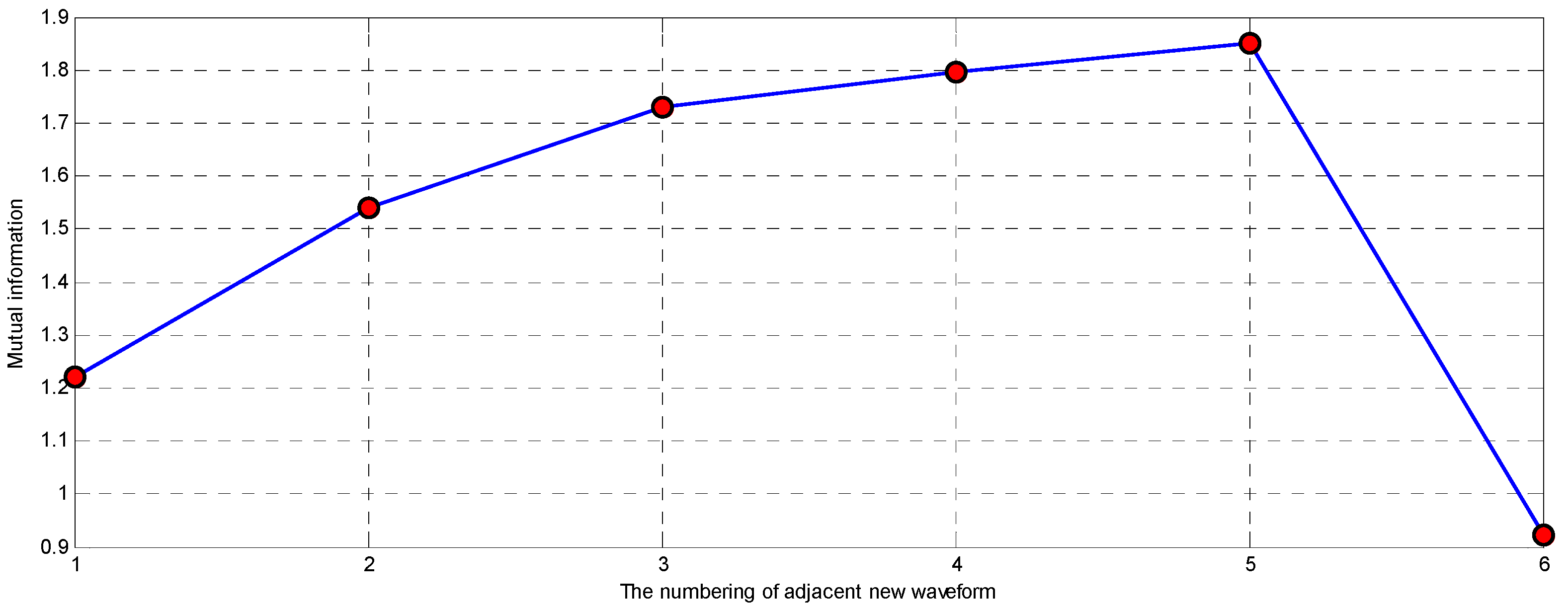
3.1. Mutual Information
3.2. Identification of Relevant Mode
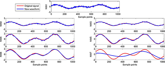
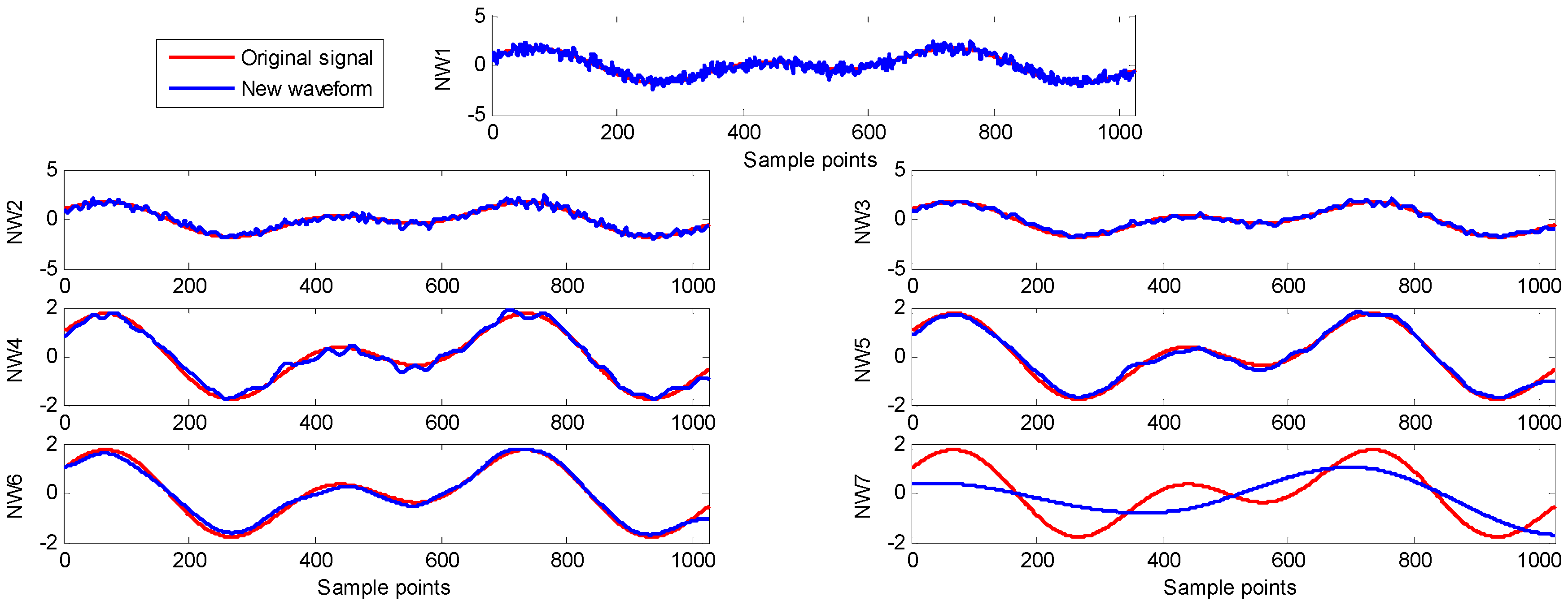
- (1)
- Obtain the new waveform by the difference between the original signal and the sum of IMFs, respectively.where N is total number of modes, IMFs are obtained by EMD or improved versions of decomposition, and is the n-th new waveform.
- (2)
- Calculate the mutual information of adjacent new waveforms:where is the abbreviation of mutual information.
- (3)
- Identify the index of the relevant mode:
- (4)
- Obtain the filtered signal:
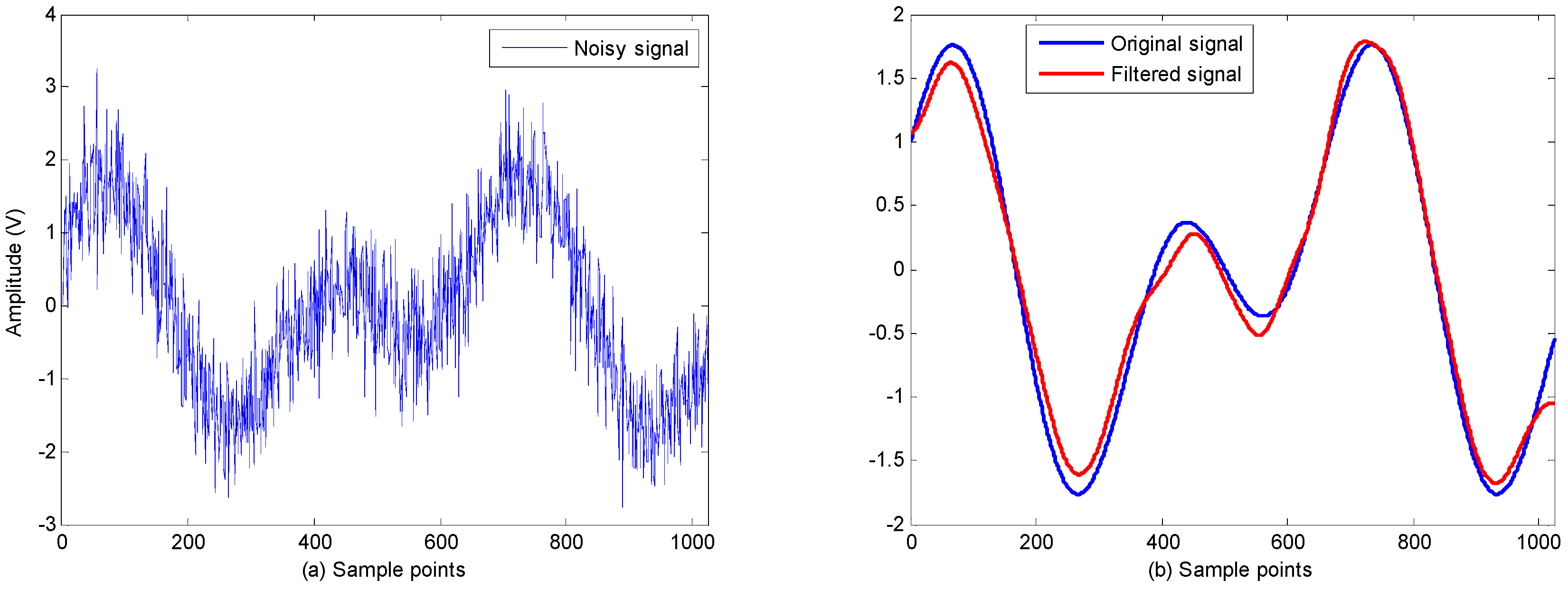
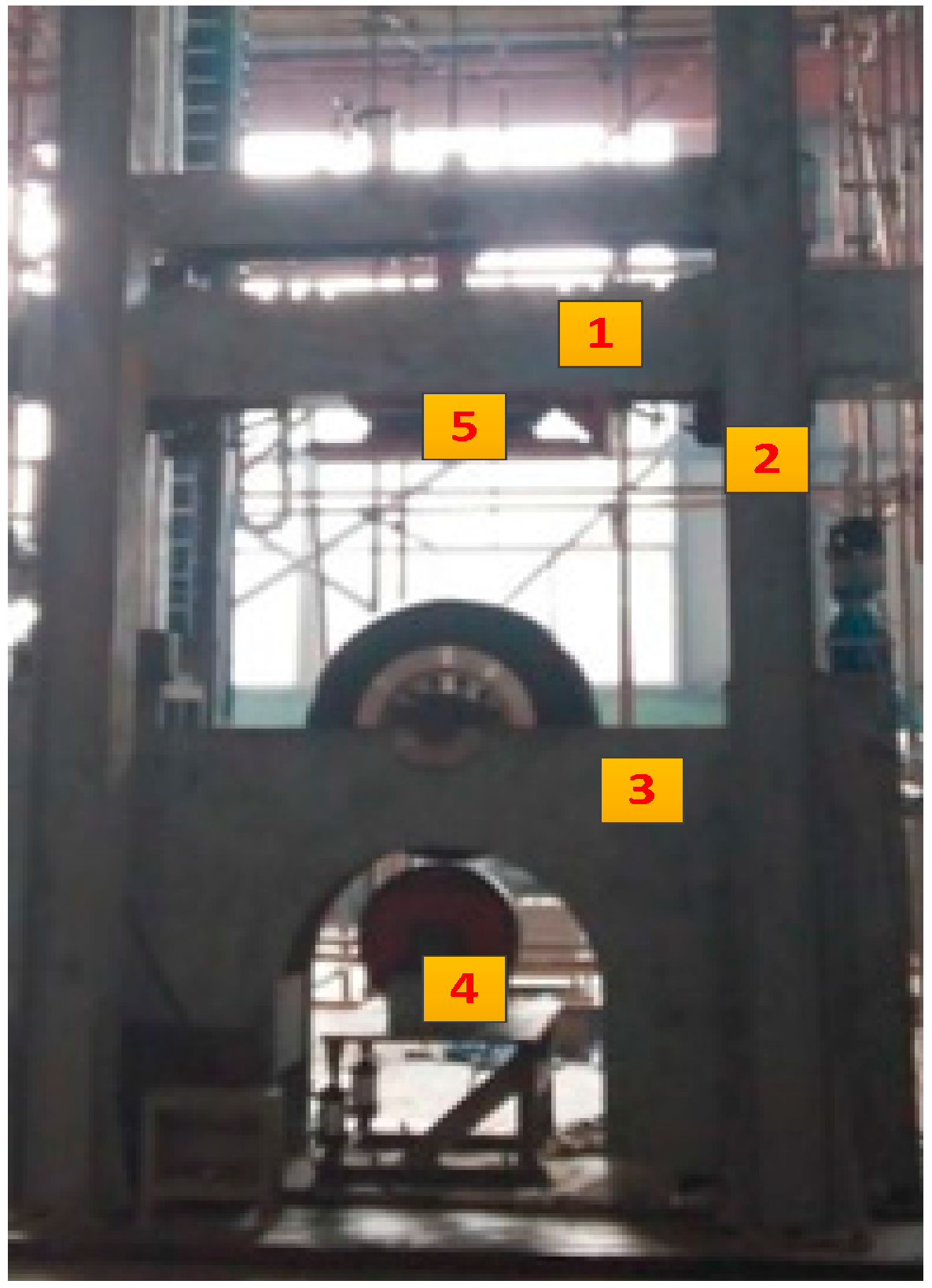
3.3. Application

4. Results and Discussions
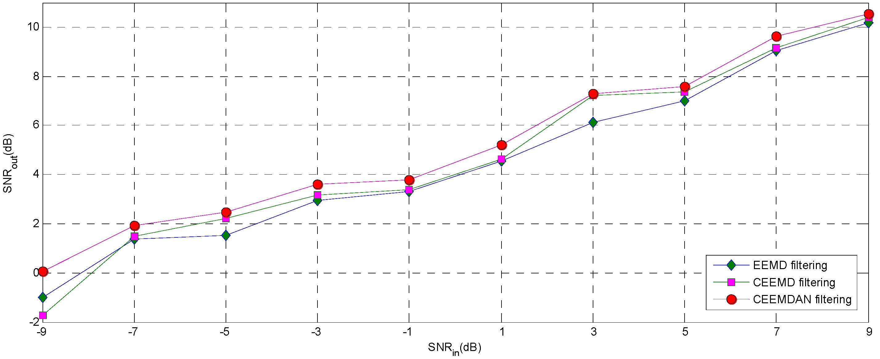
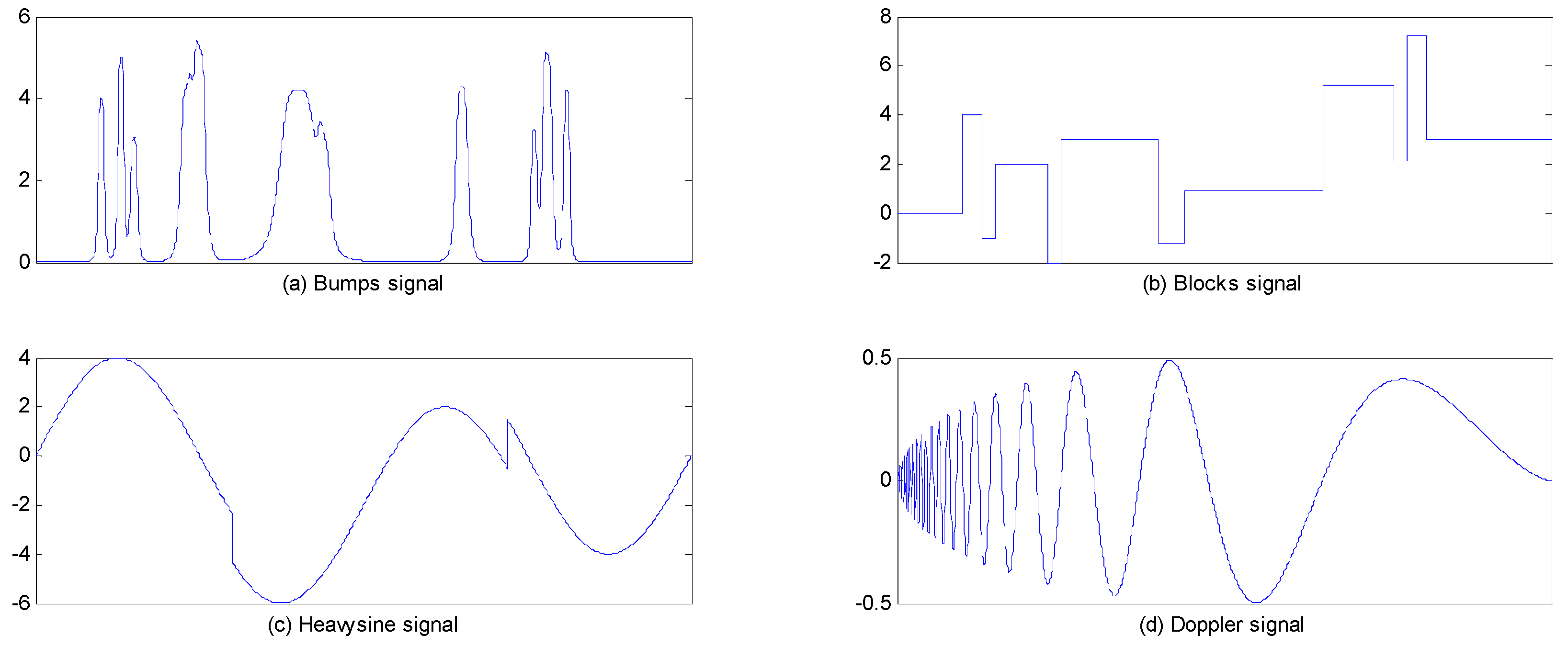
4.1. Simulation Signal Filtering
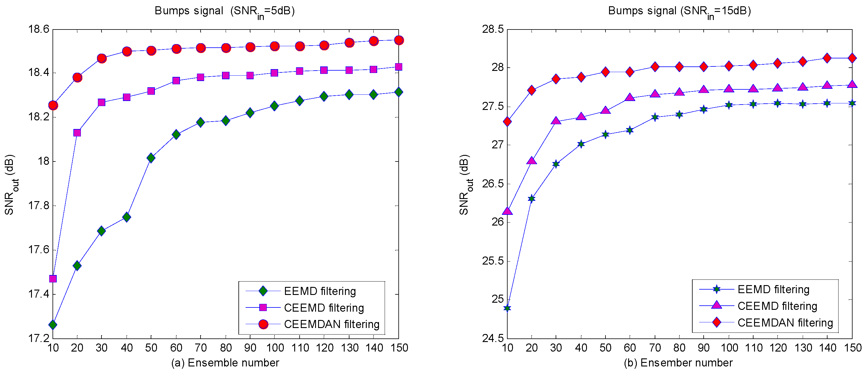
- (1)
- Compare by using a different ensemble number under the condition that the amplitude of the added white noise is the same.
- (2)
- Compare using a different sample rate.
- (3)
- Compare by adding a different input signal-noise ratios () into the original signal, where is the output signal-noise ratio.
4.1.1. Ensemble Number
4.1.2. Different Sampling Rate


4.1.3. Different Input Signal-Noise Ratio

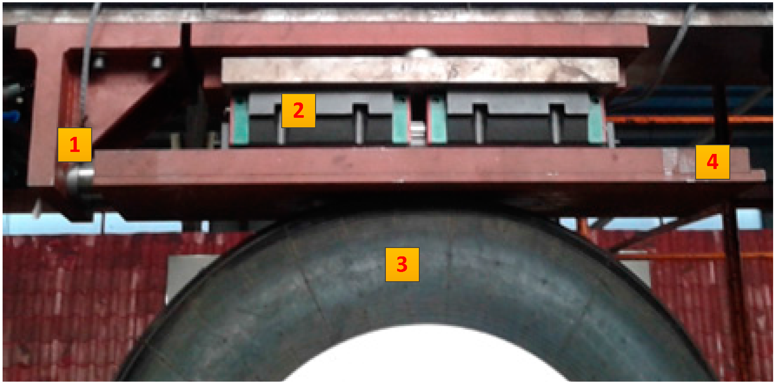
4.2. Friction Signal Filtering


- (1)
- Determine the integrated time series:where is the mean of time series .
- (2)
- Divide into n length segments;
- (3)
- Determine the local trend by using least squares method fitting;
- (4)
- Obtain fluctuation function by subtracting from the integrated time series ;
- (5)
- Get different through different length segments;
- (6)
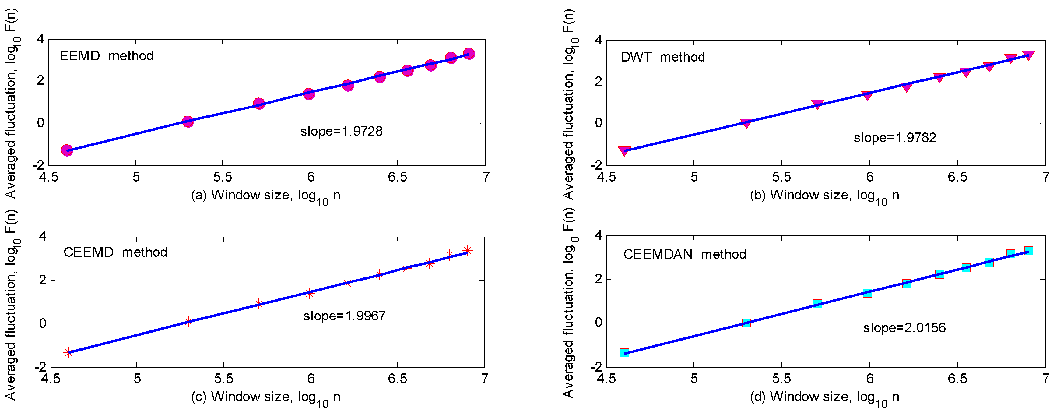
- Calculate the slope between and (the slope is called the fractal scaling index, represented as ), which is expressed by a power law as follows:
5. Conclusion
Author Contributions
Conflicts of interest
References
- Pacejka, H.B. Tyre and Vehicle Dynamics; Butterworth Heinenmann: Oxford, UK, 2002; pp. 97–104. [Google Scholar]
- Savkoor, A.R. On the friction of rubber. Wear 1965, 8, 222–237. [Google Scholar] [CrossRef]
- Pasterkamp, W.R.; Pacejka, H.B. The tyre as a sensor to estimate friction. Veh. Syst. Dyn. 1997, 27, 409–422. [Google Scholar] [CrossRef]
- Pasterkamp, W.R.; Pacejka, H.B. Optimal design of neural networks for estimation of tyre/road friction. Veh. Syst. Dyn. 1998, 29, 312–321. [Google Scholar] [CrossRef]
- Wang, R.; Wang, J. Tire-road friction coefficient and tire cornering stiffness estimation based on longitudinal tire force difference generation. Control Eng. Practice 2013, 21, 65–75. [Google Scholar] [CrossRef]
- Li, L.; Yang, K.; Jia, G.; Ran, X.; Song, J.; Han, Z.Q. Comprehensive tire-road friction coefficient estimation based on signal fusion method under complex maneuvering operations. Mech. Syst. Signal Process. 2015, 56, 259–276. [Google Scholar] [CrossRef]
- Proakis, J.G.; Mnaolakis, D.G. Digital Signal Processing: Principles, Algorithms, and Applications; Prentice-Hall: Englewood Cliffs, NJ, USA, 1996; pp. 223–229. [Google Scholar]
- Xia, R.; Meng, K.; Qian, F.; Wang, Z. Online wavelet denoising via a moving window. Acta Automatica Sinica 2007, 33, 897–901. [Google Scholar] [CrossRef]
- Donoho, D.L. De-noising by soft-thresholding. IEEE Trans. Inf. Theory 1995, 41, 613–627. [Google Scholar] [CrossRef]
- Huang, N.E.; Shen, Z.; Long, S.R.; Wu, M.C.; Shih, H.H.; Zheng, Q.; Yen, N.-C.; Tung, C.C.; Liu, H.H. The empirical mode decomposition and the Hilbert spectrum for nonlinear and non-stationary time series analysis. Proc. Roy. Soc. A math. Phys. Eng. 1998, 454, 903–995. [Google Scholar] [CrossRef]
- Flandrin, P.; Rilling, G.; Goncalves, P. Empirical mode decomposition as a filter bank. IEEE Signal Process. Lett. 2004, 11, 112–114. [Google Scholar] [CrossRef]
- Khaldi, K.; Boudraa, A.O.; Alouane, T.H. A new EMD denoising approach dedicated to voiced speech signals. In Proceedings of 2nd International Conference on Signals, Circuits and Systems, Monastir, Tunisia, 7–9 November 2008; pp. 1–5.
- Hadjileontiadis, L.J. A novel technique for denoising explosive lung sounds emnpirmical mode decompiosition and fractal dimension foilter. IEEE Eng. Med. Biol. Mag. 2007, 26, 30–39. [Google Scholar] [CrossRef] [PubMed]
- Tang, B.; Dong, S.; Song, T. Method for eliminating mode mixing of empirical mode decomposition based on the revised blind source separation. Signal Process. 2012, 92, 248–258. [Google Scholar] [CrossRef]
- Wu, Z.; Huang, N.E. Ensemble empirical mode decomposition: A noise-assisted data analysis method. Adv. Adapt. Data Anal. 2009, 1, 1–41. [Google Scholar] [CrossRef]
- Fang, Y.-M.; Feng, H.-L.; Li, J.; Li, G.-H. Stress Wave Signal Denoising Using Ensemble Empirical Mode Decomposition and an Instantaneous Half Period Model. Sensors 2011, 11, 7554–7567. [Google Scholar] [CrossRef] [PubMed]
- He, X.; Goubran, R.A.; Liu, X.P. Ensemble Empirical Mode Decomposition and adaptive filtering for ECG signal enhancement. In Proceedings of 2012 IEEE International Symposium on Medical Measurements and Applications (MeMeA), Budapest, Hungary, 18–19 May 2012; pp. 1–5.
- Yeh, J.-R.; Shieh, J.-S.; Huang, N.E. Complementary ensemble empirical mode decomposition: A novel noise enhanced data analysis method. Adv. Adapt. Data Anal. 2010, 2, 135–156. [Google Scholar] [CrossRef]
- Torres, M.E.; Colominas, M.A.; Schlotthauer, G.; Flandrin, P. A complete ensemble empirical mode decomposition with adaptive noise. In Proceedings of 2011 IEEE International Conference on Acoustics, Speech and Signal (ICASSP), Prague, Czech, 22–27 May 2011; pp. 4144–4147.
- Gan, Y.; Sui, L.; Wu, J.; Wang, B.; Zhang, Q.; Xiao, G. An EMD threshold de-noising method for inertial sensors. Measurement 2014, 49, 34–41. [Google Scholar] [CrossRef]
- Kabir, M.A.; Shahnaz, C. Denoising of ECG signals based on noise reduction algorithms in EMD and wavelet domains. Biomed. Signal Proces. 2012, 7, 481–489. [Google Scholar] [CrossRef]
- Shannon, C.E. A mathematical theory of communication. Bell Syst. Tech. J. 1948, 27, 379–423/623–656. [Google Scholar] [CrossRef]
- Chen, Z.; Hu, K.; Carpena, P.; Bernaola-Galvan, P.; Stanley, H.E.; Ivanov, P.C. Effect of nonlinear filters on detrended fluctuation analysis. Phys. Rev. E 2005, 71, 011104. [Google Scholar] [CrossRef]
- Chen, Z.; Ivanov, P.C.; Hu, K.; Stanley, H.E. Effect of nonstationarities on detrended fluctuation analysis. Phys. Rev. E 2002, 65, 041107. [Google Scholar] [CrossRef]
- Horvatic, D.; Stanley, H.E.; Podobnik, B. Detrended cross-correlation analysis for non-stationary time series with periodic trends. Europhysics Lett. 2011, 94, 18007. [Google Scholar] [CrossRef]
- Leistedt, S.; Dumont, M.; Lanquart, J.-P.; Jurysta, F.; Linkowski, P. Characterization of the sleep EEG in acutely depressed men using detrended fluctuation analysis. Clin. Neurophysiol. 2007, 118, 940–950. [Google Scholar] [CrossRef] [PubMed]
© 2015 by the authors; licensee MDPI, Basel, Switzerland. This article is an open access article distributed under the terms and conditions of the Creative Commons Attribution license (http://creativecommons.org/licenses/by/4.0/).
Share and Cite
Li, C.; Zhan, L.; Shen, L. Friction Signal Denoising Using Complete Ensemble EMD with Adaptive Noise and Mutual Information. Entropy 2015, 17, 5965-5979. https://doi.org/10.3390/e17095965
Li C, Zhan L, Shen L. Friction Signal Denoising Using Complete Ensemble EMD with Adaptive Noise and Mutual Information. Entropy. 2015; 17(9):5965-5979. https://doi.org/10.3390/e17095965
Chicago/Turabian StyleLi, Chengwei, Liwei Zhan, and Liqun Shen. 2015. "Friction Signal Denoising Using Complete Ensemble EMD with Adaptive Noise and Mutual Information" Entropy 17, no. 9: 5965-5979. https://doi.org/10.3390/e17095965
APA StyleLi, C., Zhan, L., & Shen, L. (2015). Friction Signal Denoising Using Complete Ensemble EMD with Adaptive Noise and Mutual Information. Entropy, 17(9), 5965-5979. https://doi.org/10.3390/e17095965