Prebiotic Competition between Information Variants, With Low Error Catastrophe Risks

Abstract

During competition for resources in primitive networks increased fitness of an information variant does not necessarily equate with successful elimination of its competitors. If variability is added fast to a system, speedy replacement of pre-existing and less-efficient forms of order is required as novel information variants arrive. Otherwise, the information capacity of the system fills up with information variants (an effect referred as “error catastrophe”). As the cost for managing the system’s exceeding complexity increases, the correlation between performance capabilities of information variants and their competitive success decreases, and evolution of such systems toward increased efficiency slows down. This impasse impedes the understanding of evolution in prebiotic networks. We used the simulation platform Biotic Abstract Dual Automata (BiADA) to analyze how information variants compete in a resource-limited space. We analyzed the effect of energy-related features (differences in autocatalytic efficiency, energy cost of order, energy availability, transformation rates and stability of order) on this competition. We discuss circumstances and controllers allowing primitive networks acquire novel information with minimal “error catastrophe” risks. We present a primitive mechanism for maximization of energy flux in dynamic networks. This work helps evaluate controllers of evolution in prebiotic networks and other systems where information variants compete.

1. Introduction

Most information used to manage living cells is encrypted in DNA and RNA sequences and expressed into order (i.e., nonrandom composition, organization and behavior) via transcription/translation machinery. One evolutionary outcome of encryption is that information variants (genes and gene clusters) compete with each other by proxy, i.e., via forms of order (or organized sub-systems) competing for resources such as materials and energy. One benefit of genetic memory is that diversity in information content (or virtual system states) can be larger than the diversity of types of order expressed at any given time. Furthermore, because of encryption, absence of expression does not by necessity imply loss in information content. On the contrary, in prebiotic networks that are too primitive to have a translation machinery (i.e., molecular automata), information is not encrypted, but explicit [1]. This means that some components may be simultaneously information carriers and forms of order. For example, according to some RNA-world theories, primitive cells could have existed with RNA-related molecules functioning as both genes and enzymes [2,3,4,5]. Such primitive RNA-like molecules and this type of primitive genetics is assumed to have existed before ribosomal translation has originated. These primitive RNA-like molecules contained conserved sequences, or sequence patterns. They can be described as genes because they store mutable information and because upon replication their sequence, or sequence pattern, can multiply. They can also be characterized as enzymes (or other functional components) because each specific RNA sequence (or sequence pattern) will fold in a specific 3D configuration that may act as an enzyme (or other functional components). Yet, internal competition for resources continues in such systems between various forms of order, and the survival of sequence information depends on expressing their physiological function. Consequently, when competition pushes one form of order to zero, its corresponding information variant is eliminated (an interesting form of prebiotic Lamarkian evolution).

In modern living systems, making changes from one controlled system state to another uses three main avenues: translating information from genetic memory; exchanging encrypted information with other systems; and evolution of existing information via mutation, variability and selection (MVS). The evolution of primitive networks that do not yet use cryptic information is largely dependent on MVS, but without the benefits of genetic memory. In such systems, balance has to exist between the rate of mutation and the selection of information variants. The overall rate of eliminating less-efficient information variants has to be equal to, or larger than, the rate of introducing novel information variants. Otherwise, the diversity of information variants (and internal forms of order) increases until carrying capacity is reached where the system’ complexity is too large for management. An analogous dilemma from RNA-world models was called “error catastrophe” [6].

The aim of this work is better understanding of how primitive networks used energy-related factors to efficiently screen out low-efficiency information variants, thus allowing information content to evolve with low “error catastrophe” risks. We have constructed a dynamic model of an isothermal system with finite material resources, in which two information variants (forms of order or sub-systems) called Syst#1 and Syst#2 compete (Figure 1).

Figure 1. Diagram of a system containing two information variants (types of order or sub-systems) called Syst#1 and Syst#2 competing for building materials (BM) and free energy (W) in a BM-finite environment. These sub-systems have similar cyclomatic complexity (v = 3). “nf” = Natural forward rate. “nr” = Natural reverse rate. The two sub-systems can be given dissimilar energy-related performance. Q = Heat released during energy dissipation. The model assumes an infinite heat sink in the exterior and no temperature variation. During simulations, changes in ratio between A and B components occur, as well as changes in abundance between the two sub-systems. One sub-system is considered to be over-competed when its relative abundance changes from 50% to < 1% in a given timeframe (i.e., full length simulation). The arrow indicated by the Autocatalyzed path shows the positive feedback of B units on the A => B transformation.

Figure 1. Diagram of a system containing two information variants (types of order or sub-systems) called Syst#1 and Syst#2 competing for building materials (BM) and free energy (W) in a BM-finite environment. These sub-systems have similar cyclomatic complexity (v = 3). “nf” = Natural forward rate. “nr” = Natural reverse rate. The two sub-systems can be given dissimilar energy-related performance. Q = Heat released during energy dissipation. The model assumes an infinite heat sink in the exterior and no temperature variation. During simulations, changes in ratio between A and B components occur, as well as changes in abundance between the two sub-systems. One sub-system is considered to be over-competed when its relative abundance changes from 50% to < 1% in a given timeframe (i.e., full length simulation). The arrow indicated by the Autocatalyzed path shows the positive feedback of B units on the A => B transformation.

These two sub-systems have similar cyclomatic complexity [7] and types of components and dissimilar composition and energy-related properties. The cyclomatic complexity of a network was defined by McCabe in 1976 as:

• v = e − n + 2p, where: v = the cyclomatic number of a network or circuit (a measure of its complexity);
• e = the number of edges in a network (equivalent with the number of connections, or avenues of transformation, between the various types of components from inside the network);
• n = the number of vertices in a network (equivalent to the number of types of components);
• p = the number of externally connected components (i.e., 2p is the number of entries and exits connecting the network with the exterior).

Adding properties to Syst#2 is equivalent to mutations influencing performance. A threshold for successful removal of Syst#1 has been established based on a hypothetical mutation rate. The model’s overall assumption is that the likelihood of “error catastrophe” is lowest if Syst#2 over-competes Syst#1 before new information variants arrive. Here, we only study factors that help Syts#2 succeed, and not consequences of adding more information variants. Effects of five energy-related parameters have been analyzed: (1) autocatalytic efficiency of order; (2) energy cost of order; (3) free energy availability; (4) transformation rate; and (5) stability of order. We asked: (1) How do these variables interact and influence competition between information variants?; (2) Is there a primordial “Goldilocks zone” (i.e., combination of variables) for low error catastrophe risk?; (3) How is this “zone” dependent upon environmental vs. internal factors?; and (4) Is there an evolutionary path that a primitive network can follow in order to avoid error catastrophe, by using internal variables subject to adaptive evolution?

2. Results and Discussion

2.1. Series 1

Using the model from Figure 1 we have analyzed how increased autocatalytic efficiency of B2 (“Autocat_B2” parameter in the model) influences the competitive success of Syst#2 as a function of energy availability (“free_E_input”) and free energy content of B2 entities (“EG_B2”). In this series, the intrinsic rate of transformation (“Ro”) is fixed. Its effects will be analyzed in Series 2. Since autocatalysis is a self-rewarding feature, it is expected that if “Autocat_B2” > “Autocat_B1”, then “A2:B2 ratio” < “A1:B1 ratio”. In turn, excess B2 is predicted to increase the natural B2 => A2 transformation rate, leading to higher energy costs for maintaining Syst#2 at disequilibrium. This series also aims determining how the range of “EG_B2” and the “free_E_input” influence competition between Syst#2 and Syst#1 at various “Autocat_B2” levels.

Figure 2 summarizes results of ~ 1,728 Stella simulations (32,000 steps each; DT = 1), using 32 values for “free_E_input” (in the 1×10⁻¹⁵ to ≈ 3×10⁻³ J range), nine values for “EG_B2” (in the 1.2×10⁻¹⁷ to ≈ 2.4×10⁻¹⁶ J range) and six values for “Autocat_B2” (in the 1.1 ≈ 4.0 range). In this series, it is assumed that the range of EG is smaller than the range of energy availability in the environment. Simulations have shown that if “Autocat_B2” = “Autocat_B1” and “EG_B2” ≤ “EG_B1”, Syst#2 cannot over-compete Syst#1 for any given “free_E_input” (results not shown). This is because without changes in autocatalysis, only the cost of order influences competition, and the overall system (Syst#1 + Syst#2) evolves toward the state of lowest order and free energy content (i.e., according to the 2^nd law of thermodynamics).

Figure 2. The evolution of competitive success of Syst#2 (“compet_success_2vs1”) in the model from Figure 1. The panels A through F represent variation for six values of autocatalytic activity of B2 components (“Autocat_B2”). “Autocat_B1” = 1 in all simulations. Each graph shows the effect of two variables: “free_E_input” (the availability of free energy in the exterior), and “EG_B2” (the free energy content per B2 component). The smallest value for EG used in these graphs (log(EG) = −16.92) corresponds with “EG_B2” = 1.2 × 10⁻¹⁷J. “EG_B1” = 6.6 × 10⁻¹⁷ J in all simulations. A single value for the standard rates of transformation has been used: “Ro_A1_to_B1” = “Ro_A2_to_B2” = 1×10⁻⁴. Each graph summarizes results of 288 Stella simulations with 32,000 steps each (DT = 1). The vertical axis shows the competitive success of Syst#2 at the end of each simulation. When “compet_success_2vs1” = 0, the mass of Syst#2 equals that of Syst#1. When “compet_success_2vs1” = 1, Syst#1 is eliminated. The wireframe on the 3D graph and on the 2D map projection on the XY axis distinguishes various colors (where: dark blue = −1; green = mid values around 0; highest red values = 0.98–0.99 and white > 0.99). We have selected white for the peak in competitive success of Syst#2 in order to obtain maximum contrast on the 2D XY projection. The white area in the 2D map projection shows cases where Syst#1 has reached ≤ 1% at the end of simulations.

Figure 2. The evolution of competitive success of Syst#2 (“compet_success_2vs1”) in the model from Figure 1. The panels A through F represent variation for six values of autocatalytic activity of B2 components (“Autocat_B2”). “Autocat_B1” = 1 in all simulations. Each graph shows the effect of two variables: “free_E_input” (the availability of free energy in the exterior), and “EG_B2” (the free energy content per B2 component). The smallest value for EG used in these graphs (log(EG) = −16.92) corresponds with “EG_B2” = 1.2 × 10⁻¹⁷J. “EG_B1” = 6.6 × 10⁻¹⁷ J in all simulations. A single value for the standard rates of transformation has been used: “Ro_A1_to_B1” = “Ro_A2_to_B2” = 1×10⁻⁴. Each graph summarizes results of 288 Stella simulations with 32,000 steps each (DT = 1). The vertical axis shows the competitive success of Syst#2 at the end of each simulation. When “compet_success_2vs1” = 0, the mass of Syst#2 equals that of Syst#1. When “compet_success_2vs1” = 1, Syst#1 is eliminated. The wireframe on the 3D graph and on the 2D map projection on the XY axis distinguishes various colors (where: dark blue = −1; green = mid values around 0; highest red values = 0.98–0.99 and white > 0.99). We have selected white for the peak in competitive success of Syst#2 in order to obtain maximum contrast on the 2D XY projection. The white area in the 2D map projection shows cases where Syst#1 has reached ≤ 1% at the end of simulations.

For small values of “Autocat_B2” (e.g., 1.1. in Figure 2 Panel A), and in general when “Autocat_B2” < 1.5, efficient elimination of Syst#1 did not occur (as competition success becomes saturated at small values), irrespective of the magnitude of the “free_E_input” and “EG_B2”. In Figure 2, Panel A, albeit B2-autocatalysis (= 1.1) is larger than B1-autocatalysis (= 1.0), situations do exist when Syst#1 is more successful than Syst#2. This effect occurs in a small free energy availability range (approximately 10⁻¹¹ to ≈ 10⁻¹⁰J) and when the energy cost of building B2 is large (log(EG) > −16.3). This phenomenon is due to autocatalysis not being sufficiently strong to favor the energy costly Syst#2 in an environment where energy availability is limiting. This phenomenon disappears when energy availability is very little (< 10⁻¹¹J), because insufficient free energy exists to build up disequilibrium in either system and the low cost Syst#1 prevails. It is also absent when free energy becomes more abundant, because the autocatalytic capability of Syst#2 finds sufficient energy for growth. In this model, the threshold where “Autocat_B2” becomes relevant is approximately 1.5. When “Autocat_B2” = 1.5 efficient elimination of Syst#1 occurs, yet only within very narrow range of energy availability, i.e., “free_E_input” between 1 × 10⁻¹⁰ and 2 × 10⁻¹⁰J (Figure 2; Panel B), and when the energy content of order “EG_B2” ≤ 10^−16.5J.

Below this range, the competitive success of Syst#2 diminishes because insufficient free energy is present in the environment to maintain a large excess of B2. Above this range, the B2 autocatalysis is unable to absorb all free energy from the exterior, and residual free energy helps Syst#1 survive longer. As “Autocat_B2” increased however, (e.g., in the 1.6 to ≈ 2.0 range), the range of energy availability where efficient elimination of Syst#1 occurred has also broadened (Figure 2, Panels C–E). At “Autocat_B2” = 4, Syst#2 over-competed Syst#1 over a wide range of energy availability and B2 energy content. At low “Autocat_B2” (=1.5 to ≈ 1.75) the competitive success of Syst#2 has decreased with “EG_B2” (Figure 2. Panels B–D). For “Autocat_B2” ≥ 1.5 this effect is not seen in the figure because the EG range displayed in the graph is too little. Yet, this effect remains and was verified for “EG_B2” up to 1.2 × 10⁻¹⁴ J (results not shown). This effect is due to high energy costs for building B2 entities relative to advantages of autocatalysis, and decreases at large energy availability.

2.2. Series 2

This series analyzes the effect of “Autocat_B2” on competition between Syst#2 and Syst#1 for various levels of energy availability (“free_E_input”) and A⇔B exchange rates (“Ro_Ax_to_Bx”). A single value for “EG_B2” = 4.2 × 10⁻¹⁷J was used, corresponding to “Irs” = 40 and “kG” = 3 × 10⁻¹⁸J/bit (this EG value is in the range from Series 1, Figure 2). Increase in the A⇔B rate is equivalent with the activity of a catalyst, and “Ro_Ax_to_Bx” modifications do not alter the A:B ratio at equilibrium, but shorten the time needed to reach it. Combining larger A⇔B rate with larger B2 autocatalysis is expected to increase the turnover time of building materials through the B2 reservoir and to also increase the energy cost of maintaining order afar from equilibrium. Faster A⇔B exchange can also be produced by increase in temperature, but this would also influence the BM⇔A exchange rate. In this series, only the A⇔B transformation rates are modified, not the BM⇔A rates as well. Very slow A⇔B rates are expected to diminish access of B structures to building materials before they are exchanged back between A and BM. Very fast A⇔B rates are expected to shorten the residence time of building materials in the B reservoir, giving competitors a chance to pick them up through the BM reservoir. Figure 3 summarizes results of 1,344 Stella simulations (each 32,000 steps long; DT = 1).

Figure 3. The evolution of competitive success of Syst#2 (“compet_success_2vs1”) in the model from Figure 1. Panels A through F represent variation for six values of autocatalytic activity of B2 components (“Autocat_B2”). “Autocat_B1” = 1 in all simulations. Each graph shows the effect of two variables: “free_E_input” (the exterior free energy availability), and the intrinsic rate of A⇔B transformations (“Ro_Ax_to_Bx”), representing the contribution of a catalyst of the A⇔B transformation. Panels A through F use the same range and values for “Autocat_B2” and “free_E_input” from Figure 2. The −5 value on the log(Ro_Ax_to_Bx) axis represents natural uncatalyzed transformation. All other graph notations and color code are similar to Figure 2.

Figure 3. The evolution of competitive success of Syst#2 (“compet_success_2vs1”) in the model from Figure 1. Panels A through F represent variation for six values of autocatalytic activity of B2 components (“Autocat_B2”). “Autocat_B1” = 1 in all simulations. Each graph shows the effect of two variables: “free_E_input” (the exterior free energy availability), and the intrinsic rate of A⇔B transformations (“Ro_Ax_to_Bx”), representing the contribution of a catalyst of the A⇔B transformation. Panels A through F use the same range and values for “Autocat_B2” and “free_E_input” from Figure 2. The −5 value on the log(Ro_Ax_to_Bx) axis represents natural uncatalyzed transformation. All other graph notations and color code are similar to Figure 2.

Figure 3 simulations have shown that efficient competition between two information variants only occurs within a specific range of A⇔B transformation rate and of energy availability, and that the relationship between variables and competitive success is complex and difficult to predict (Figure 3, Panels B–E). As autocatalysis of order increases however, competitive success of Syst#2 becomes more predictable over wide range of energy availability and A⇔B rate. For “Autocat_B2” ≥ 2 the zone of competitive efficiency for Syst#2 is broad. This is important because “Autocat_B2” = 2 is but a modest upgrade in autocatalytic efficiency (and subject to adaptive evolution), yet makes competition between information variants stringent, and predictable over broad range of energy conditions.

2.3. Series 3

In this series, parameters have the same range as in Series 1 (Figure 2) but increase in order is also associated with lower decay rate, which extends the time needed for the A⇔B system to reach equilibrium. Results summarizing 1526 Stella8^® (see Experimental Section for details), simulations (32,000 steps each) are shown in Figure 4. The general trend showing consequences of increasing “Autocat_B2” remains, but with a few differences. Unlike Figure 2, Panel A (“Autocat_B2” = 1.1), “compet_success_2vs1” never reaches negative values. At small autocatalytic efficiency the increased stability of B2 makes Syst#2 “lose less ground” relative to Syst#1 (Figure 4, Panel A). This shows that as ordered systems gain stability and autocatalytic capabilities, chances for success in competition improve and beneficial environmental niches can extend to broad range of energy availability. The stability of structures also plays an important role in competitive success. For example, increased stability of B2 entities led to improvement in competitive success of Syst#2 at lower energy levels than in Series 1. Increased stability of order also allowed small changes in autocatalysis influence the efficiency of information selection. When autocatalytic efficiency was large (“Autocat_B2” = 4) increase in the stability of order diminished the upper limit where excess energy availability has lowered the efficiency of Syst#2 (Figure 4, Panel F). This series of simulations shows how increased capacity of Syst#2 to sequester energy, and primarily the ability of a sub-system to adjust its energy dissipative activity to energy availability, can help eliminate competitors by starvation.

Figure 4. The evolution of competitive success of Syst#2 (“compet_success_2vs1”) in the model from Figure 1. Variables from each graph are similar to those from Figure 2, but in this series of simulations larger “EG_B2” value also increases the stability of order. Each graph summarizes the results of 256 Stella simulations with 32,000 steps each (DT = 1). All other graph notations and color code are similar to Figure 2.

Figure 4. The evolution of competitive success of Syst#2 (“compet_success_2vs1”) in the model from Figure 1. Variables from each graph are similar to those from Figure 2, but in this series of simulations larger “EG_B2” value also increases the stability of order. Each graph summarizes the results of 256 Stella simulations with 32,000 steps each (DT = 1). All other graph notations and color code are similar to Figure 2.

3. Experimental Section

The model analyzed in this paper (Figure 1), is an example of “abstract chemistry”, wherein properties of participating components are more important than their identity as real world objects. One rationale for using abstract chemistry is that finding properties various components should have for explaining the origin of life in a given environment and timeframe, is preferable to screening libraries of all possible chemicals from a hypothetical environment to surmise if, and how, may they help explain the origin of life. Another, is that abstract models are non-Earth-centric in that they help study principles of prebiotic organization that, putatively, apply to wide variety of life forms irrespective of composition, structure, size, scale, rate of activity and type of habitat. Many artificial life platforms exist that satisfy abstract chemistry requirements and can be used to construct origin of life models [10,11,12,13,14,15,16,17,18]. The one selected for this study is Biotic Abstract Dual Automata (BiADA) [19,20,21,22]. The software we have used is Stella8^® (http://www.iseesystems.com/softwares/Education/StellaSoftware.aspx), and the file (written in Stella) is available at www.ksg.ro/Entropy_simulation02.STM. Principles of BiADA modeling, the meaning of various parameters, equations, sequence of commands, model limitations and technical solutions have been previously published [19,20]. Next, we summarize BiADA principles and model parameters used in this study.

Building materials (BM) and organized structures (e.g., A1, A2, B1 and B2, see Figure 1) from BiADA models are virtual objects. Since they do not represent specific chemicals or other physical objects they can be assigned any property with regard to mass, amount, composition, thermodynamic values, information capacity, specificity of interaction with other components and transformation kinetics. All components of similar type make up a stock (or population). Components and stocks only contain integer number of parts. Transfer of components, energy and information between stocks are called flows. Flows occur in steps (or cycles) and each step only involves integer number of components or component parts. The amount of components transferred between stocks in each step is the integer of a calculated value, yet limited to the size of the source stock. A stock can only contain zero or positive number of components and no negative values occur in the model. A BiADA model uses the following set of rules, explained in more detail previously [20]:

(1)

Each type of component in a BiADA model is characterized by two energy-related features, free energy content and heat content;

(2)

Each type of component is characterized by two information-related features: Residual information and Remanent information. Residual information is the unused information capacity in a system or the information capacity of the disordered part of the system. Remanent information is the information capacity removed due to ordering the system. The sum between Residual information and Remanent information is called Virtual information and represents the maximum information capacity of a system (or Shannon’s information capacity) in the fully disordered state.

(3)

The parameters representing free energy, heat content, Residual information and Remanent information are only given zero or positive values; and thermodynamic rules of transformation are obeyed.

(4)

All transformations are integer increments or decrements of building blocks and are expressed in units of transformation.

(5)

All transformations or transfer of materials and energy between internal components are uni-flows (i.e., forward and reverse transformations are analyzed separately). Natural and catalyzed flows are also analyzed separately. In BiADA models equilibrium is determined by differences between forward and reverse transformations.

(6)

The direction and equilibrium of a process is derived from differences between the net forward and net reverse transformations.

The model functions as follows: after stocks and flows are designed, all equations are written, all components receive values regarding energy and information content and the rates of all transformations are established. These values influence the magnitude of the flows. Catalytic functions are added to various parts of the model and influence transformation rates. The first step in a BiADA simulation is to assign to each stock (i.e., BM, A1, A2, B1 and B2) an initial number of components. Then free energy is added to the system and the model runs for 32,000 steps. During each run, we have monitored the evolution of the size of each stock and calculated the competitive success of Syst#2.

The names for various parameters used in this paper are identical with parameter notations from the software; this allows users to easily identify and manipulate variables. The model parameters used in this paper are:

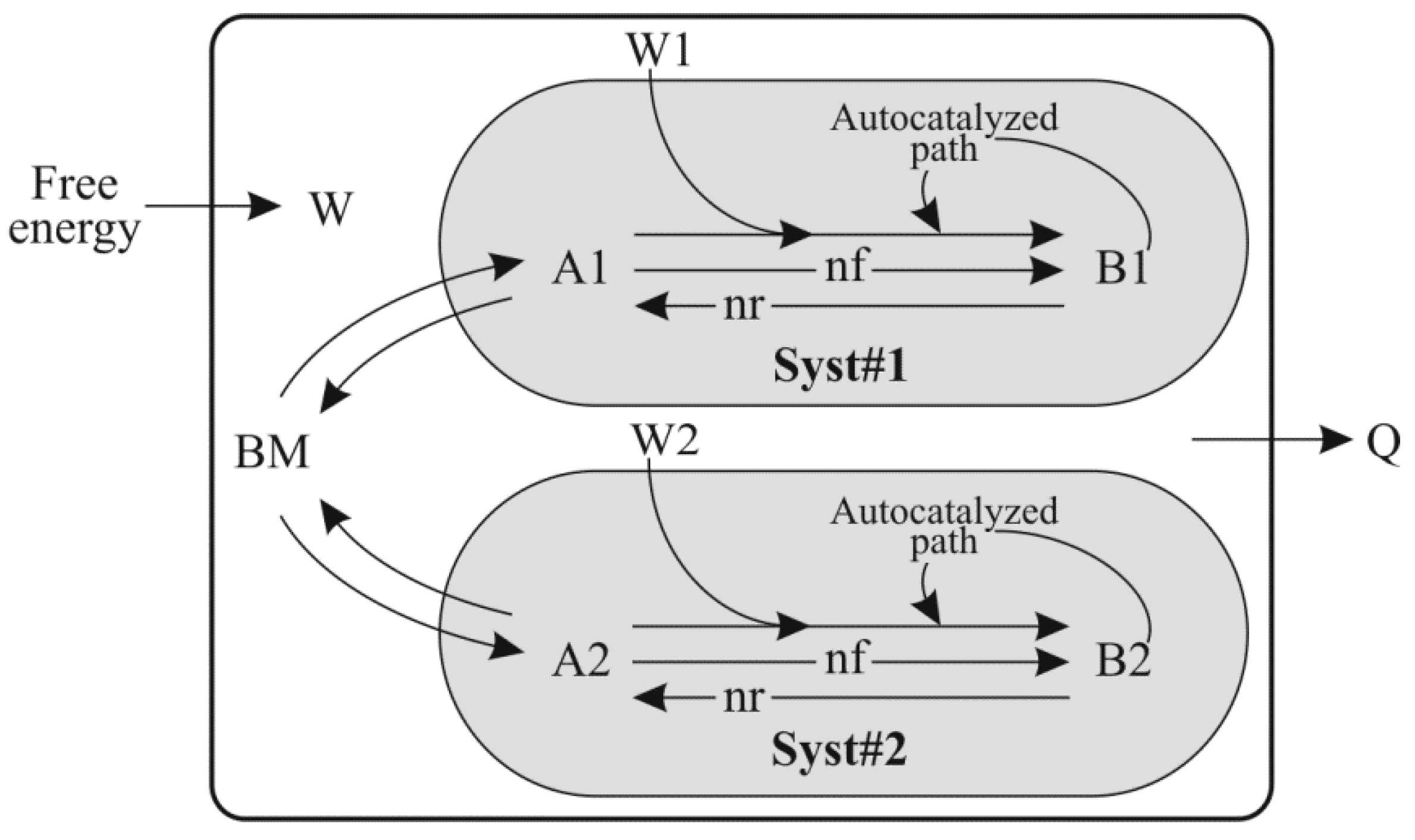
• “Init_BM_units”, “Init_A1_units”, “Init_B1_units”, “Init_A2_units” and “Init_B2_units” represent the amount of various components used in the model (BM, A1, B1, A2 and B2 respectively) at the beginning of a simulation.
• “BM”, “A1”, “B1”, “A2” and “B2” are the magnitude of the five stocks used in this model (Figure 1), expressed in mass units.
• “Irs_BM_units”, “Irs_A1_units”, “Irs_B1_units”, “Irs_A2_units” and “Irs_B2_units” are the residual information capacity of the entities “BM”, “A1”, “B1”, “A2” and “B2”, respectively. Irs represents the information capacity present in a system or structure after ordering has removed degrees of freedom. The capacity of Irs (expressed in bits) indicates the amount of information that can still be stored in the system by further ordering.
• “Irm_BM_units”, “Irm_A1_units”, “Irm_B1_units”, “Irm_A2_units” and “Irm_B2_units” are the remanent information content of the entities “BM”, “A1”, “B1”, “A2” and “B2” respectively. Irm, means information content and represents the amount of information capacity removed by ordering the system.
• “Ivt_BM_units”, “Ivt_A1_units”, “Ivt_B1_units”, “Ivt_A2_units” and “Ivt_B2_units” are the virtual information content of the entities “BM”, “A1”, “B1”, “A2” and “B2” respectively. Ivt is the information capacity of the system in fully disordered state, and Ivt = Irs + Irm.
• “kG_of_BM_J_per_bit_Irm”, “kG_of_A1_J_per_bit_Irm”, “kG_of_B1_J_per_bit_Irm”, “kG_of_ A2_J_per_bit_Irm” and “kG_of_B2_J_per_bit_Irm” are the free energy associated with one bit of Irm in the “BM”, “A1”, “B1”, “A2” and “B2” entities respectively. kG is variable, as free energy content relative to Irm varies among various ordered structures.
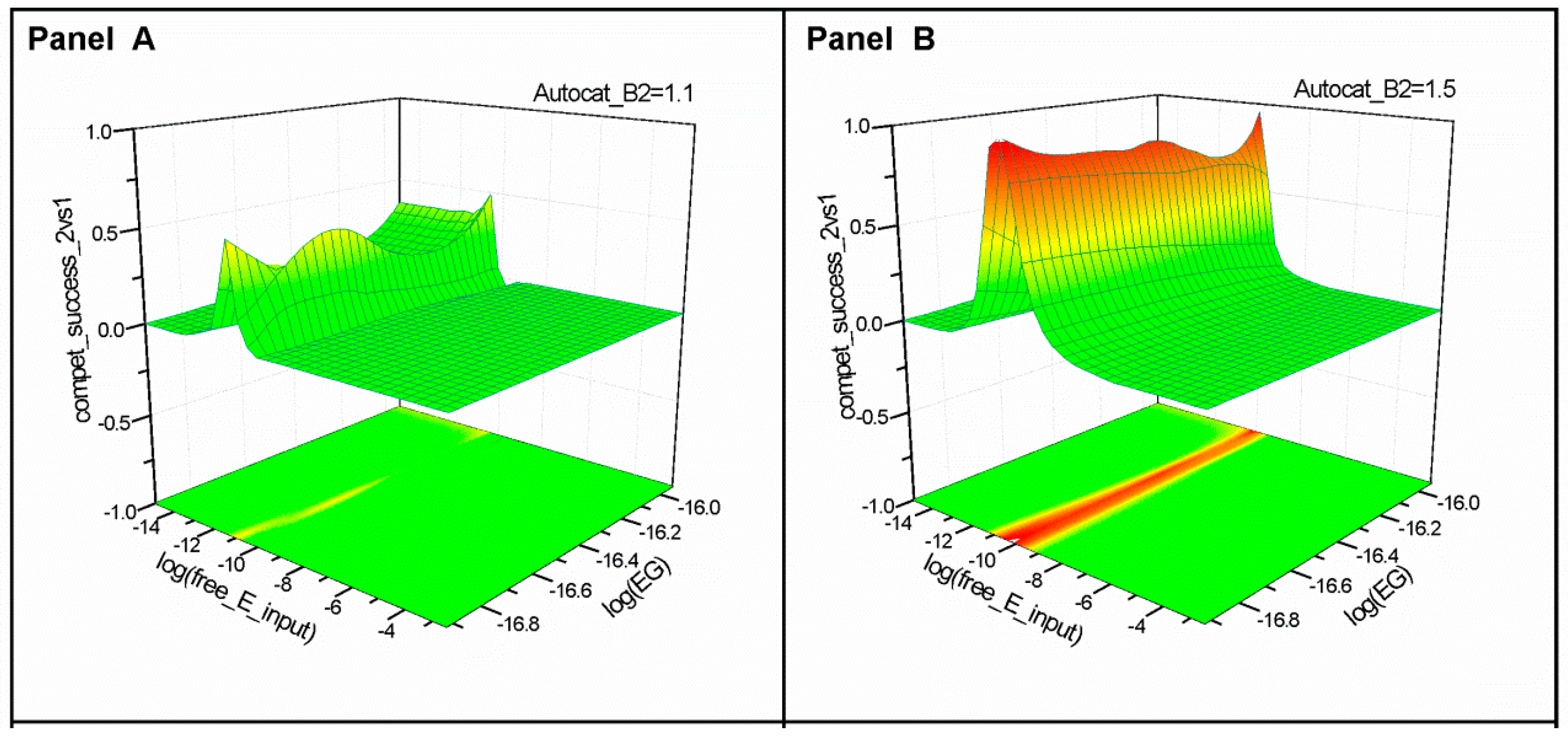
• “EG_BM_J_per_unit_transf”, “EG_A1_J_per_unit_transf”, “EG_B1_J_per_unit_transf”, “EG_A2_ J_per_unit_transf” and “EG_B2_J_per_unit_transf” are the free energy associated with units of transformation of “BM”, “A1”, “B1”, “A2” and “B2”, respectively. EG = kG × Irm. EG is equivalent to the free energy content of an organized structure. In the model, the value of EG of an organized structure can be modified by increasing the order of a structure (Irm) or its kG value.
• “free_E_input” is the availability of free energy in the environment.
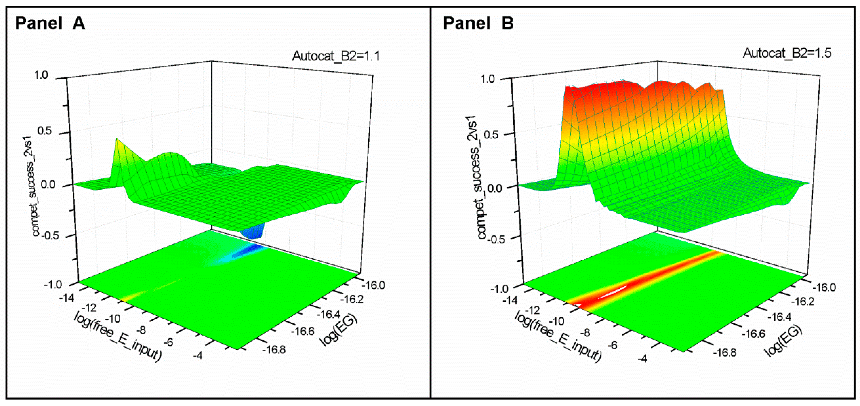
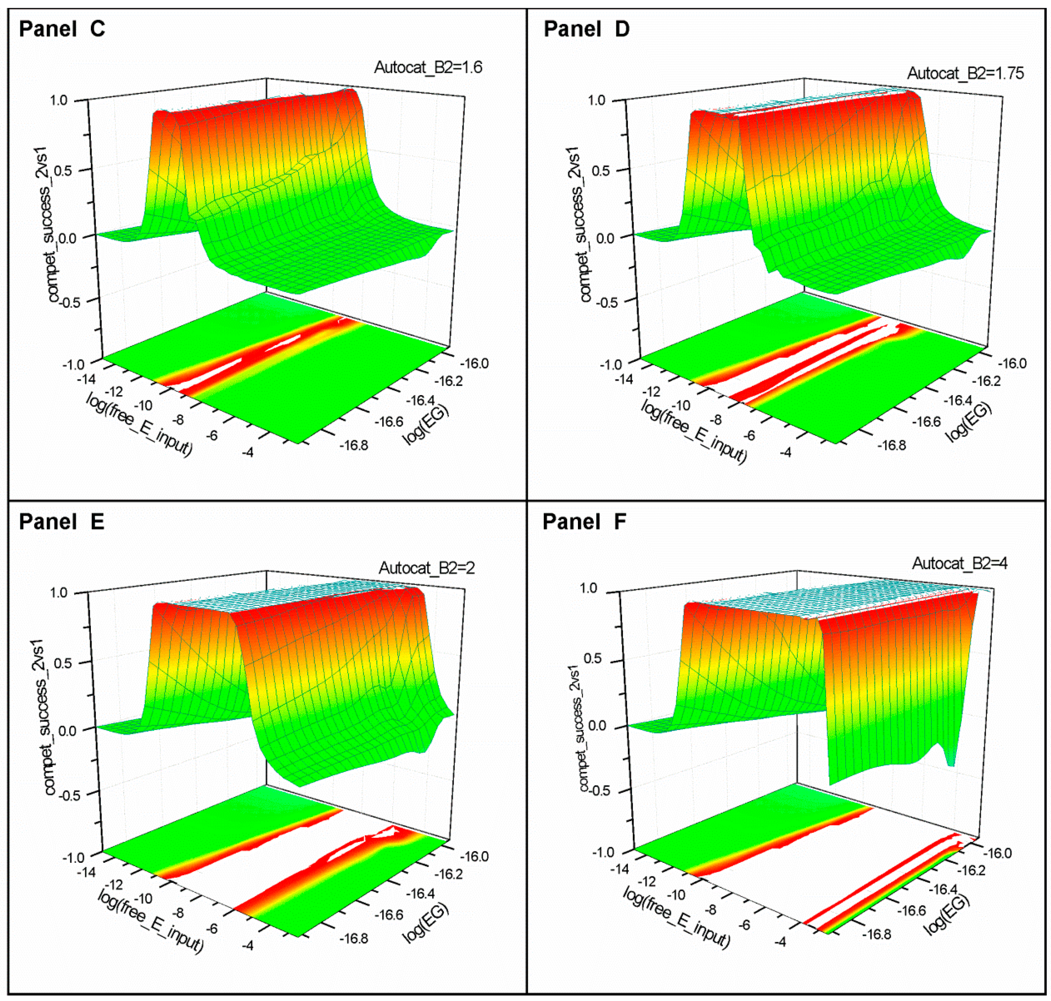
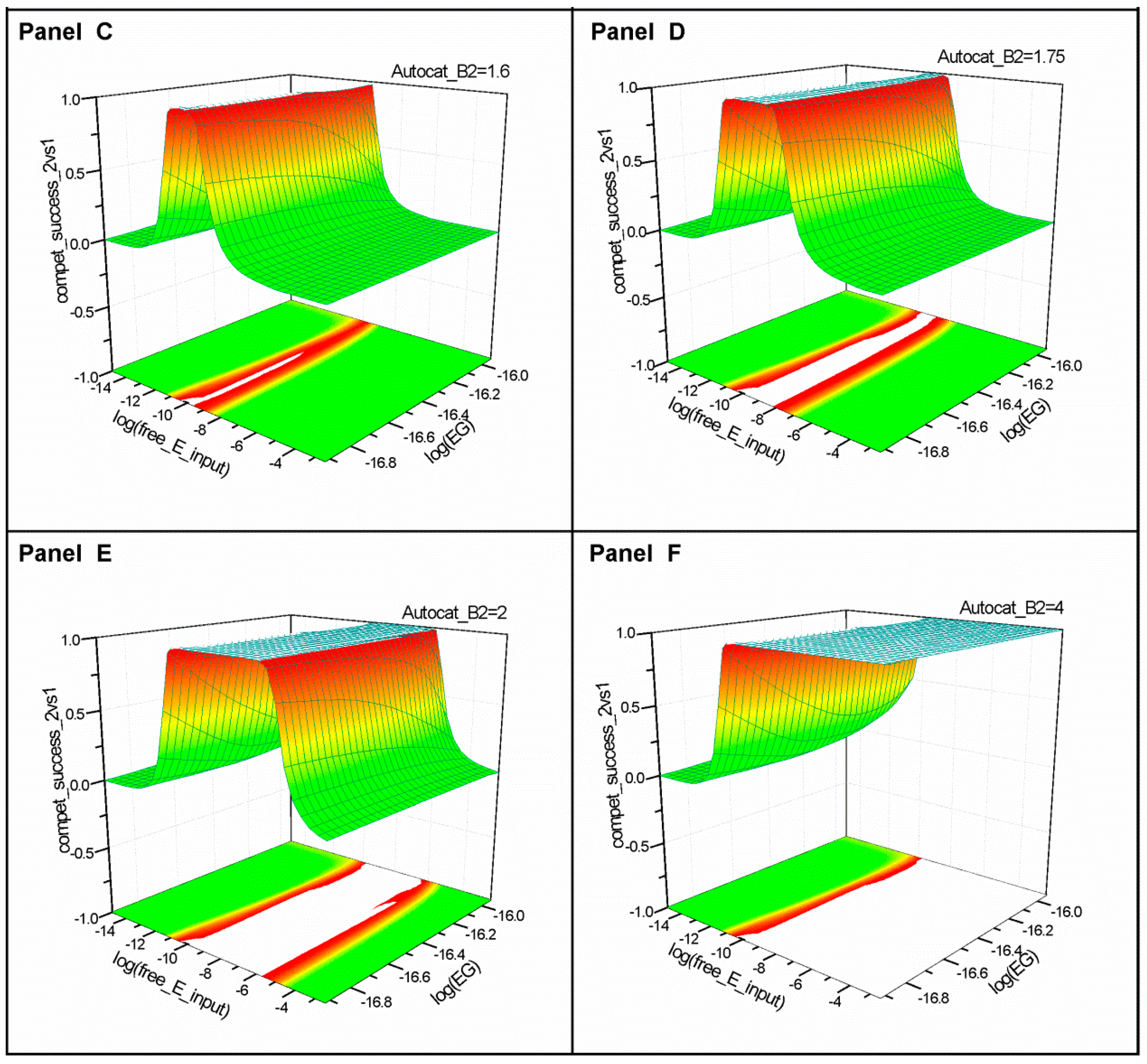
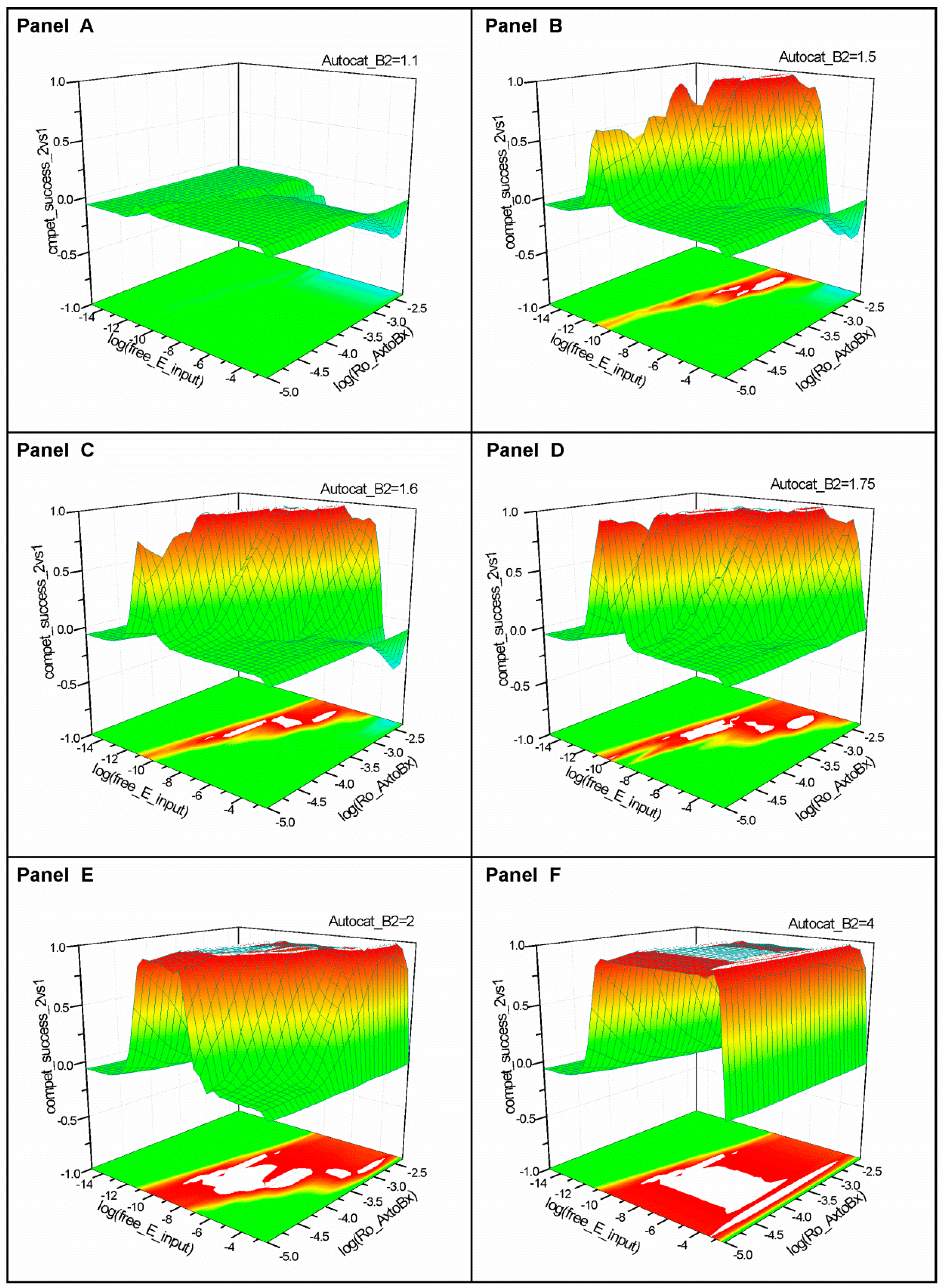
• “Autocat_B1” and “Autocat_B2” are the autocatalytic capability of the entities B1 and B2 respectively. “Autocat” is ≥ 0. The rate of the Autocatalyzed path in Syst#1 from Figure 1 is proportional to the magnitude of the B1 stock at the power of “Autocat_B1”; same formula is used for the rate of the Autocatalyzed path in Syst#2.
• “Ro_BM_to_A1”, “Ro_A1_to_B1”, “Ro_BM_to_A2” and “Ro_A2_to_B2” are the intrinsic rates of forward transformations: “BM to A1”, “A1 to B1”, “BM to A2” and “A2 to B2”, respectively.
• “Ro_A1_to_BM”, “Ro_B1_to_A1”, “Ro_A2_to_BM” and “Ro_B2_to_A2” are the intrinsic rates of reverse transformations: “A1 to BM”, “B1 to A1”, “A2 to BM” and “B2 to A2”, respectively.
• “Compet_success_2vs1” = ((A2 + B2) − (A1 + B1))/(A1 + B1 + A2 + B2) measures the dominance of Syst#2 over Syst#1 during competition. Total elimination of Syst#1 is often not observed within reasonable timeframe (i.e., 32,000 simulation steps). An efficient competition-success threshold has been established as the ability of Syst#2 to reach 99% abundance during 32,000 step simulation for Delta Time (DT) = 1.

All other BiADA parameters present in the model file, but not used in this paper, have been explained in earlier publications [19,20,21,22]. Based on the requirements of a particular simulation, parameters and rules in a model may be used in totality of partly. For example in this paper we do not monitor the evolution of heat content and the variation of temperature in the system. In the model from Figure 1, the “A” structures are more complex and have larger EG and Irm per unit mass than the “BM” structure, and the “B” structures are more complex and have larger EG and Irm per unit mass than “A”. Natural flows between “BM” and “A” and between “A” and “B” are assumed to only require kinetic energy and energy from fundamental forces. Increase in order (such as departure from equilibrium toward larger abundance of “B”, relative to the expected natural “A:B” equilibrium, requires free energy.

4. Conclusions

We have analyzed the effect of energy-related variables on the selection of information variants competing inside primitive networks. Results indicate that information variants gain little in lieu of competitive efficiency if differences in autocatalytic efficiency are small. This is most likely because the range of energy availability where information selection is stringent is narrow. On the contrary, large differences in autocatalytic efficiency (analogous to anastrophes [23]) between information variants, greatly extend the energy availability range where selection is stringent. We report one of the simplest primeval mechanisms for making a system adjust (i.e., increase) its energy dissipation to energy availability. This mechanism is based on a combination between autocatalysis (amplification of existing order) and temperature-independent increase in forward and reverse transformation rates (i.e., conventional catalysis). Maximizing the energy flux increases competitive success of an information variant, because it allows some sub-systems exploit free energy more efficiently. It is postulated that in the early evolution of dynamic networks, if autocatalytic performance was poor, the most important controller of efficient screening of information variants was environmental, i.e., inhabiting niches with narrowly specified and “just right” energy availability. Subsequently, as autocatalytic performance has increased the screening rate of information variants became more influenced by internal factors. These include managing energy costs of order and increased energy dissipative potential. Tolerance of stringent selection among information variants to broad energy availability has also increased.

It is proposed that during very early evolution of prebiotic networks, elimination of less-fit information competitors was inefficient in energy poor, energy copious and energy variable environments. Initial increase in system performance and order was slow and depended on narrow match between the efficiency of autocatalysis and energy availability in the environment. The driver for such networks to evolve toward increased complexity was “progressive increase in energy availability”. In more evolved networks, synergism between autocatalysis and transformation kinetics increased the energy dissipative potential. This helped more-efficient information variants “starve” their competitors and transferred control over information screening rate to internal parameters. Adjusting energy flux to energy availability has amplified quality differences between information variants, has allowed prebiotic evolution to progress in small increments and has minimized “error catastrophe” risks. In this paper we did not study the effect of cooperation between information variants because the system analyzed here (Figure 1) only contains two types of competing information variants and no exchange of information exists between the two types of systems. In future models, analyzing cooperation will be very important however.

References and Notes

1. Popa, R. Between Necessity and Probability: Searching for the Definition and Origin of Life; Springer: Berlin, Germany, 2004. [Google Scholar]
2. Shelley, D.C.; Smith, E.; Morowitz, H.J. The Origin of the RNA World: Co-evolution of Genes and Metabolism. Bioorgan. Chem. 2007, 35, 430–443. [Google Scholar]
3. Gilbert, W. Origin of Life: The RNA World. Nature 1986, 319, 618. [Google Scholar] [CrossRef]
4. Poole, A.M.; Jeffares, D.C.; Penny, D. The Path from the RNA World. J. Mol. Evol. 1998, 46, 1–17. [Google Scholar] [CrossRef] [PubMed]
5. Joyce, G.F. The Antiquity of RNA-Based Evolution. Nature 2002, 418, 214–221. [Google Scholar] [CrossRef] [PubMed]
6. Eigen, M. Self-organization of Matter and Evolution of Biological Macro-molecules. Naturwissenschaften. 1971, 58, 465–523. [Google Scholar] [CrossRef] [PubMed]
7. McCabe, T.J., Sr. A Complexity Measure. IEEE Trans. Softw. Eng. 1976, 4, 308–320. [Google Scholar] [CrossRef]
8. Dyson, F.J. A Model for the Origin of Life. J. Mol. Evol. 1982, 18, 344–350. [Google Scholar] [CrossRef] [PubMed]
9. Dyson, F.J. Origins of Life; Cambridge University Press: Cambridge, UK, 1999. [Google Scholar]
10. Rosen, R. On the Dynamical Realization of (M, R)-Systems. Bull. Math. Biol. 1973, 35, 1–9. [Google Scholar] [PubMed]
11. Ray, T.S. Evolution and Optimization of Digital Organisms. In Scientific Excellence in Supercomputing: The IBM 1990 Contest Prize Papers; Billingsley, K.R., Derohanes, E., Brown, H., Eds.; Baldwin Press: Boston, MA, USA, 1991; pp. 489–531. [Google Scholar]
12. Fontana, W.; Buss, L.W. What Would Be Conserved if the Tape Were Played Twice? Proc. Natl. Acad. Sci. USA 1994, 91, 757–761. [Google Scholar] [CrossRef] [PubMed]
13. Pargellis, A.N. The Evolution of Self-replicating Computer Organisms. Physica. D 1996, 98, 111–127. [Google Scholar] [CrossRef]
14. McMullin, B. SCL: An Artificial Chemistry in Swarm. Available online: http://samoa.santafe.edu/media/workingpapers/97-01-002.pdf (accessed on 23 July 2015).
15. Adami, C. Introduction to Artificial Life; Springer: Berlin, Germany, 1997. [Google Scholar]
16. Moran, F.; Moreno, A.; Minch, E.; Montero, F. Further Steps toward a Realistic Description of the Essence of Life. In Artificial Life V: Proceedings of the Fifth International Workshop on the Synthesis and Simulation of Living Systems (Complex Adaptive Systems); Langton, C.G., Shimonara, K., Eds.; MIT Press: Cambridge, MA, USA, 1997; pp. 255–263. [Google Scholar]
17. Bedau, M.A.; McCaskill, J.S.; Packard, N.; Rasmussen, S.; Adami, C.; Green, D.G.; Ikegami, T.; Kaneko, K.; Ray, T.S. Open Problems in Artificial Life. Artif. Life 2000, 6, 363–376. [Google Scholar] [CrossRef] [PubMed]
18. Wilensky, U.; Rand, W. NetLogo 3.1: Low Threshold, no Ceiling. Available online: https://ccl.northwestern.edu/papers/2006/SoftwareDemo.pdf (accessed on 23 July 2015).
19. Cimpoiasu, V.M.; Popa, R. Biotic Abstract Dual Automata (BIADA)−A Novel Tool for Studying the Evolution of Prebiotic Order (and the Origin of Life). Astrobiology 2012, 12, 1123–1134. [Google Scholar] [CrossRef] [PubMed]
20. Cimpoiasu, V.M.; Popa, R. Elimination of Less-Fit Information Variants during Competition between Low Complexity Dynamic Systems. Phys. AUC 2014, 24, 130–151. [Google Scholar]
21. Popa, R.; Cimpoiasu, V.M. Energy-Driven Evolution of Prebiotic Chiral Order (Lessons from Dynamic Systems Modeling). In Genesis—In the Beginning; Springer: Berlin, Germany, 2012; Volume 22, pp. 526–545. [Google Scholar]
22. Popa, R.; Cimpoiasu, V.M. Analysis of Competition between Transformation Pathways in the Functioning of Biotic Abstract Dual Automata. Astrobiology 2013, 13, 454–464. [Google Scholar] [CrossRef] [PubMed]
23. Baltscheffsky, H. Major “Anastrophes” in the Origin and Early Evolution of Biological Energy Conversion. J. Theor. Biol. 1997, 187, 495–501. [Google Scholar] [CrossRef] [PubMed]