Projective Synchronization of Chaotic Discrete Dynamical Systems via Linear State Error Feedback Control

Abstract

A projective synchronization scheme for a kind of n-dimensional discrete dynamical system is proposed by means of a linear feedback control technique. The scheme consists of master and slave discrete dynamical systems coupled by linear state error variables. A kind of novel 3-D chaotic discrete system is constructed, to which the test for chaos is applied. By using the stability principles of an upper or lower triangular matrix, two controllers for achieving projective synchronization are designed and illustrated with the novel systems. Lastly some numerical simulations are employed to validate the effectiveness of the proposed projective synchronization scheme.

1. Introduction

Nearby trajectories of a chaotic system may experience exponential divergence, but two or more coupled dissipative chaotic systems evolving in synchrony might appear quite surprising. Furthermore the synchronization error system between the coupled chaotic systems may be asymptotically stable if some suitable control techniques are implemented on them. As a common multi-disciplinary phenomenon, chaos synchronization has broad range applications, such as secure communication [1], chaotic economic systems [2], WINDMI systems [3], hyperchaotic complex-variable systems [4], chaotic complex networks [5], fractional-order chaotic neural networks [6], etc.

Fujisaka and Yamada [7], and Pecora and Carroll [8] did some pioneering works for chaos synchronization. Mainieri and Rehacek [9] first proposed the chaos projective synchronization scheme in 1999, but it was still very difficult to achieve projective synchronization between two or more chaotic nonlinear systems until Wen et al. [10,11] presented an observer-based control scheme for projective chaos synchronization in 2004, whose prominent advantage is “no special limitation” for nonlinear dynamical systems to achieve projective chaos synchronization. Wen and co-authors also tried to explore the potential applications of projective synchronization to noise reduction in mechanical engineering [12,13], design bifurcation solutions [14,15] and so on.

Projective chaos synchronization has been an active research topic in nonlinear science. A variety of control methods for projective chaos synchronization have been proposed for various kinds of nonlinear chaotic systems. Li et al. [16] proposed a backstepping control method to achieve adaptive function projective synchronization for a general class of the so-called strict-feedback chaotic discrete systems. Vasegh and Majd [17] presented a Takagi–Sugeno fuzzy model-based adaptive approach to synchronize two different chaotic discrete-time systems. Zhang et al. [18] designed an impulsive controller to achieve impulsive lag synchronization for a class of chaotic discrete systems. Zhang and Liu [19] presented an active robust model predictive control strategy for the synchronization of two discrete-time chaotic systems. Unfortunately, the aforementioned synchronization schemes are very complex and difficult to realize in the real world. In many real fields, there is an urgent need for us to develop, at least so far, a kind of simple and robust projective chaos synchronization schemes. Fortunately, the advantage of the linear feedback controller is that it is robust and linear, and moreover, it is easier to design and implement for chaos synchronization than the abovementioned schemes. Odibat et al. [20] studied synchronization for 3-dimensional chaotic fractional-order systems via linear control. Chen et al. [21,22] also did some sound work designing controllers which are less than the number of dimensions of the chaotic systems. By using linear state error feedback control technology, Xin et al. [2,3,23] studied the projective synchronization for three kinds of chaotic fractional-order systems. It is not difficult for us to extend the mentioned projective synchronization scheme from fractional-order systems to discrete dynamical systems.

The remainder of this paper is structured as follows: in Section 2, a novel discrete dynamical system is proposed and a 0–1 test algorithm for chaos is redescribed. In Section 3, a synchronization scheme for n-dimensional chaotic discrete dynamical systems is proposed. In Section 4, the proposed projective synchronization scheme is applied to the novel discrete dynamical systems. Numerical simulations are conducted in Section 5 to illustrate the proposed synchronization scheme. Finally, the paper is concluded in Section 6.

2. A Novel Discrete Dynamical System and 0–1 Test for Chaos

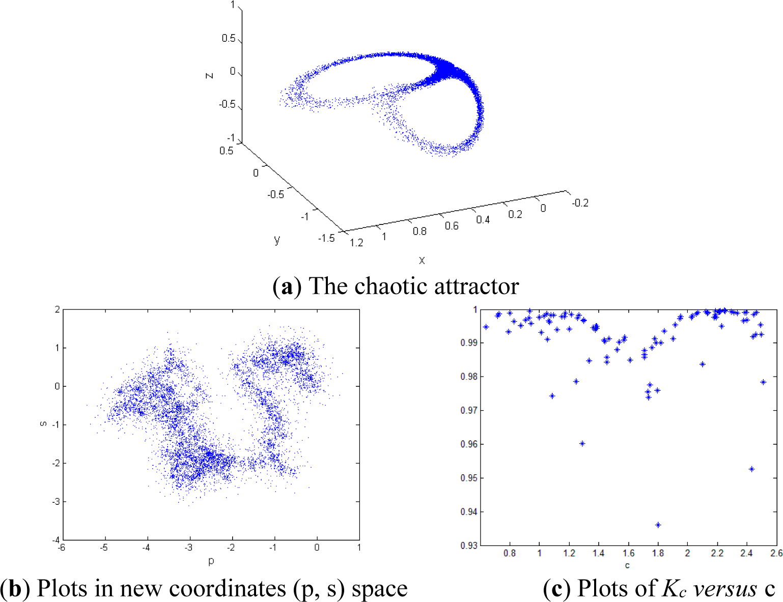
2.1. A Novel 3-D Discrete Dynamical System

To demonstrate mentioned projective chaos synchronization scheme, we first construct a novel 3-dimensional chaotic discrete dynamical system as follows:

$$\{\begin{array}{l}x(t+1)=-y(t)+a{x}^2(t),\\ y(t+1)=-bx(t)+\widehat{c}\mathrm{y}(t)-z(t)-x(t)z(t),\\ z(t+1)=-dz(t)+x(t)\mathrm{y}(t),\end{array}$$

(1)

where a, b, ĉ, d ≥ 0.

2.2. 0–1 Test Algorithm for Chaos

To identify the chaos existence of system (1), the 0–1 test algorithm for chaotic discrete dynamical system need redescription as follows [24–26]: consider the iteration times n =1, 2, ⋯, N as the sampling times in discrete dynamical system (10), where N is the total number of data points and ϕ(n) is an observable data, one can get a discrete time series ϕ(1), ϕ(2) ⋯, ϕ(N). The 0–1 test for chaos may be directly applied to the time series because there are no issues with oversampling:

• Step 1. Determine a random number c ∈ (π/5, 4π/5), and construct a pair of new coordinates (p_c (n), s_c (n)) as follows:

  $$p_c(n)={\displaystyle \sum _{j=1}^n\varphi (j)\cos (\theta (j)),}$$

  (2)

  $$s_c(n)={\displaystyle \sum _{j=1}^n\varphi (j)\sin (\theta (j)),}$$

  (3)

  Where:

  $$\theta (j)=jc+{\displaystyle \sum _{i=1}^j\varphi (j),j=1,2,\cdots ,n.}$$

  (4)
• Step 2. Define the mean square displacement M_c (n) as follows:

  $$M_c(n)=\underset{N\to \infty }{\lim }\frac{1}{N}{\displaystyle \sum _{j=1}^N\left[{\left(p_c(j+n)-p_c(j)\right)}^2+{\left(s_c(j+n)-s_c(j)\right)}^2\right],n\in \left[1,\frac{N}{10}\right].}$$

  (5)
• Step 3. Define the modified mean square displacement D_c (n) as follows:

  $$D_c(n)=M_c(n){\left[\underset{N\to \infty }{\lim }\frac{1}{N}{\displaystyle \sum _{j=1}^N\varphi (j)}\right]}^2\frac{1-\cos nc}{1-\cos c},$$

  (6)
• Step 4. Define the median value of correlation coefficient as follows:

  $$K=median({\mathrm{K}}_c),$$

  (7)

  where:

  $$K_c=\frac{\mathrm{cov}(\xi ,\mathrm{\Delta })}{\sqrt{\mathrm{var}(\xi )\mathrm{var}(\mathrm{\Delta })}}\in \left[-1,1\right],$$

  (8)

  where ξ = (1, 2, ⋯, n_cut) Δ = (D_c(1), D_c(2), ⋯, D_c(n_cut)), n_cut = round (N/10), and the covariance and variance are defined with vectors x, y of length q as follows:

  $$\mathrm{cov}(\mathrm{x},\mathrm{y})=\frac{1}{q}{\displaystyle \sum _{j=1}^q\left(x(j)-\overline{x}\right)\left(y(j)-\overline{y}\right)},$$

  (9)

  $$\overline{x}=\frac{1}{q}{\displaystyle \sum _{j=1}^{q}x(j)},$$

  (10)

  $$\mathrm{var}(x)=\mathrm{cov}(x,x).$$

  (11)
• Step 5. Interpret the outputs as follows:

  • K ≈ 0 implies that the underlying dynamics is regular (i.e., periodic or quasi-periodic), whereas K ≈1 implies that the underlying dynamics is chaotic;
  • Bounded trajectories in the (p, s)-plane indicate that the underlying dynamics is regular, whereas the Brownian-like (unbounded) trajectories indicate that the underlying dynamics is chaotic.

As a binary test for chaos detection for deterministic dynamical systems, the 0–1 test is very simple but powerful. However, as stated in Ref. [24], in the case of periodic dynamics, most values of c yield K_c = 0 as expected, but there are isolated values of c for which K_c is large due to resonances: for such a c we expect M_c (n) ~ n², irrespective of whether the dynamics is regular or chaotic. The occurrence of resonances for isolated values of c suggests using the median of the computed values of K_c as K = median (K_c). To get various values K_c versus c, 100 choices of c is sufficient in practice [25].

The chaos phenomenon is shown in Figure 1. The chaotic attractors are respectively plotted in the original state spaces (x, y, z) and in the transformed coordinates variables (p, s), as shown in Figures 1a,b, accordingly. Brownian-like (unbounded) trajectories shown in Figure 1b denote there is a chaotic attractor in system (1). Figure 1c is the plots of correlation coefficient K_c vs. random number c, which shows the median value K ≈ 1 implies that there exists chaotic dynamics in system (1).

3. A Synchronization Scheme of n-Dimensional Chaotic Discrete Dynamical Systems

Definition 1. The projective synchronization is defined as the difference between two relative chaotic dynamical systems can approach to zero when time approaches to infinity with a desired scaling factor.

Consider a chaotic discrete dynamical system as follows:

$$x(t+1)=L(x(t))+N(x(t))+C$$

(12)

where C is an n×1 constant matrix, x = (x₁, x₂, ⋯, x_n)^T ∈ ℝⁿ is an n-dimensional state vector of system (12), and L, N: ℝⁿ → ℝⁿ are linear and nonlinear functions of states respectively.

Correspondingly, one may construct the following discrete dynamical system:

$$y(t+1)=L(y(t))+k(N(x(t))+C)+u(t)$$

(13)

where y = (y₁, y₂, ⋯, y_n)^T ∈ ℝⁿ is an n-dimensional state vector of system (13), k is a desired scaling factor, and u(t) is a linear state error feedback controller.

Defining the synchronization error between the master system (12) and the slave system (13) as follows:

$$e(t)=y(t)-kx(t),i=1,2,\cdots ,n$$

(14)

The linear state error feedback controller u(t) is defined as:

$$u(t)=\widehat{A}e(t)$$

(15)

where  is an n × n linear constant matrix.

Subtracting (12) from (13), one get the following error system:

$$e(t+1)=y(t+1)-kx(t+1)=Le(t)+u(t)=Ae(t)$$

(16)

where A = L + Â is an n × n linear constant matrix. Obviously the original point is the equilibrium point of system (16).

Using the stability criterion of linear discrete dynamical systems, one may directly get the following theorem:

Theorem 1. If A is an upper or lower triangular matrix and all eigenvalues simultaneously satisfy |λ₁|, |λ₂|, ⋯, |λ_n| <1, then the fixed point of synchronization error e(t) is asymptotically stable and$\underset{t\to \infty }{\lim }(t)=0$, i.e., systems (12) and (13) achieve projective synchronization.

4. Application to the Novel Discrete Dynamical System

In order to analyze the projective synchronization behaviors of master-slave systems, one may regard system (1) as the master system and construct the slave system (denoted by the subscript s) as follows:

$$\{\begin{array}{l}{x}_s(t+1)=-y_s(t)+ka{x}^2(t)+{\mathrm{u}}_1(\mathrm{t}),\\ y_s(t+1)=-b{x}_s(t)+\widehat{c}{\mathrm{y}}_s(t)-{\mathrm{z}}_s(t)-kx(t)\mathrm{z}(t)+{\mathrm{u}}_2(\mathrm{t}),\\ z_s(t+1)=-d{\mathrm{z}}_s(t)+kx(t)\mathrm{y}(t)+{\mathrm{u}}_3(\mathrm{t}),\end{array}$$

(17)

where, x_s, y_s, z_s ∈ ℝ have the same meanings as x, y, z of system (1), k is a desired scaling factor, u₁, u₂, u₃ are linear state error feedback controllers.

Proposition 1. If anyone of the two following control laws holds, the master-slave systems (1) and (17) will finally achieve global projective synchronization for any initial condition:

$$\{\begin{array}{l}{u}_1=h_1(x_s-kx),\\ u_2=b(x_s-kx)+h_2(y_s-ky),\\ u_3=h_3(z_s-kz),\end{array}$$

(18a)

or:

$$\{\begin{array}{l}{u}_1=h_1(x_s-kx)+(y_s-ky),\\ u_2=h_2(y_s-ky)+(z_s-kz),\\ u_3=h_3(z_s-kz),\end{array}$$

(18b)

where |h₁| <1, |h₂ + ĉ| <1, |h₃ – d| <1.

Proof. One can define the synchronization errors between the master-slave systems (1) and (17) as follows:

$$\{\begin{array}{l}{e}_1=x_s-kx,\\ e_2=y_s-ky,\\ e_3=z_s-kz.\end{array}$$

Subtracting systems (17) from (1), one can get the error system as follows:

$$\{\begin{array}{l}{e}_1(t+1)=-e_2(t)+u_1(\mathrm{t}),\\ e_2(t+1)=-b{e}_1(\mathrm{t})+\widehat{c}{e}_2(\mathrm{t})-e_3(\mathrm{t})+u_2(\mathrm{t}),\\ e_3(t+1)=-d{e}_3(\mathrm{t})+u_3(t),\end{array}$$

(19)

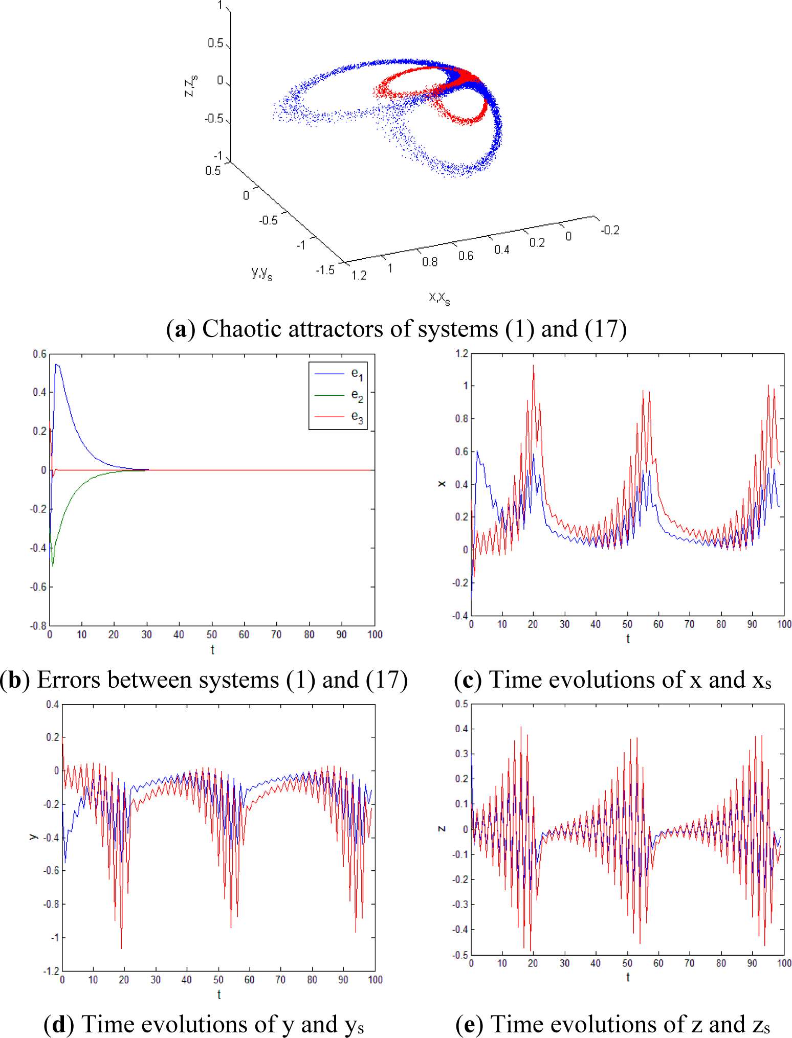
• Case 1:
  For the first control law in Proposition 1, substituting Equation (18a) into the error system (19), one can get the following error system:

  $$\{\begin{array}{l}{e}_1(t+1)=h_1{e}_1(\mathrm{t})-e_2(t),\\ e_2(t+1)=(h_2+\widehat{c})e_2(\mathrm{t})-e_3(\mathrm{t}),\\ e_3(t+1)=(h_3-d)e_3(\mathrm{t}),\end{array}$$

  (20)

  which has only one equilibrium point at E^* = (0,0,0). Evaluating its Jacobian matrix at E^*, one can get the upper triangular matrix as follows:

  $$J(E^{*})=\left(\begin{array}{ccc}{h}_1& -1& 0\\ 0& h_2+\widehat{c}& -1\\ 0& 0& h_3-d\end{array}\right),$$

  (21)

  whose eigenvalues simultaneously satisfy λ₁ = |h₁| <1, λ₂ = |h₂ + ĉ| <1 and λ₃ = |h₃ – d| <1.
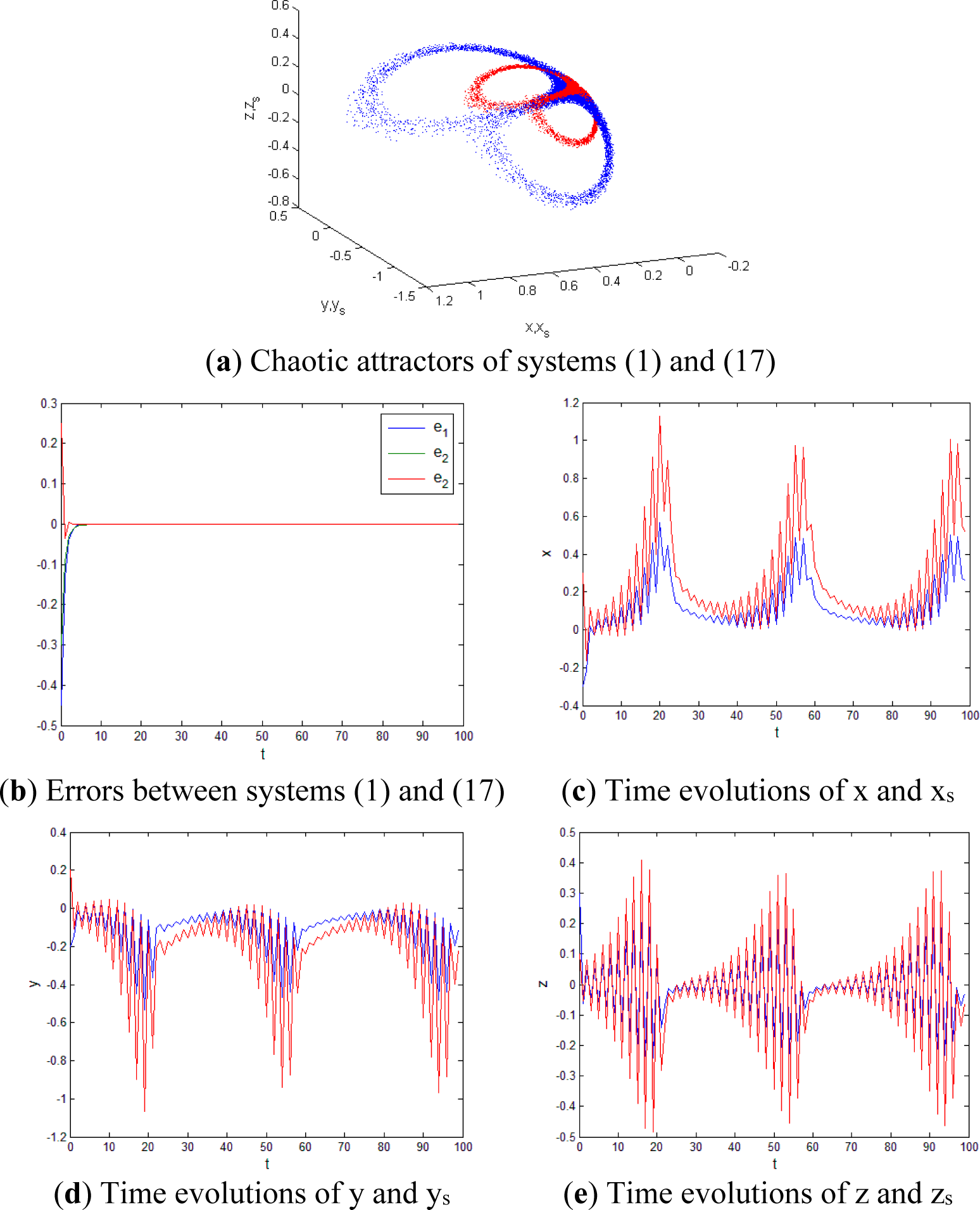
• Case 2:
  For the second control law in Proposition 1, substituting Equation (18b) into the error system (20), the system (20) can be re-depicted as follows:

  $$\{\begin{array}{l}{e}_1(t+1)=h_1{e}_1(\mathrm{t}),\\ e_2(t+1)=-b{e}_1(t)+(h_2+\widehat{c})e_2(\mathrm{t}),\\ e_3(t+1)=(h_3-d)e_3(\mathrm{t}),\end{array}$$

  (22)

  which has only one equilibrium point at E^* = (0,0,0). Evaluating its Jacobian matrix at E^*, one can get the lower triangular matrix as follows:

  $$J(E^{*})=\left(\begin{array}{ccc}{h}_1& 0& 0\\ -b& h_2+\widehat{c}& 0\\ 0& 0& h_3-d\end{array}\right),$$

  (23)

  whose eigenvalues can also satisfy λ₁ = |h₁| <1, λ₂ = |h₂ + ĉ| <1 and λ₃ = |h₃ – d| <1. simultaneously.

With Theorem 1, one can find the system (19) is asymptotically stable, i.e., the master system (1) and the slave system (17) finally achieve projective synchronization. The Proposition 1 is thus proved.

5. Numerical Simulations

In order to validate the effectiveness of the aforementioned projective synchronization scheme, one can set master-slave systems (1) and (17) with parameters a = 0.4, b = 0.34, ĉ = 0.62, d =1.14, k = 0.5, h₁ = 0.3, h₂ = 0.2, h₃ =1, initial values x(0) = 0.3, y(0) = 0.2, z(0) = 0.1, x_s (0) = −0.3, y_s(0) = −0.2, z_s (0) = 0.3.

5.1. The first Control Law (Equation (18a))

According to the first control law of Proposition 1, one can set the linear controllers as the following form:

$$\{\begin{array}{l}{u}_1=0.3(x_s-0.5x),\\ u_2=0.34(x_s-0.5x)+(y_s-0.5y),\\ u_3=z_s-0.5z,\end{array}$$

In Figure 2a, the blue and red chaotic attractors are belong to the master-slave systems (1) and (17), respectively, and the former is twice as large as the later, i.e. the desired scaling factor k = 0.5. Figure 2b illustrates that the synchronization errors e₁, e₂, e₃ between systems (1) and (17) slightly oscillate up and down at the beginning then seem to rapidly converge towards zero and keep asymptotically stable. Figures 2c–e show the time series x, x_s, y, y_s, z and z_s, which demonstrate that they evolve proportionally well at the rate of k = 0.5. Obviously the five diagrams in Figure 2 are consistent with each other, i.e., Figure 2 shows clearly that the projective synchronization is achieved well with the first control law.

5.2. The Second Control Law (Equation (18b))

Based on the second control law of Proposition 1, the linear controllers can be set into the following form:

$$\{\begin{array}{l}{u}_1=0.3(x_s-0.5x)+(y_s-0.5y),\\ u_2=0.2(y_s-0.5y)+(z_s-0.5z),\\ u_3=z_s-0.5z.\end{array}$$

In Figure 3a, the blue chaotic attractor of the master systems (1) is twice as large as the red one of the slave systems (17). Their synchronization errors e₁, e₂, e₃ between systems (1) and (17) are shown in Figure 3b, and keep asymptotically stable in the long run. Their time evolutions of x, x_s, y, y_s z and z_s are shown in Figures 3c–e, which agree well with Figure 3b at the desired scaling rate of k = 0.5. Figure 3 illustrates vividly that the projective synchronization is achieved well for all these values with the second control law.

6. Conclusions

• The proposed 3-dimensional chaotic discrete dynamical system (1) is enough to validate the main results of this work, and should be studied additional interesting topics in the future, and can play more roles.
• The proposed projective synchronization scheme via linear feedback control technique is really easy and robust to be implemented efficiently.
• Considering the advantage that the linear controller is easier to be designed than other controllers, the proposed synchronization will be offered a great application potential, such as secure communications, information storage, message identification, and other kinds of coordination activities of interacting chaotic systems in living systems.
• It should be a quite interesting work to expand aforementioned results to study the anti-synchronization [27] of the discrete chaotic dynamic systems by using the linear state error feedback control.

References

- Kinzel, W.; Englert, A.; Kanter, I. On chaos synchronization and secure communication. Phil. Trans. R. Soc. A 2010, 368, 379–389. [Google Scholar]
- Xin, B.; Chen, T.; Liu, Y. Projective synchronization of chaotic fractional-order energy resources demand–supply systems via linear control. Commun. Nonlinear Sci. Numer. Simul 2011, 16, 4479–4486. [Google Scholar]
- Xin, B.; Chen, T.; Liu, Y. Synchronization of chaotic fractional-order WINDMI systems via linear state error feedback control. Math. Probl. Eng 2010, 2010. [Google Scholar] [CrossRef]
- Zhou, X.; Jiang, M.; Cai, X. Synchronization of a novel hyperchaotic complex-variable system based on finite-time stability theory. Entropy 2013, 15, 4334–4344. [Google Scholar]
- Li, L.; Jian, J. Finite-time synchronization of chaotic complex networks with stochastic disturbance. Entropy 2015, 17, 29–51. [Google Scholar]
- Chen, L.; Qu, J.; Chai, Y.; Wu, R.; Qi, G. Synchronization of a class of fractional-order chaotic neural networks. Entropy 2013, 15, 3265–3276. [Google Scholar]
- Fujisaka, H.; Yamada, T. Stability theory of synchronized motion in coupled-oscillator systems. Prog. Theor. Phys 1983, 69, 32–47. [Google Scholar]
- Pecora, L.; Carroll, T. Synchronization in chaotic systems. Phys. Rev. Lett 1990, 64, 821. [Google Scholar]
- Mainieri, R.; Rehacek, J. Projective synchronization in three-dimensional chaotic systems. Phys. Rev. Lett 1999, 82, 3042–3045. [Google Scholar]
- Wen, G.; Xu, D. Observer-based control for full-state projective synchronization of a general class of chaotic maps in any dimension. Phys. Lett. A 2004, 333, 420–425. [Google Scholar]
- Wen, G.; Xu, D. Nonlinear observer control for full-state projective synchronization in chaotic continuous-time systems. Chaos Solitons Fractals 2005, 26, 71–77. [Google Scholar]
- Wen, G.; Lu, Y.; Zhang, Z.; Ma, C.; Yin, H.; Cui, Z. Line spectra reduction and vibration isolation via modified projective synchronization for acoustic stealth of submarines. J. Sound Vib 2009, 324, 954–961. [Google Scholar]
- Wen, G.; Zhang, Z.; Yao, S.; Yin, H.; Chen, Z.; Xu, H.; Ma, C. Vibration control for active seat suspension system based on projective chaos synchronisation. Int. J. Veh. Des 2012, 58, 1–14. [Google Scholar]
- Wen, G. Designing Hopf limit circle to dynamical systems via modified projective synchronization. Nonlinear Dyn 2011, 63, 387–393. [Google Scholar]
- Xie, H.; Wen, G. Designing torus-doubling solutions to discrete time systems by hybrid projective synchronization. Commun. Nonlinear Sci. Numer. Simul 2013, 18, 3167–3173. [Google Scholar]
- Yin, L.; Yong, C.; Biao, L. Adaptive control and function projective synchronization in 2D discrete-time chaotic systems. Commun. Theor. Phys 2009, 51, 270–278. [Google Scholar]
- Vasegh, N.; Majd, V. Adaptive fuzzy synchronization of discrete-time chaotic systems. Chaos Solitons Fractals 2006, 28, 1029–1036. [Google Scholar]
- Zhang, L.; Jiang, H.; Bi, Q. Reliable impulsive lag synchronization for a class of nonlinear discrete chaotic systems. Nonlinear Dyn 2010, 59, 529–534. [Google Scholar]
- Zhang, L.; Liu, X. The synchronization between two discrete-time chaotic systems using active robust model predictive control. Nonlinear Dyn 2013, 74, 905–910. [Google Scholar]
- Odibat, Z.; Corson, N.; Aziz-Alaoui, M.; Bertelle, C. Synchronization of chaotic fractional-order systems via linear control. Int. J. Bifurc. Chaos 2010, 20, 81–97. [Google Scholar]
- Chen, D.; Shi, L.; Chen, H.; Ma, X. Analysis and control of a hyperchaotic system with only one nonlinear term. Nonlinear Dyn 2012, 67, 1745–1752. [Google Scholar]
- Chen, D.; Zhang, R.; Sprott, J.; Ma, X. Synchronization between integer-order chaotic systems and a class of fractional-order chaotic system based on fuzzy sliding mode control. Nonlinear Dyn 2012, 70, 1549–1561. [Google Scholar]
- Xin, B.; Chen, T. Projective synchronization of N-dimensional chaotic fractional-order systems via linear state error feedback control. Discrete Dyn. Nat. Soc 2012, 2012. [Google Scholar] [CrossRef]
- Gottwald, G.; Melbourne, I. On the implementation of the 0-1 test for chaos. SIAM J. Appl. Dyn. Sys 2009, 8, 129–145. [Google Scholar]
- Gottwald, G.; Melbourne, I. On the validity of the 0-1 test for chaos. Nonlinearity 2009, 22, 1367–1382. [Google Scholar]
- Xin, B.; Li, Y. Bifurcation and Chaos in a Price Game of Irrigation Water in a Coastal Irrigation District. Discrete Dyn. Nat. Soc 2013, 2013. [Google Scholar] [CrossRef]
- Chen, D.; Zhao, W.; Sprott, J.; Ma, X. Application of Takagi–Sugeno fuzzy model to a class of chaotic synchronization and anti-synchronization. Nonlinear Dyn 2013, 73, 1495–1505. [Google Scholar]
© 2015 by the authors; licensee MDPI, Basel, Switzerland This article is an open access article distributed under the terms and conditions of the Creative Commons Attribution license (http://creativecommons.org/licenses/by/4.0/).
Share and Cite
Xin, B.; Wu, Z. Projective Synchronization of Chaotic Discrete Dynamical Systems via Linear State Error Feedback Control. Entropy 2015, 17, 2677-2687. https://doi.org/10.3390/e17052677
Xin B, Wu Z. Projective Synchronization of Chaotic Discrete Dynamical Systems via Linear State Error Feedback Control. Entropy. 2015; 17(5):2677-2687. https://doi.org/10.3390/e17052677
Chicago/Turabian StyleXin, Baogui, and Zhiheng Wu. 2015. "Projective Synchronization of Chaotic Discrete Dynamical Systems via Linear State Error Feedback Control" Entropy 17, no. 5: 2677-2687. https://doi.org/10.3390/e17052677
APA StyleXin, B., & Wu, Z. (2015). Projective Synchronization of Chaotic Discrete Dynamical Systems via Linear State Error Feedback Control. Entropy, 17(5), 2677-2687. https://doi.org/10.3390/e17052677