Article

Mining Informative Hydrologic Data by Using Support Vector Machines and Elucidating Mined Data according to Information Entropy

Department of Water Resources Engineering and Conservation, Feng Chia University, No. 100, Wenhua Road, Taichung City 40724, Taiwan
Entropy 2015, 17(3), 1023-1041; https://doi.org/10.3390/e17031023
Submission received: 8 January 2015 / Revised: 9 February 2015 / Accepted: 27 February 2015 / Published: 2 March 2015
(This article belongs to the Special Issue Entropy and Space-Time Analysis in Environment and Health)

Abstract

:
The support vector machine is used as a data mining technique to extract informative hydrologic data on the basis of a strong relationship between error tolerance and the number of support vectors. Hydrologic data of flash flood events in the Lan-Yang River basin in Taiwan were used for the case study. Various percentages (from 50% to 10%) of hydrologic data, including those for flood stage and rainfall data, were mined and used as informative data to characterize a flood hydrograph. Information on these mined hydrologic data sets was quantified using entropy indices, namely marginal entropy, joint entropy, transinformation, and conditional entropy. Analytical results obtained using the entropy indices proved that the mined informative data could be hydrologically interpreted and have a meaningful explanation based on information entropy. Estimates of marginal and joint entropies showed that, in view of flood forecasting, the flood stage was a more informative variable than rainfall. In addition, hydrologic models with variables containing more total information were preferable to variables containing less total information. Analysis results of transinformation explained that approximately 30% of information on the flood stage could be derived from the upstream flood stage and 10% to 20% from the rainfall. Elucidating the mined hydrologic data by applying information theory enabled using the entropy indices to interpret various hydrologic processes.

1. Introduction

The support vector machine (SVM), proposed by Vapnik [1,2], is a commonly used method for solving classification and regression problems. The SVM has been proven to be a robust method for hydrologic modeling and forecasting, with various applications in hydrology that include runoff forecasting [39], flood stage forecasting [1015], rainfall forecasting [1618], typhoon rainfall forecasting [1921], modeling and correction of radar rainfall estimates [22,23], and statistical downscaling [2427]. Constructing SVM models involves using a portion of data as support vectors (SVs) to build the SVM network architecture, which is similar to a multilayer perceptron neural network. The pruning of SVs to simplify SVM networks was proposed to increase the calculation speed, reduce hardware requirements, or attain model parsimony [28,29]. Chen and Yu [13] applied support vector regression (SVR) to flood forecasting and demonstrated that pruning SVs reduced network complexity, but did not degrade forecasting ability. They [13] also showed that SVs are informative hydrologic data, and that the SVs that were informative in characterizing floods were preserved in the networks during the pruning process. Therefore, they [13] suggested that the SVM be used as a data mining technique for extracting meaningful and informative data. The research results of [13] serve as the inspiration for the present study’s use of SVM models to mine informative hydrologic data related to flash flood events and application of information entropy to quantify and provide a meaningful explanation of mined hydrologic data.
Information entropy, proposed by Shannon [30], has been applied to numerous problems in hydrology. Studies have used the principle of maximum entropy to estimate probability distributions. For example, Sonuga [31] and Jowitt [32] have applied the principle of maximum entropy to derive a least biased probability distribution of hydrologic data. Padmanabhan and Ramachandra Rao [33] used maximum entropy spectral analysis for various applications of hydrologic time series. The Bayesian maximum entropy method has recently been used to estimate the spatiotemporal characteristics of hydrologic or environmental variables [3437]. Previous studies have also used entropy to characterize the uncertainty in hydrologic data. Amorocho and Espildora [38] and Chapman [39] have used entropy as a measure of hydrologic data uncertainty and model performance. Information entropy is also used in hydrologic monitoring network designs. Husain [40] proposed a gage network design method based on entropy to express information transfer. Harmancioglu and Alpaslan [41] used an entropy-based approach to design a water-quality monitoring network. Numerous relevant studies have applied information entropy to hydrometric network design and evaluation [4246]. Singh [47] and Mishra and Coulibaly [48] have provided detailed reviews of applying entropy to hydrometric network design. The application of entropy combined with various methods in hydrology has become widespread. Sang et al. [49] applied wavelet-based entropy in determining the complexity of a hydrologic series on multitemporal scales. Zhang and Singh [50] combined copula theory with entropy theory to derive the bivariate rainfall and runoff distributions. Recently, entropy has been used as a pre-processing step for model input selection [5153]. Comprehensive reviews of the use of entropy in hydrology are provided in [47,54].
The present study applied information entropy to quantify the amount of information of hydrologic data mined using an SVR flood forecasting model [13]. The results of data mining demonstrated that the mined data sets constituting various percentages of the complete data set comprised informative hydrologic data that characterized a flood hydrograph. Entropy indices, namely marginal entropy, joint entropy, transinformation, and conditional entropy, were used to quantify the amount of information in the mined data. Analytical results obtained using the entropy indices proved that the mined informative data had hydrologic implications for the flood process and contained meaningful information measures that could be hydrologically explained using entropy theory.

2. Methodology

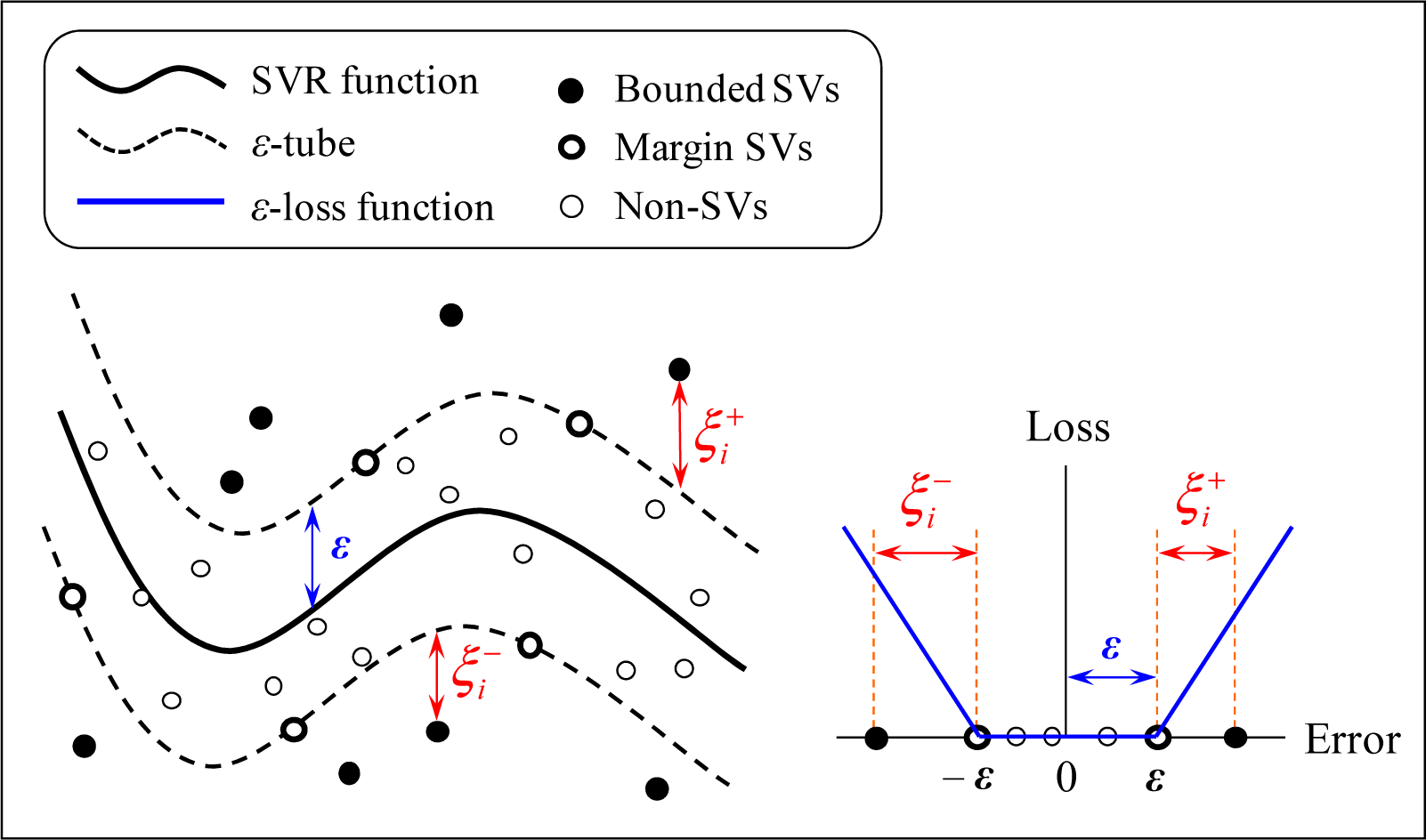
2.1. Support Vector Regression

SVR is a supervised learning method in which input and output data are assigned before learning begins. Let u be the input vector and v be the output variable. A regression function is constructed after u is mapped into a feature space by using a nonlinear function, Φ(u), as follows:
f ( x ) = w T Φ ( u ) + b
where vector w and variable b are parameters of the regression function. SVR differs from traditional regressions in the definition of the loss function. SVR uses Vapnik’s ε-insensitive loss function, Lτ, which penalizes only the data outside the ε-tube; the data within the extent of the ε-tube are tolerated and cause no loss. Figure 1 illustrates the mechanism of SVR and Vapnik’s ε-insensitive loss function, Lτ, which is formulated as follows:
L ε ( v i ) = { 0 for | v i [ w T Φ ( u i ) + b ] | < ε | v i [ w T Φ ( u i ) + b ] | ε , for | v i [ w T Φ ( u i ) + b ] | ε
where subscript i = 1, 2, …, l, and l is the number of data.
The SVR model can be formulated as the following optimization problem:
min w , b , ξ i + , ξ i 1 2 w T w + C i = 1 l ( ξ i + + ξ i ) subject to v i [ w T Φ ( u i ) + b ] ε + ξ i + [ w T Φ ( u i ) + b ] v i ε + ξ i ξ i + , ξ i 0 , i = 1 , 2 , , l
where ξ i + and ξ i are slack variables indicating the upper and lower training errors subject to error tolerance ε, and C is a positive cost constant that determines the level of penalized loss when a training error occurs (Figure 1). Using a dual set of Lagrange multipliers, α i + and α i , the optimization problem is solved by applying the standard quadratic programming algorithm.
max α + , α i = 1 l v i ( α i + α i ) ε i = 1 l ( α i + + α i ) 1 2 i , j = 1 l ( α i + α i ) ( α j + α j ) Φ ( u i ) T Φ ( u j ) subject to i = 1 l ( α i + α i ) = 0 0 α i + , α i C , i = 1 , 2 , l
The preceding objective function is a convex function, and the solution is unique and optimal. According to the solution provided by the Lagrange multipliers, α i + and α i , the parameters w and b in the SVR function can be calculated using complementarity conditions, where w = i = 1 l ( α i + α i ) Φ ( u i ). Therefore, the SVR function can be written as follows:
max α + , α i = 1 l v i ( α i + α i ) ε i = 1 l ( α i + + α i ) 1 2 i , j = 1 l ( α i + α i ) ( α j + α j ) Φ ( u i ) T Φ ( u j ) subject to i = 1 l ( α i + α i ) = 0 0 α i + , α i C , i = 1 , 2 , l
The inner products in this equation are computed using a kernel function, K ( u i , u ) = Φ ( u i ) T Φ ( u ). The Gaussian radial basis function with a parameter γ is used as the kernel:
K ( u i , u ) = exp ( γ | u i u | 2 )
In addition, let the Lagrange multiplier terms ( α i + α i ) be denoted as α ¯ i. Thus, the SVR function is written as follows:
f ( u ) = i = 1 l α ¯ i K ( u i , u ) + b
According to this equation, the data sets corresponding to zero coefficients α ¯ i are ineffective in the SVR function; only the data sets with nonzero coefficients α ¯ i are effective in the final SVR function. The data on the margin or outside the ε-insensitive tube have nonzero coefficients α ¯ i; therefore, these data are termed SVs that support the construction of the regression function. SVs with | α ¯ i | less than C are called margin SVs, and the SVs with | α ¯ i | equal to C are called bounded SVs. The margin SVs are located on the margin of the ε-tube, and the bounded SVs are outside the tube (Figure 1). Finally, the SVR function can be expressed as follows:
f ( u ) = s = 1 r α ¯ s K ( u s , u ) + b
where the subscript s represents the SV, and r is the number of SVs. The parameters of the SVR to be calibrated are the cost constant C, the error tolerance ε, and the kernel parameter γ. In this study, a two-step grid search method [11,55] was used to determine the parameters.

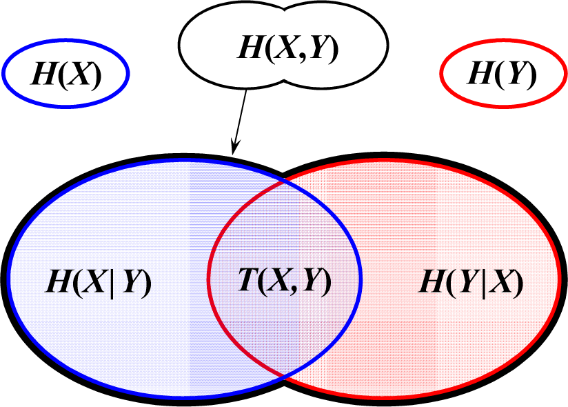
2.2. Information Entropy

Information entropy is used to quantify the amount of information in a data set. Shannon [30] introduced the concept of information entropy and mathematically formulated Shannon entropy H(X) for a discrete random variable X as follows:
H ( X ) = m = 1 M P ( x m ) log P ( x m )
where P(xm) is the probability of the outcome xm, and M is the number of outcomes. For continuous variables, such as the flood stages in this study, the entropy is calculated by dividing the domain of the variable into several class intervals. In this case, M is the number of class intervals. The entropy H(X) is nonnegative and its unit is typically expressed in bits when the base of the logarithm is 2. Entropy is a measure of the average amount of information or uncertainty contained in a random variable X. If the outcome of the variable is determinate, then it contains no uncertainty and, thus, no information (when this outcome is observed). In this certain case that the outcome is determinate, the entropy is 0.
The entropy H(X) for a single variable is also called the marginal entropy, in contrast to the joint entropy H(X,Y) of two variables:
H ( X , Y ) = m = 1 M n = 1 N P ( x m , y n ) log P ( x m , y n )
where P(xm,yn) is the joint probability of X=xm and Y=yn, and N is the number of class intervals of variable Y. For practical application, Markus et al. [43] and Mishra and Coulibaly [44] have set M equal to N; this setting was used in this study. The joint entropy represents the amount of combined information of the two variables. The joint entropy and marginal entropy are expressed in the formula as follows:
H ( X , Y ) = H ( X ) + H ( Y ) T ( X , Y )
where T(X,Y) is transinformation indicating the information that can be transferred from X to Y, or vice versa. Transinformation, also known as mutual information, is symmetrical so that T(X,Y) = T(Y,X). Transinformation is the partial information of one variable that can be obtained when a second variable is known. In other words, it is a measure of the shared information contained in one variable about a second variable. Figure 2 shows an information diagram illustrating the relationships among various entropies of two variables.
The conditional entropy H(X|Y) of X given Y is defined as follows:
H ( X | Y ) = m = 1 M n = 1 N P ( x m , y n ) log P ( x m | y n )
where P(xm|yn) is the conditional probability of X=xm given Y=yn. The conditional entropy H(X|Y) indicates the additional information required to quantify the marginal information of X when Y is known. Given the known transinformation T(X,Y), the conditional entropy H(X|Y) is the marginal information minus the transinformation:
H ( X | Y ) = H ( X ) T ( X , Y )
Similarly, the conditional entropy H(X|Y) is as follows:
H ( Y | X ) = H ( Y ) T ( X , Y )
Equations (13) and (14) show that less information exists in the conditional entropy than in the marginal entropy (Figure 2).
If X has a complete relationship with Y such that P(X|Y) =1, then H(X|Y) =0, and, thus, H(X)=T(X,Y). All information of X can be determined using transinformation if Y is known. If X and Y are independent, then H(X|Y)=H(X). This indicates that the transinformation is 0; the information of Y does not provide any information of X. Two variables are generally correlated, and the transinformation captures a specific quantity of the marginal information. The fraction of the amount of information of X that is obtained from Y can be evaluated according to R(X, Y) in Equation (15), which is the ratio of transinformation to marginal entropy. The transinformation ratio R(X, Y), ranging from zero to unity, is a relative measure of the dependence of X on Y. A similar concept of transinformation ratio was used in [42,43] as a measure of the information transmission in hydrometric network design.
R ( X , Y ) = T ( X , Y ) H ( X )

3. Mining Informative Hydrologic Data

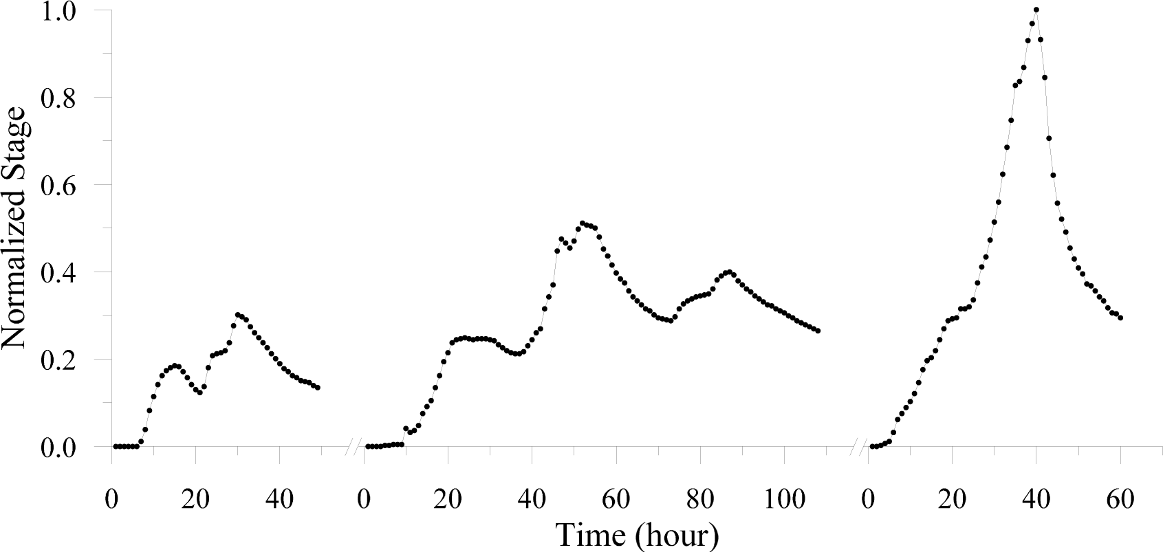
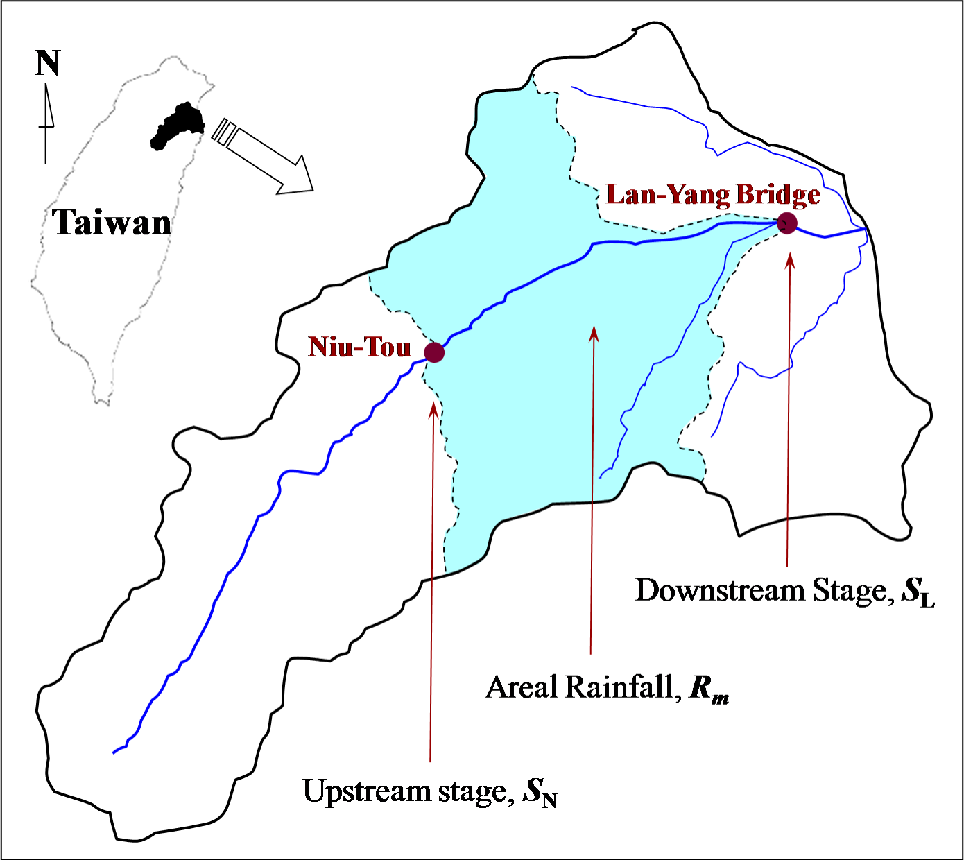
3.1. Hydrologic Data and Flood Forecasting Model

This study used the data and the SVR flood forecasting model developed in [13]. This section summarizes the hydrologic data used and the structure of the SVR flood forecasting model; a detailed description of the data and the model is provided in [13].
Hourly hydrologic data, namely flood stage and rainfall data in the Lan-Yang River basin in Taiwan, were used. The flood stage data were from two water level stations, the downstream Lan-Yang Bridge Station and upstream Niu-Tou Station, and the rainfall data were records of the areal rainfall accumulated in the catchment area between Lan-Yang Bridge and Niu-Tou Stations. Figure 3 presents the map of Lan-Yang River basin and the location of stations. The distance between the upstream and downstream stations is approximately 25 km. Complete records of flood stage and rainfall data measuring flood events were obtained, and 12 flood events from 1990 to 2001 were used for model development.
The output variable of the flood forecasting model was the downstream flood stage at the Lan-Yang Bridge at time t, denoted as SL(t). The input variables were the flood stage at the Lan-Yang Bridge at time t − 1, denoted as SL(t − 1); the upstream stage at Niu-Tou at time t − 3, denoted as SN(t − 3); and the average of the areal rainfall at times t − 1 to t − 5, denoted as Rm(t − 5). The above time lags of the input variables were determined on the basis of the hydrologic response time [11,13,57,58]. The lag for upstream stage SN was determined by calculating the coefficient of correlation with different time lags between the upstream and downstream stage series, and by identifying the time lags of significant feature points, such as the peak stage, of the stage hydrographs with respect to each flood event. Based on the methods, the average time lag for SN is 3.3 h. The lag of rainfall Rm was determined by using the time of concentration according to the same concept of hydrologic response time. The average time of concentration pertaining to flood events is 5.3 h. The lagged input variables that are most relevant to the output variable are used in the model. Therefore, the SVR flood forecasting model can be expressed as follows:
S L ( t ) = f SVR [ S L ( t 1 ) , R m ( t 5 ) , S N ( t 3 ) ]
where fSVR represents the SVR model.
According to the model structure with lagged variables, 963 input-output data sets were available for analysis. The variables of the model were normalized to the interval from 0 to 1, according to the minimum and maximum data. This method is commonly adopted in data-driven models to prevent the model from being dominated by variables with high values. The following discussion on the hydrologic data and the calculated information indices are based on the normalized hydrologic data, of which the values are between 0 and 1. In the constructed SVR model in [13], 63% of the data were SVs. SVs were pruned in [13], and the remaining SVs were informative hydrologic data characterizing the flood process.

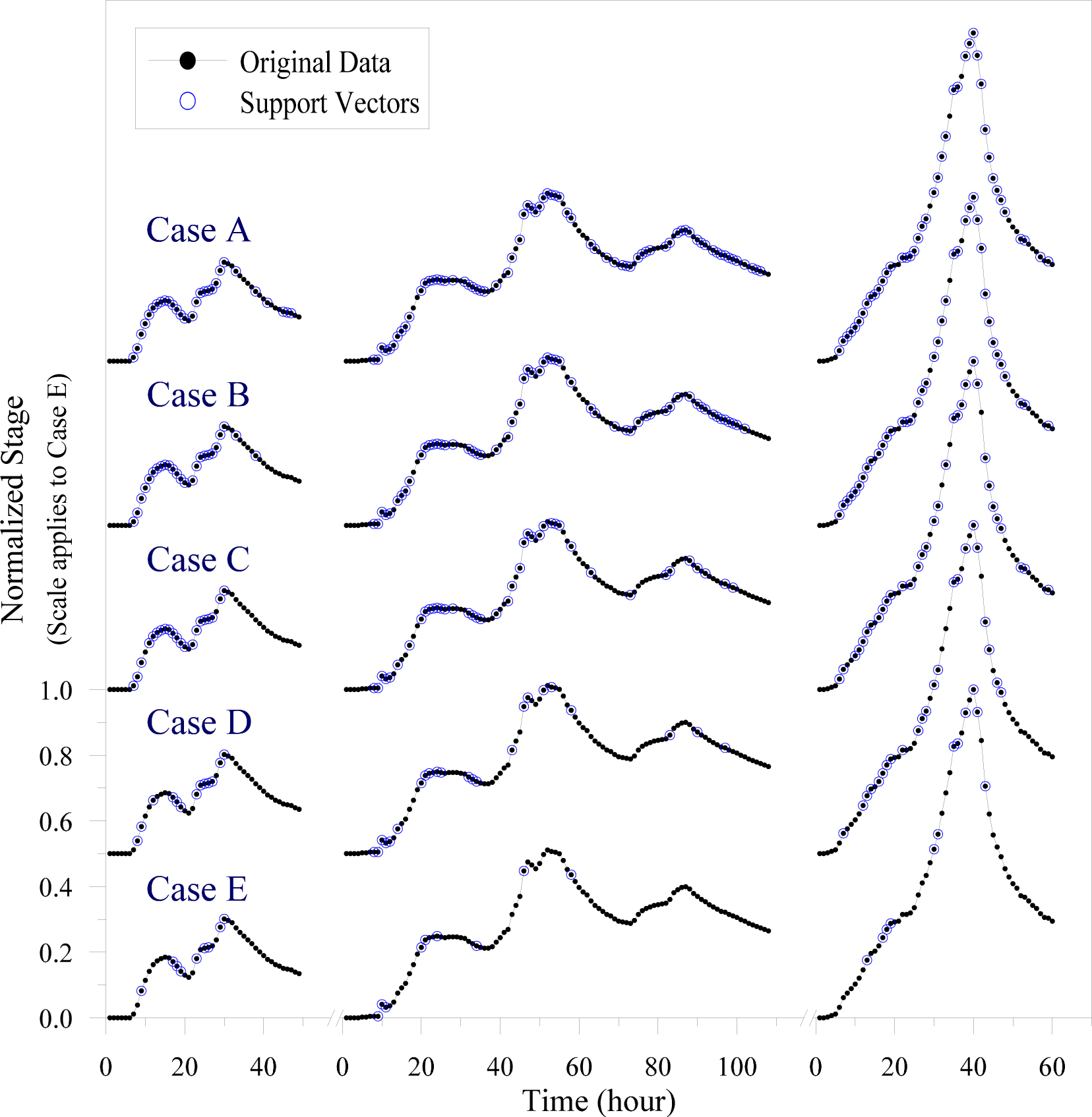
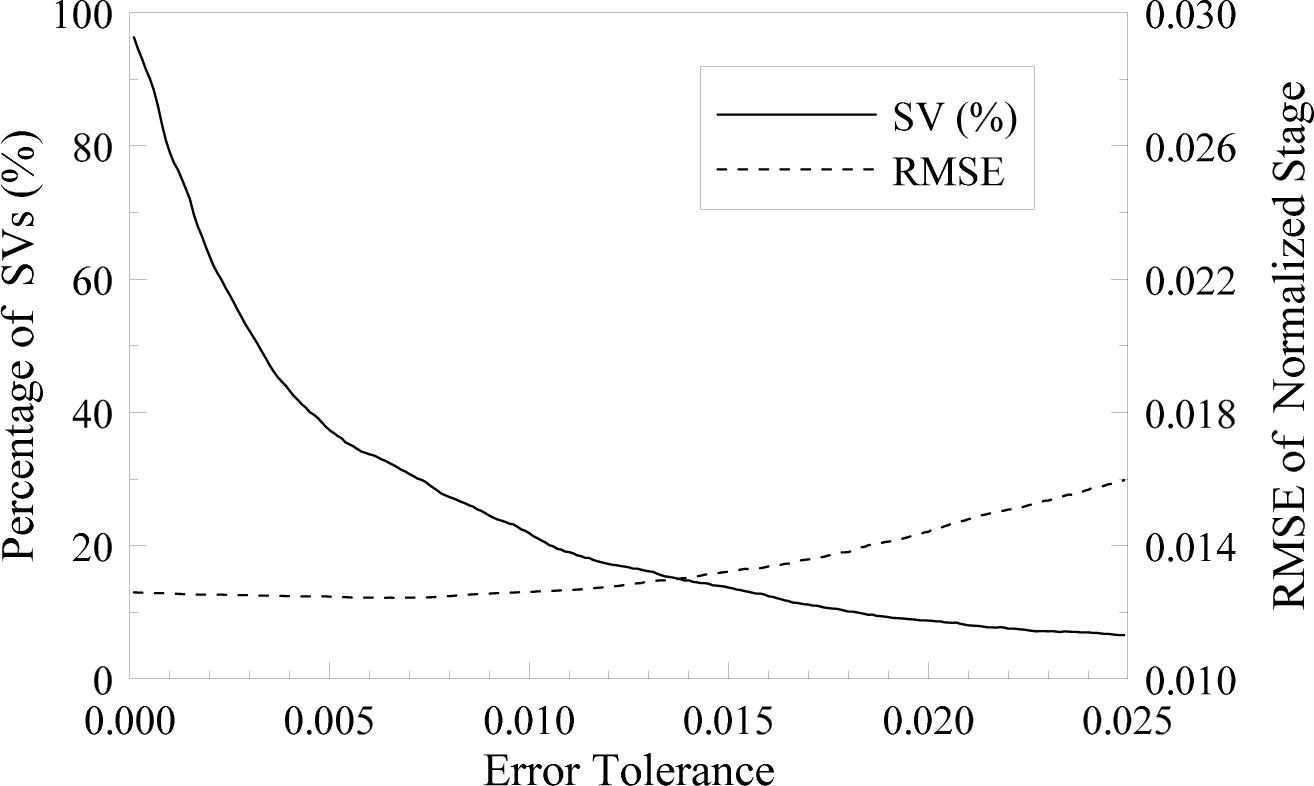
3.2. Support Vectors as Informative Data

Chen and Yu [13] demonstrated that SVs are types of informative flood data and suggested that the SV pruning method is a data mining technique for extracting condensed informative hydrologic data. The pruning method is based on a strong relationship between the error tolerance ε and the number of SVs. Considering several fixed sets of cost constant C and the kernel parameter γ values, with different ε values used to build the SVR models, the correlation between ε and the percentage of SVs can be obtained. Figure 4 shows the relationship between ε values and the percentages of SVs from the analysis performed in [13], which depicts the detailed process to derive the relationship. The current study used this relationship to control the number of SVs by setting appropriate ε values. It investigated five data mining cases to extract 50%, 40%, 30%, 20%, and 10% of the flood data (denoted as Cases A to E, respectively). Five SVR models were calibrated by constraining the ε value within a small interval corresponding to the desired percentage of SVs according to Figure 4. The two-step grid search method [11,55] was then used to determine the parameters of the SVR models, although the parameter ε was kept in a small interval that was in line with the desired percentage of SVs. The parameter search was conducted by using a coarse grid and a finer grid to find the optimal parameters. A six-fold cross-validation was employed in this study. Table 1 presents the calibrated parameters and data mining results of the SVs. The parameter and root mean square error (RMSE) values were similar to those in [13], and the values of mined SVs were approximately the desired percentages of 50%, 40%, 30%, 20%, and 10% (from a total of 963 data sets).
To demonstrate the mining results, Figure 5 shows three flood events of typical small, medium, and large sizes on a scale of normalized flood stages. Figure 6 illustrates the process of pruning SVs from 50% to 10% (Cases A to E), and shows that informative flood data, particularly the data around the peak stage and in the rising limb, were typically mined as SVs. The results of the data mining process are described as follows [13]: (1) data around the peak stage were mined as SVs; (2) a majority of data in the rising limb of the hydrograph remained SVs; and (3) data in the recession limb were eliminated during the data mining process. These results prove that informative data that characterized the flood hydrograph were mined as SVs, and that SVs obtained using the proposed SVR model represent informative hydrologic data. Moreover, the SVR flood forecasting models constructed using fewer SVs performed equally well in providing real-time flood forecasting as those constructed with more SVs did [13], indicating that the pruned SVs contained sufficient information to describe the flood process. The SVs mined using the SVR method were hydrologically interpreted as informative data, and the following section describes the use of entropy indices to quantify the amount of information in the mined informative hydrologic data.

4. Assessment of Information Entropy

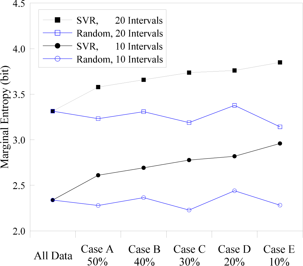
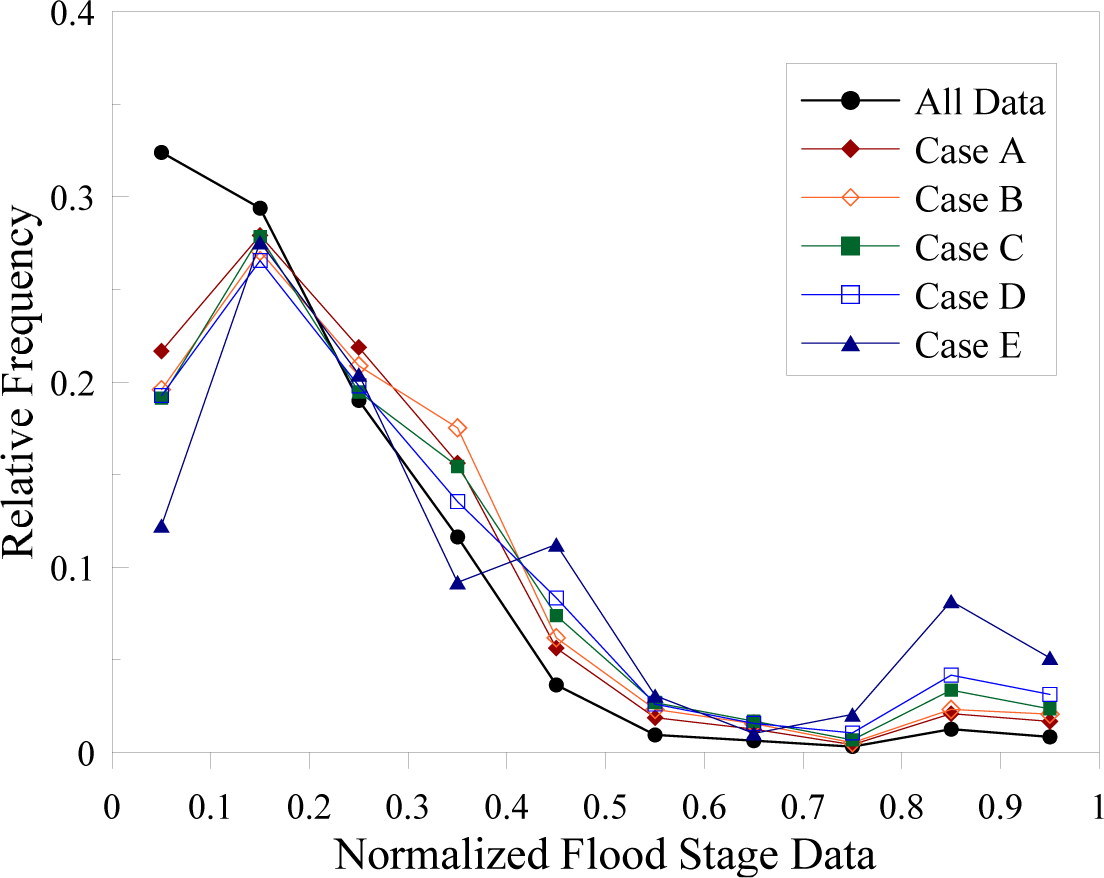
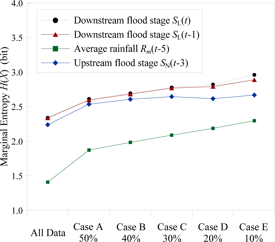
4.1. Marginal Entropies of the Flood Stages and Support Vectors

Entropy measures the amount of information contained in a data set. To calculate the marginal entropy of a data set by using Equation (9), the number of class intervals of the data must be specified. The number of class intervals can influence the value of entropy, but the relative amount of information is not sensitive to the number of intervals, as stated in [43,44]. This study used 10 and 20 intervals to test the influence of the number of intervals on entropy. It also compared the entropy indices related to the mined SVs and the randomly selected data of the output flood stage variable SL(t). Figure 7 shows the marginal entropies of all flood stage data, as well as the SVs of Cases A to E for 10 and 20 class intervals. The marginal entropies for the 20 intervals were greater than those for the 10 intervals, indicating that data categorized into more intervals contained more information. The results in Figure 7 confirm that the number of intervals influenced entropy values, but did not alter the relative pattern of information indices. In the following analysis and interpretation of various entropy indices, 10 class intervals of data were used because the relative information measures were not sensitive to the number of intervals, and using 20 intervals would result in numerous empty intervals when calculating entropies for two variables.
Figure 7 also shows that the entropies of mined data increased as the number of SVs decreased, but the entropies of the randomly selected 50% to 10% of the data (the same number as those of the SVs in Cases A to E) were comparable. This phenomenon can be explained in terms of data compression; compressed data contain less redundancy and have higher entropy. If a data set contains an excessive amount of unnecessary information, then it is more redundant and less informative. Therefore, the higher the entropy, the more informative and less redundant a data set is. Redundant flood data in the mined SV data sets were pruned, causing the data sets to become compressed and more informative. Therefore, the mined SVs were more compact and had higher entropy. The randomly selected data sets had similar characteristics (redundancy or information) as the original data set did; therefore, the entropies were comparable. Accordingly, the SVs mined using the SVR method were determined to be meaningful and informative hydrologic data based on entropy theory.
Figure 8 shows the relative frequencies related to various class intervals of the normalized flood stage data. In the data mining process from Cases A to E, the percentages of low stage data decreased and the percentages of high stage data increased. The relative frequency curves in Figure 8 provide additional information on the percentages of mined SVs, and confirm that higher flood stages are mined as SVs and lower flood stages tend to be pruned.

4.2. Entropies Related to Various Hydrologic Variables

The flood forecasting model contains one output and three input variables: the output downstream flood stage SL(t); the input downstream flood stage SL(t − 1); the input average rainfall Rm(t − 5), and the input upstream flood stage SN(t − 3). The various entropy indices relating to these four variables were calculated and listed in Tables 2 and 4 (each table relates the output variable to an input variable).
Figure 9 shows the marginal entropies of all and mined data regarding the four variables. The marginal entropy is a measure of the average amount of information contained in a hydrologic variable. The marginal entropies of the four variables increased as the number of mined data decreased, indicating that the SVR method mined informative hydrologic data regarding these variables. Two downstream stage variables (with a lag of 1 h) showed similar entropies. The output variable SL(t) had a slightly higher entropy than the input variable SL(t − 1) did, suggesting that the SVR model mined the SVs by forecasting the output variable; therefore, the output variable showed a slightly higher entropy. This also explains the entropies regarding the output downstream stage SL(t) and input upstream stage SN(t − 3); the entropies of SL(t) were higher than those of SN(t − 3) were. The marginal entropies of the rainfall variable Rm(t − 5) were lower than those of the stage variables. Regarding the hydrologic process, rainfall provided indirect and less concrete information on a flood event than the stage did. Therefore, the flood stage was a more informative hydrologic variable than rainfall.
Figure 10 shows the joint entropies of all and mined data regarding the output variable and three respective input variables. The joint entropy measures the combined information of two variables. Figure 10 shows that the joint entropies generally increased as the amount of mined data decreased. The joint entropies of SL(t) and SL(t − 1) were the lowest because these two variables contained similar types of information. However, the joint entropies of SL(t) and SL(t − 1) were higher than the marginal entropy of SL(t), indicating that the pair of successive flood stages provided more information on the floods than only one flood stage did. The joint entropies of SL(t) and SN(t − 3) were higher than those of SL(t) and Rm(t − 5), although they were close with respect to 20% and 10% of the data. The results of joint entropies in Figure 10 show that a Muskingum-type river routing model constructed using the downstream and upstream stage variables, SL(t) and SN(t − 3), may be more effective than a rainfall-runoff (or rainfall-stage) model constructed using the rainfall and downstream stage variables, Rm(t − 5) and SL(t), in terms of the total information used to describe the hydrologic process. Moreover, these two hydrologic models may outperform an autoregressive model constructed using SL(t) and SL(t − 1).
Transinformation is a measure of the common information shared by two variables. The partial information of SL(t) that can be known from a second variable can be assessed according to the ratio of transinformation to marginal entropy by using Equation (15). Therefore, transinformation can be considered a measure of dependence of one variable on another. Figure 11 shows the transinformation ratios R(X, Y) of all and mined data regarding the output flood stage SL(t) and three respective input variables. The transinformation ratios of R[SL(t), SL(t − 1)] ranged from 0.64 to 0.79 (cf. Table 2), meaning that approximately 65% to 80% of the information on SL(t) could be known from SL(t − 1). The transinformation ratios of R[SL(t), SN(t − 3)] were approximately 30%, and those of R[SL(t), Rm(t − 5)] were approximately 10% to 20%. The upstream stage variable SN(t − 3) contained more mutual information with SL(t) than did the rainfall variable Rm(t − 5). An interesting issue regarding transinformation in Figure 11 is that the lines in the figure show different trends. The increases in the variables SN(t − 3) and Rm(t − 5) as the number of SVs decreased indicated that the mined informative data showed a stronger relationship (or dependence) between the two variables and SL(t). However, the decrease in the variable SL(t − 1) as the number of SVs decreased cannot be explained according to this interpretation. SL(t) and SL(t − 1) were the same variable with a 1-hour lag. They shared more mutual information when the amount of data was increased. When the amount of data was reduced (even though the data were more informative to characterized a flood hydrograph), the dependence between SL(t) and SL(t − 1) was reduced.
The results shown in Figure 11 confirm the hydrologic modeling and forecasting concept of Equation (16), which provides the output of SL(t) and three inputs of SL(t − 1), Rm(t − 5), and SN(t − 3). With this input-output structure of the model, the dominating input variable was determined to be SL(t − 1), which was the lagged variable of the output. The upstream flood stage SN(t − 3) had secondary importance to the output of the downstream flood stage. Rainfall was a supplement used to adjust the modeling or forecasting and had the lowest level of direct influence on the output. The results of the transinformation ratio in Figure 11 verify the aforementioned concept of hydrologic modeling that was obtained through sensitivity analysis.

5. Conclusions

This study adopted SVR as a method for mining informative hydrologic data. Flood stage and rainfall data in the Lan-Yang River basin in Taiwan and the SVR model developed in [13] were used for the case study. Data mining results demonstrated that the mined data were informative hydrologic data that characterized a flood hydrograph.
Furthermore, this study applied entropy theory to quantify the mined hydrologic data and verified that the mined data showed a meaningful hydrologic interpretation by using entropy indices. The mined flood stage data, of which the percentage was reduced from 50% to 10%, had increased entropies, indicating that the mined data were more informative than the original data. Marginal entropies regarding various input and output variables showed that the flood stage was a more informative hydrologic variable than rainfall because rainfall provided less direct information on a flood event than the flood stage did. Analysis results of joint entropies implied that a hydrologic model with variables containing more total information was superior to a model containing variables with less total information. Transinformation was used to quantify the mutual information of two hydrologic variables and explained the relative importance of the input stage and rainfall variables on the output stage variable.
This study successfully used entropy theory to meaningfully explain the information contained in mined hydrologic data. Future research on the interpretation of various hydrologic processes by using entropy theory is necessary. Related topics that were not discussed in this study, but are subjects worthy of further research, include the relationship between entropy indices and model performance, and using entropy indices as the objective function to maximize model forecasting accuracy.

Conflicts of Interest

The author declares no conflict of interest.

References

  1. Vapnik, V.N. The Nature of Statistical Learning Theory; Springer-Verlag: New York, NY, USA, 1995. [Google Scholar]
  2. Vapnik, V.N. Statistical Learning Theory; Wiley: New York, NY, USA, 1998. [Google Scholar]
  3. Yu, X.; Liong, S.Y.; Babovic, V. EC-SVM approach for real-time hydrologic forecasting. J. Hydroinform. 2004, 6, 209–223. [Google Scholar]
  4. Bray, M.; Han, D. Identification of support vector machines for runoff modeling. J. Hydroinform. 2004, 6, 265–280. [Google Scholar]
  5. Sivapragasam, C.; Liong, S.Y. Flow categorization model for improving forecasting. Nord. Hydrol. 2005, 36, 37–48. [Google Scholar]
  6. Han, D.; Chan, L.; Zhu, N. Flood forecasting using support vector machines. J. Hydroinform. 2007, 9, 267–276. [Google Scholar]
  7. Lin, G.F.; Chen, G.R.; Huang, P.Y.; Chou, Y.C. Support vector machine-based models for hourly reservoir inflow forecasting during typhoon-warning periods. J. Hydrol. 2009, 372, 17–29. [Google Scholar]
  8. Lin, G.F.; Chou, Y.C.; Wu, M.C. Typhoon flood forecasting using integrated two-stage support vector machine approach. J. Hydrol. 2013, 486, 334–342. [Google Scholar]
  9. Wu, M.C.; Lin, G.F.; Lin, H.Y. Improving the forecasts of extreme streamflow by support vector regression with the data extracted by self-organizing map. Hydrol. Process. 2014, 28, 386–397. [Google Scholar]
  10. Liong, S.Y.; Sivapragasam, C. Flood stage forecasting with support vector machines. J. Am. Water Resour. Assoc. 2002, 38, 173–196. [Google Scholar]
  11. Yu, P.S.; Chen, S.T.; Chang, I.F. Support vector regression for real-time flood stage forecasting. J. Hydrol. 2006, 328, 704–716. [Google Scholar]
  12. Chen, S.T.; Yu, P.S. Real-time probabilistic forecasting of flood stages. J. Hydrol. 2007, 340, 63–77. [Google Scholar]
  13. Chen, S.T.; Yu, P.S. Pruning of support vector networks on flood forecasting. J. Hydrol. 2007, 347, 67–78. [Google Scholar]
  14. Aggarwal, S.K.; Goel, A.; Singh, V.P. Stage and discharge forecasting by SVM and ANN Techniques. Water Resour. Manag. 2012, 26, 3705–3724. [Google Scholar]
  15. Wei, C.C. Wavelet kernel support vector machines forecasting techniques: Case study on water-level predictions during typhoons. Expert Syst. Appl. 2012, 39, 5189–5199. [Google Scholar]
  16. Sivapragasam, C.; Liong, S.Y.; Pasha, M.F.K. Rainfall and runoff forecasting with SSA-SVM approach. J. Hydroinform. 2001, 3, 141–152. [Google Scholar]
  17. Sumi, S.M.; Zaman, M.F.; Hirose, H. A rainfall forecasting method using machine learning models and its application to the Fukuoka City case. Int. J. Appl. Math. Comput. Sci. 2012, 22, 841–854. [Google Scholar]
  18. Nikam, V.; Gupta, K. SVM-based model for short-term rainfall forecasts at a local scale in the Mumbai urban area, India. J. Hydrol. Eng. 2014, 19, 1048–1052. [Google Scholar]
  19. Chen, S.T. Multiclass support vector classification to estimate typhoon rainfall distribution. Disaster Adv. 2013, 6, 110–121. [Google Scholar]
  20. Lin, G.F.; Jhong, B.C.; Chang, C.C. Development of an effective data-driven model for hourly typhoon rainfall forecasting. J. Hydrol. 2013, 495, 52–63. [Google Scholar]
  21. Lin, G.F.; Jhong, B.C. A real-time forecasting model for the spatial distribution of typhoon rainfall. J. Hydrol. 2015, 521, 302–313. [Google Scholar]
  22. Chen, S.T.; Yu, P.S.; Liu, B.W. Comparison of neural network architectures and inputs for radar rainfall adjustment for typhoon events. J. Hydrol. 2011, 405, 150–160. [Google Scholar]
  23. Kusiak, A.; Wei, X.P.; Verma, A.P.; Roz, E. Modeling and prediction of rainfall using radar reflectivity data: A data-mining approach. IEEE Trans. Geosci. Remote Sens. 2013, 51, 2337–2342. [Google Scholar]
  24. Tripathi, S.; Srinivas, V.V.; Nanjundiah, R.S. Downscaling of precipitation for climate change scenarios: A support vector machine approach. J. Hydrol. 2006, 330, 621–640. [Google Scholar]
  25. Kaheil, Y.H.; Rosero, E.; Gill, M.K.; Mckee, M.; Bastidas, L.A. Downscaling and forecasting of evapotranspiration using a synthetic model of wavelets and support vector machines. IEEE Trans. Geosci. Remote Sens. 2008, 46, 2692–2707. [Google Scholar]
  26. Chen, S.T.; Yu, P.S.; Tang, Y.H. Statistical downscaling of daily precipitation using support vector machines and multivariate analysis. J. Hydrol. 2010, 385, 13–22. [Google Scholar]
  27. Yang, T.C.; Yu, P.S.; Wei, C.M.; Chen, S.T. Projection of climate change for daily precipitation: A case study in Shih-Men Reservoir catchment in Taiwan. Hydrol. Process. 2011, 25, 1342–1354. [Google Scholar]
  28. Mao, K.Z. Feature subset selection for support vector machines through discriminative function pruning analysis. IEEE Trans. Syst. Man Cybern. B 2004, 34, 60–67. [Google Scholar]
  29. Hao, P.Y.; Chiang, J.H. Pruning and model-selecting algorithms in the RBF frameworks constructed by support vector learning. Int. J. Neural Syst. 2006, 16, 283–293. [Google Scholar]
  30. Shannon, C.E. A mathematical theory of communication. Bell Syst. Tech. J. 1948, 27. [Google Scholar]
  31. Sonuga, J.O. Principle of maximum entropy in hydrologic frequency analysis. J. Hydrol. 1972, 17, 177–191. [Google Scholar]
  32. Jowitt, P.W. The extreme-value type-1 distribution and the principle of maximum entropy. J. Hydrol. 1979, 42, 23–38. [Google Scholar]
  33. Padmanabhan, G.; Rao, A.R. Maximum entropy spectral analysis of hydrologic data. Water Resour. Res. 1988, 24, 1519–1533. [Google Scholar]
  34. Yu, H.L.; Chen, J.C.; Christakos, G. BME Estimation of Residential Exposure to Ambient PM10 and Ozone at Multiple Time-Scales. Environ. Health Perspect. 2009, 117, 537–544. [Google Scholar]
  35. Yu, H.L.; Chu, H.J. Understanding Space-time Patterns of Groundwater Systems by Empirical Orthogonal Functions: A case study in the Choshui River Alluvial Fan, Taiwan. J. Hydrol. 2010, 381, 239–247. [Google Scholar]
  36. Yu, H.L.; Wang, C.H.; Liu, M.C.; Kuo, Y.M. Estimation of fine particulate matter in Taipei using landuse regression and Bayesian maximum entropy methods. Int. J. Environ. Res. Public Health. 2011, 8, 2153–2169. [Google Scholar]
  37. Yu, H.L.; Wang, C.H. Quantile-based Bayesian maximum entropy approach for spatiotemporal modeling of ambient air quality levels. Environ. Sci. Technol. 2013, 47, 1416–1424. [Google Scholar]
  38. Amorocho, J.; Espildora, B. Entropy in the assessment of uncertainty in hydrologic systems and models. Water Resour. Res. 1973, 9, 1511–1522. [Google Scholar]
  39. Chapman, T.G. Entropy as a measure of hydrologic data uncertainty and model performance. J. Hydrol. 1986, 85, 111–126. [Google Scholar]
  40. Husain, T. Hydrologic uncertainty measure and network design. Water Resour. Bull. 1989, 25, 527–534. [Google Scholar]
  41. Harmancioglu, N.B.; Alpaslan, N. Water quality monitoring network design: A problem of multi-objective decision making. AWRA Water Resour. Bull. 1992, 28, 179–192. [Google Scholar]
  42. Yang, Y.; Burn, D.H. An entropy approach to data collection network design. J. Hydrol. 1994, 157, 307–324. [Google Scholar]
  43. Markus, M.; Knapp, H.V.; Tasker, G.D. Entropy and generalized least square methods in assessment of the regional value of streamgages. J. Hydrol. 2003, 283, 107–121. [Google Scholar]
  44. Mishra, A.K.; Coulibaly, P. Hydrometric network evaluation for Canadian watersheds. J. Hydrol. 2010, 380, 420–437. [Google Scholar]
  45. Chen, Y.C.; Kuo, J.J.; Yu, S.R.; Liao, Y.J.; Yang, H.C. Discharge estimation in a lined canal using information entropy. Entropy 2014, 16, 1728–1742. [Google Scholar]
  46. Wei, C.; Yeh, H.C.; Chen, Y.C. Spatiotemporal scaling effect on rainfall network design using entropy. Entropy 2014, 16, 4626–4647. [Google Scholar]
  47. Singh, V.P. The use of entropy in hydrology and water resources. Hydrol. Process. 1997, 11, 587–626. [Google Scholar]
  48. Mishra, A.K.; Coulibaly, P. Development in hydrometric networks design: A review. Rev. Geophys. 2009, 47. [Google Scholar] [CrossRef]
  49. Sang, Y.F.; Wang, D.; Wu, J.C.; Zhu, Q.P.; Wang, L. Wavelet-based analysis on the complexity of hydrologic series data under multi-temporal scales. Entropy 2011, 13, 195–210. [Google Scholar]
  50. Zhang, L.; Singh, V.P. Bivariate rainfall and runoff analysis using entropy and copula theories. Entropy 2012, 14, 1784–1812. [Google Scholar]
  51. Ahmadi, A.; Han, D.; Karamouz, M.; Remesan, R. Input data selection for solar radiation estimation. Hydrol. Process. 2009, 23, 2754–2764. [Google Scholar]
  52. Remesan, R.; Azadeh, A.; Muhammad Ali, S.; Han, D. Effect of data time interval on real-time flood forecasting. J. Hydroinform. 2010, 12, 396–407. [Google Scholar]
  53. Ahmadi, A.; Han, D.; Lafdani, E.K.; Moridi, A. Input selection for long-lead precipitation prediction using large-scale climate variables: A case study. J. Hydroinform. 2015, 17, 114–129. [Google Scholar]
  54. Singh, V.P. Hydrologic synthesis using entropy theory: Review. J. Hydrol. Eng. 2011, 16, 421–433. [Google Scholar]
  55. Hsu, C.W.; Chang, C.C.; Lin, C.J. A Practical Guide to Support Vector Classification. Available online: http://www.csie.ntu.edu.tw/~cjlin/papers/guide/guide.pdf accessed on 16 December 2014.
  56. Wikipedia: Joint entropy. Available online: http://en.wikipedia.org/wiki/Joint_entropy accessed on 16 December 2014.
  57. Solomatine, D.P.; Dulal, K.N. Model trees as an alternative to neural networks in rainfall-runoff modelling. Hydrol. Sci. J. 2003, 48, 399–411. [Google Scholar]
  58. Chen, C.S.; Jhong, Y.D.; Wu, T.Y.; Chen, S.T. Typhoon event-based evolutionary fuzzy inference model for flood stage forecasting. J. Hydrol. 2013, 490, 134–143. [Google Scholar]
Figure 1. Illustration of SVR (modified from [11]).
Entropy 17 01023f1
Figure 2. Information diagram illustrating the relationships among the marginal entropies H(X) and H(Y), joint entropy H(X, Y), transinformation T(X, Y), and conditional entropies H(X | Y) and H(Y | X) (modified from [56]).
Entropy 17 01023f2
Figure 3. Location of stations with hydrologic variables.
Entropy 17 01023f3
Figure 4. Relationship between error tolerance ε and the percentages of SVs, as well as between ε and the RMSE in [13].
Entropy 17 01023f4
Figure 5. Small, medium, and large flood events used to demonstrate the mining of informative hydrologic data.
Entropy 17 01023f5
Figure 6. Process of pruning SVs to mine informative hydrologic data.
Entropy 17 01023f6
Figure 7. Marginal entropies for various data sets and intervals.
Entropy 17 01023f7
Figure 8. Relative frequencies relating to various class intervals of flood stage data.
Entropy 17 01023f8
Figure 9. Marginal entropies of all and mined data regarding four variables.
Entropy 17 01023f9
Figure 10. Joint entropies of all and mined data regarding the output downstream flood stage SL(t) and three respective input variables.
Entropy 17 01023f10
Figure 11. Transinformation ratios of all and mined data regarding the output downstream flood stage SL(t) and three respective input variables.
Entropy 17 01023f11
Table 1. Calibrated parameters and results of SVs.
CaseParameters
Number of SVsPercentage of SVs (%)RMSE
Cεγ
Case A40.80.00320.13148049.80.0127
Case B47.30.00450.13438840.30.0126
Case C54.30.00720.16429830.90.0124
Case D50.30.01050.17319219.90.0126
Case E49.00.01820.1839810.20.0139
Table 2. Entropies relating to variables of the output downstream flood stage X = SL(t) and the input downstream flood stage Y = SL(t − 1).
EntropyAll DataCase ACase BCase CCase DCase E
H(X)2.342.612.692.782.822.96
H(X|Y)0.490.680.760.820.911.06
T(X,Y)1.851.931.931.961.911.90
H(Y|X)0.490.660.750.810.880.98
H(Y)2.342.592.682.772.792.89
H(X,Y)2.833.273.443.593.703.94
R(X,Y)0.790.740.720.700.680.64
Table 3. Entropies relating to variables of the output downstream flood stage X = SL(t) and the input average rainfall Y = Rm(t − 5).
EntropyAll DataCase ACase BCase CCase DCase E
H(X)2.342.612.692.782.822.96
H(X|Y)2.122.352.412.422.372.28
T(X,Y)0.220.270.290.360.450.68
H(Y|X)1.191.601.701.731.741.62
H(Y)1.411.871.982.092.182.30
H(X,Y)3.534.224.394.514.564.57
R(X,Y)0.090.100.110.130.160.23
Table 4. Entropies relating to variables of the output downstream flood stage X = SL(t) and the input upstream flood stage Y = SN(t − 3).
EntropyAll DataCase ACase BCase CCase DCase E
H(X)2.342.612.692.782.822.96
H(X|Y)1.651.921.982.032.001.96
T(X,Y)0.690.690.710.750.821.00
H(Y|X)1.551.841.891.901.801.66
H(Y)2.242.532.612.642.612.67
H(X,Y)3.884.464.594.684.624.62
R(X,Y)0.300.260.260.270.290.34

