EWnFM: An Environment States Oriented Web Service Non-Functional Property Model

Abstract

A proper model of Web service non-functional properties is the key foundation to the evaluation of non-functional properties of Adaptive Service Based Software (ASBS) systems. As the environment in which a Web service is deployed may keep changing, environmental factors would affect the non-functional properties of a Web service a lot. However, available non-functional property models usually ignore the impact of environmental factors, leading to insufficient modeling power of non-functional properties, limited effect of system wide non-functional property evaluation based on these models, and the inability to support environment states oriented specifications of ASBS. This paper propose an environment states oriented Web service non-functional property model. By considering the differences of a non-functional property under different environment states, environment states of a Web service is analyzed using a Dirichlet process based method. With such a foundation, an environment states oriented Web service non-functional property model is introduced, together with the parameter estimation methods based on historical monitor data. Experiment results have shown that compared to the evaluated methods, our model could generate data that are much close to real monitored data.

1. Introduction

Taking the advantage of loose coupling and delayed binding, Service Based Software (SBS) systems implement Service-Oriented Architecture (SOA)-based large scale distributed applications by rapid composition of Web services. Meanwhile, according to predefined adaptation strategies, Adaptive SBS (ASBS) dynamically self adjust to changing execution situations, allowing systems to complete business functions while assuring non-functional properties [1] by adaptive adjusting with minimized manual interventions. As an important way to improve SBS quality in open and dynamic environments, ASBS have received lots of attention from the field of network-distributed software systems research.

The construction of SBS focuses on business logic design and Web service selection, with no need to develop or deploy Web service instances. Web services published and deployed in open network environments by service providers are, in essence, autonomous. Since SBS are unable to guarantee the quality of these services, system evaluation during the design phase of SBS construction is important for quality assurance of SBS [2,3]. ASBS extend SBS by enabling strategy-based adaptation. By instructing SBS to self-adjust to changing execution situations using predefined adaptation strategies, ASBS improve the quality of the systems. To this end, ASBS adaptation strategy evaluation is a key issue to be resolved in ASBS research. Since non-functional properties of SBS, such as response time, are the key considerations in the construction of SBS, analyzing the impacts that the adaptation strategies of ASBS have on non-functional properties is one of the most important works for ASBS adaptation strategy evaluation. To achieve this goal, the most fundamental prerequisite is to present models of non-functional properties.

To model non-functional properties of Web services, UML profile for Schedulability, Performance and Time (UML-SPT) [4], which is widely used in software engineering, is adapted in most service composition studies [5–7]. Web service oriented description languages such as Performance-enable Web Service Definition Language (P-WSDL) [8] and Kernel Language for Performance and Reliability (KLAPER) analysis [9] etc. are also introduced. Labels corresponding to non-functional properties of Web services are defined in these languages. Detailed descriptions are then given by domain experts in the form of mean values or probabilistic models based on previous experiences. Mean values are widely used in performance analysis due to their product property [10]. On the other hand, probabilistic models describe the distributions of non-functional properties, and thus more details could be captured than using simple mean values. For example, most current studies use exponential distributions to describe the response time of Web services [4,7,8].

As Web services are deployed on Internet servers, execution of Web services could be significantly affected by environment factors. For example, when a host server is overloaded, Web service processes could be kept stalled in waiting states, leading to drops in execution efficiency, response time and service availability. In this case, performance of non-functional properties such as response time shows great differences with those on idle servers. Therefore, when analyzing non-functional properties of Web services, if we focus solely on the properties themselves but with environmental impacts ignored, it would be difficult to finely present models for non-functional properties.

In order to consider environmental impacts on non-functional properties, state-associated probabilistic models such as Markov Arrival Process (MAP) and Markov Modulated Poisson Process (MMPP) have been applied to non-functional property modeling in recent years. For example, for frequently seen unexpected situations in network applications such as workload bursty and flash-crowd [11,12] analyzed the shortages of handling burst requests using traditional modeling and evaluation approaches in Multi-tier Application systems, and proposed a modeling approach based on MAP for response time. In [13], the work of [12] was extended for similar situations by proposing a modeling approach for service load based on MMPP. The key idea of these works is to analyze the differences in the performance of non-functional properties under different states based on historical data of non-functional properties and some predefined environment states (e.g., bursty and normal), whereby introducing non-functional property models related to these environment states. Compared with the traditional approaches, studies considering environment states could provide more detailed models for response time, server load and other non-functional properties. However, disadvantages in the processing of environment states still affect the application of these approaches.

Firstly, for models based on MAP and MMPP, a key prerequisite is to predefine possible environment states. For example, in [12] and [13], two environment states, bursty and normal, are considered. Generally speaking, environmental factors that may affect non-functional properties are numerous, and the impacts of these factors on a specific non-functional property is very complicated. Since environment states comprehensively reflect the impact factors of non-functional properties and the interactions between these factors, it would be improper to predefine environment states solely based on burstiness. Furthermore, considering the complexity of environment states, predefining environment states by manual analysis is apparently difficult and would be incapable of guaranteeing effectiveness.

Secondly, as environment states of Web services are latent, analyses on historical data related to non-functional properties are essential to analyze these states. For example, [13] analyzed environment states from the aspect of server load based on service request logs, while [12] analyzed environment states from the aspect of response time based on execution logs of servers. However, these studies only analyzed historical data for a single non-functional property (response time, server load, etc.), leading to limitations in results. For example, environment states acquired by analyzing response time cannot necessarily reflect the patterns of service availability. Such a limitation make it hard to evaluate ASBS adaptation strategies if multiple non-functional properties are involved.

This paper introduces an environment states oriented non-functional property model for Web services. To overcome the aforementioned problems, this model focuses on two key questions in modeling non-functional properties: (1) how to determine environment states, and (2) how to establish the relations between environment states and non-functional properties. Considering the disadvantages that available studies have when handling environment states, the following solutions are proposed.

First of all, we present an environment states oriented probabilistic description model for non-functional properties. Since MAP and MMPP have strong constraints on model structures, and non-functional properties of Web services are complicated, it is difficult to guarantee that MAP and MMPP could be applied to any non-functional property. We propose an environment states oriented probabilistic description model. Similar to MAP and MMPP, this model describes environment states in a latent state way, but puts no restriction of probabilistic distributions on each state. Compared with MAP and MMPP, this model could provide a more general way to model non-properties of Web services.

Secondly, to determine environment states, we introduce a cluster-based method which could automatically generate environment states. Since the environments of Web services are usually complex, it could be hard to identify environment states by analyzing factors that affect non-functional properties. However, we noticed that the following observations could be used to determine environment states. As the value of a non-functional property in an environment state would follow a certain distribution, and as ASBS could monitor Web services and their environments, clustering log data of non-functional properties using machine learning methods could acquire common characters of those properties, and could then generate environment states automatically. This would avoid complicated analyses of environment factors, meanwhile it allows to automatically generate environment states.

Finally, we present a method of multi-property analysis for analyzing environment states. Environment states identified by analyzing one non-functional property may not be applicable to other properties. In contrast to analyzing one non-functional property at a time, we consider analyzing multiple non-functional properties simultaneously to determine environment states. Such an approach makes the determined environment states applicable to all the non-functional properties considered, and meanwhile improve the quality and the effectiveness of environment states clustering by considering multiple non-functional properties and the mutual affections between these properties.

Our model is closely related to [14] in which an intensive context-aware software system model is introduced that considers three dimensions of context-awareness: physical location-awareness, logical location-awareness, and hardware platform awareness. Non-functional properties and environment states are also considered in [14], but the environment states are predefined. For example, in the example of [14], CPU states are manually characterized as Normal and Power Save with a given empirical state change probability of 0.2. With known distributions of non-functional properties and environment states, the authors focused on proposing a detailed model of software system. In contrast, our paper focuses on modeling non-functional properties meanwhile automatically identifying environment states. The environment states oriented modeling method for non-functional properties automatically constructs description models of non-functional properties by evaluating environment states, distribution parameters and state transition rates based on monitor logs. The first step of this method is to perform DPMM based clustering which estimates parameters with a Gibbs sampler. The number of environment states and distribution parameters of non-functional properties could be obtained by clustering monitor logs. The next step is to use Bayesian estimation methods to analyze the corresponding continuous time Markov chains (CTMC) to estimate transition probabilities of environment state changes. Eventually, based on the results of the two previous steps, the proposed method generates non-functional property description model of Web services automatically. Experimental results show that compared to other state-of-the-art methods, the proposed model could provide the best modeling quality.

2. Method

2.1. Environment States Oriented Web Service Non-Functional Property Model

Two different classes of parameter specifications could be considered in a Web service non-functional model: basic and distributional [15], wherein the basic class mainly makes use of minimum, maximum and mean value, etc. to specify parameters, while the distributional class describes parameters from the aspect of statistical behavior of non-functional properties with constant values or probabilistic distributions (exponential distribution, normal distribution, etc.). Compared with the basic class, the distributional class describes the variations of parameters, and thus could be more widely used in SBS. For example, a time-related non-functional property in UML-SPT can be described in the following form:

$$\text{PArespTime}=(“\text{req}”,“\text{dist}”,((“\text{exponential}”,0.01),“\text{sec}”))$$

(1)

which means that response time of this operation rt follows an exponential distribution with a parameter of 0.01 s, and could be described as the following probabilistic model:

$$rt~\mathrm{EXP}\left(0.01\right)$$

Thus, in UML-SPT, distribution-based non-functional property parameters could be generally modeled as:

$$Q~G(\theta )$$

in which, Q is the value of a specific non-functional property parameter, G is the probabilistic distribution of Q, θ is the set of parameters of G.

One important disadvantage of UML-SPT is that the value of a parameter is only associated with the probabilistic distribution G(θ), but having the impacts of environment states on non-functional properties ignored. However, the execution of Web services may be affected by many factors. When a host server is overloaded, the resource each Web service could acquire would be affected. Compared with the condition that the Web services could acquire enough resource, non-functional properties such as response time in this case would be apparently different. Thus, although a non-functional property could be modeled with some G and θ under a specific environment state (e.g., idle), it would be improper to describe the same property with the same G and θ for a different state (e.g., overloaded). Therefore, when modeling non-functional properties, environmental impacts should be considered. In this paper, environment of Web services and environment states are defined as:

Definition 1 (Environment of a Web Service). The environment of a Web service refers to all the entities that may affect the non-functional properties of the Web service except for the Web service itself. According to Section 1, entities that may affect a Web service include the host servers that run the service, and the networks in which the servers are deployed.

Definition 2 (Environment State of a Web Service). Environment states of a Web service refer to the execution environments of the Web service. All the environment states of a Web service constitute a partition of the execution environment of the Web service.

In real practices, we only consider environment states corresponding to finite partitions of execution environments. Continuing the UML-SPT example as Formula (1), it describes an exponential distribution of response time with a parameter of 0.01 s, which could be considered as a distribution under a specific environment state, namely that environment of the Web service has only one state. We then consider an environment with multiple environment states. Assuming that there are three environment states: {X₁, X₂, X₃} and the response time still follows exponential distributions under each environment state with parameters λ₁, λ₂ and λ₃ respectively, then the response time rt of the Web service could be described as the following model:

$$\begin{array}{l}rt|X_1~\mathrm{EXP}({\lambda }_1)\\ rt|X_2~\mathrm{EXP}({\lambda }_2)\\ rt|X_3~\mathrm{EXP}({\lambda }_3)\end{array}$$

which means that the response time of the Web service is determined by two factors simultaneously: one is the current environment state of the Web service X_i in {X₁, X₂, X₃}, the other factor is the parameters of the distribution {X₁:λ₁, X₂:λ₂, X₃:λ₃}. This non-functional property model could be considered as an extension of the basic non-functional property model of Web services. Based on this idea, we could define the environment state oriented non-functional property model as:

Definition 3 (Environment states oriented Web service non-Functional Model, EWnFM). Assuming some Web service has K non-functional properties${\left\{R^k\right\}}_{k=1}^K$, and it has N environment states${\left\{{\mathrm{X}}_{\mathrm{n}}\right\}}_{\mathrm{n}=1}^{\mathrm{N}}$, the environment states oriented Web service non-functional model could be described by the following probabilistic model:

$$R^k|X_n~G_k({\theta }_{X_n}^k)$$

in which, G_k is the distribution of the parameters of the non-functional property R^k, ${\theta }_{X_n}^k$ is the parameter of distribution G_k when the environment state is X_n.

In this paper, we assume that R^k, k in [1,K] is independent of each other conditioned on X_n. Meanwhile, assuming that the changes of environment states follows a continuous time Markov chains (CTMC), let {X(t), t ≥ 0} be the environment state of moment t, X(t) in {X₁, X₂, …, X_N}, then there is a state transition rate matrix q_ij that lets:

$$P(X(t+h)=X_j|X(t)=X_i)=q_{ij}h+o(h),i,j\mathrm{in}[1,N],i\ne j$$

in which, q_ij is the transition rate from state X_i to state X_j. Let Q = (q_ij), then Q is the transition matrix of the CTMC or the infinitesimal generator. Obviously, the above model is an overall model about multiple non-functional properties ${\left\{R^k\right\}}_{k=1}^K$ and multiple states ${\left\{{\mathrm{X}}_{\mathrm{n}}\right\}}_{\mathrm{n}=1}^{\mathrm{N}}$. In specific applications, the number of non-functional properties is determined, and as previously mentioned that the probabilistic distribution of each non-functional property is also determined. Therefore, parameters that need to be estimated include the parameters ${\theta }_{X_n}^k$ of the probabilistic distributions under different environment states, and the parameters related to state transitions. For the state transition parameters, we need to estimate the number of states N, the initial distribution π and the transition matrix {q_ij}. Given the steady-state distribution property of Markov chain, state distribution will not change if steady-state distribution is the initial distribution of this Markov chain. We assume that transition of environment states is a Markov chain initialized with a steady-state distribution, then in order to analyze the changes of environment states, we only need to decide the number of states N and the state transition matrix {q_ij}.

Compared with the models presented by related works, MMPP in [13] and [16] could be considered as a special form of the model in this paper. Their studies only focused on single non-functional properties (request load or response time), which means N = 1 in our model. Meanwhile, the Markov modulated process describes a two-dimensional state-dependent Poisson process, namely all the distributions of events arrive G_k are Poisson distributions, and the intensity parameters of the Poisson distributions ${\theta }_{X_n}$ are determined by the specific state ${{\{\mathrm{X}}_{\mathrm{n}}\}}_{\mathrm{n}=1}^{\mathrm{N}}$.

2.2. DPMM Based Environment State Analysis Method

For a simple presentation, in this section we choose the “response time” and the “availability” of Web services as the two monitored non-functional properties, i.e., K = 2. It should be noticed that the proposed method could be scaled to any non-functional properties with known conjugate prior distributions. Monitored values of the response time are denoted as $R^1={\left\{R_i^1\right\}}_{i=1}^T$, and values of the availability are denoted as $R^2={\left\{R_i^2\right\}}_{i=1}^T$. We assume that the two properties follow a exponential distribution and a normal distribution respectively under different environment states:

$$G_1~\mathrm{EXP}(\theta ),G_2~\mathrm{NORM}(\mu ,\sigma )$$

Let ${{\{\mathrm{X}}_{\mathrm{n}}\}}_{\mathrm{n}=1}^{\mathrm{N}}$ be the environment states, then the observations of the two monitored non-functional properties R = <R¹,R²> have the following characters:

Firstly, according to the foregoing assumptions, non-functional properties are independent in a same environment state, i.e.,:

$$P(R^1,R^2|X_n)=P\left(R^1|X_n\right)P\left(R^2|X_n\right)$$

Secondly, under a certain environment state, due to the response time is exponentially distributed, so the observations R¹ would follow:

$$P\left(R^1|X_n\right)~\mathrm{EXP}({\lambda }_n)$$

Under a certain environment state, due to the availability follows a normal distribution (in order to control the amount of calculation, we assume that variance of the normal distribution is 1), thus observations R² would follow:

$$P\left(R^2|X_n\right)~\mathrm{NORM}({\mu }_n,1)$$

Then, let ϕ_n = <λ_n,μ_n>, and assume that ϕ_n follows a probabilistic distribution G, i.e.,:

$${\varphi }_n~G$$

According to the properties of the Dirichlet distribution, the Dirichlet distribution could be constructed based on a basic distribution G₀ and a parameter α₀:

$$G|G_0,{\alpha }_0~G_0$$

Therefore, monitored values of the response time and availability could be modeled by the following process: the first step is to construct the distribution of environment states G based on the basic distribution G₀ and the parameter α₀. Then for each environment state ϕ_n, constructs the response time $R_i^1$ which follows an exponential distribution, and the availability $R_i^2$ which follows a normal distribution, getting the monitored values $R_i=<R_i^1,R_i^2>$.

The only parameter needs to be determined in the aforementioned model is the parameter corresponding to the environment state ϕ_n = <λ_n,μ_n>. Referring the methods in [17], we select the method with a Gibbs sampler to estimate the parameters, while the key factor is to generate ϕ_n randomly based on all the monitored data and the posterior distribution of ϕ_−n except for ϕ_n. To this end, we need to calculate the prior distribution of ϕ_n based on ϕ_−n and the likelihood function of ϕ_n based on monitored data, in which the latter $F(R_i^1,R_i^2|{\varphi }_n)$ could be acquired by the aforementioned model. For the prior distribution of ϕ_n based on ϕ_−n, in this paper we refer to the Pólya urn model to construct ϕ_n, and the prior distribution of ϕ_n based on ϕ_−n could be described as:

$${\varphi }_n=\varphi |{\varphi }_{-n}~\frac{{\alpha }_0{G}_0}{{\alpha }_0+N-1}+\frac{{\displaystyle \sum _{i\ne n}\delta (\varphi -{\varphi }_i)}}{{\alpha }_0+N-1}$$

in which δ(x) is an exponential function, the value is 1 when x = 0, otherwise the value is 0. Thus, we could acquire the following description of the posterior distribution of ϕ_n based on ϕ_−n and R_n:

$$\begin{array}{c}p({\varphi }_n|{\varphi }_{-n},R_n)=b{\alpha }_0{G}_0({\varphi }_n)F(R_n|{\varphi }_n)+b{\displaystyle \sum _{i\ne n}F(R_n|{\varphi }_i)\delta ({\varphi }_n-{\varphi }_i)}\\ b=\frac{1}{{\alpha }_0{q}_0+{\displaystyle \sum _{i\ne n}F(R_n|{\varphi }_i)}}\end{array}$$

Let q₀ indicates the marginal distribution of monitored value R_n, H(ϕ_n|R_n) indicates the posterior distribution, then:

$$\begin{array}{c}{q}_0={\displaystyle \underset{{\varphi }_1}{\overset{{\varphi }_N}{\int }}{G}_0(\varphi )F(R_n|\varphi )}\\ H({\varphi }_n|R_n)=\frac{G_0({\varphi }_n)F(R_n|{\varphi }_n)}{{\displaystyle \underset{{\varphi }_1}{\overset{{\varphi }_N}{\int }}{G}_0(\varphi )F(R_n|\varphi )}}\end{array}$$

Thus, the posterior distribution could be described as:

$$p({\varphi }_n|{\varphi }_{-n},R_n)=b{\alpha }_0{q}_{0}H({\varphi }_n|R_n)+b{\displaystyle \sum _{i\ne n}F(R_n|{\varphi }_i)\delta ({\varphi }_n-{\varphi }_i)}$$

which means that when conducting the t round sampling of ${\mathrm{\varphi }}_{\mathrm{n}}^{(\mathrm{t})}$:

$${\varphi }_n^{(t)}~b{\alpha }_0{q}_{0}H({\varphi }_n|R_n)+b{\displaystyle \sum _{i\ne n}F(R_n|{\varphi }_i^{(t-1)})\delta ({\varphi }_n-{\varphi }_i^{(t-1)})}$$

(2)

in which the conjugate prior distribution of the likelihood function F(R_n|ϕ) could be described as:

$$p(\eta |\chi ,\upsilon )=\sqrt{2\pi }\frac{\mathrm{\Gamma }(\upsilon +1)}{{\chi }^{\upsilon +1}\sqrt{\upsilon }}{e}^{[\frac{{\chi }^2}{2\upsilon }+{\eta }^T\chi -\upsilon A(\eta )]}$$

(3)

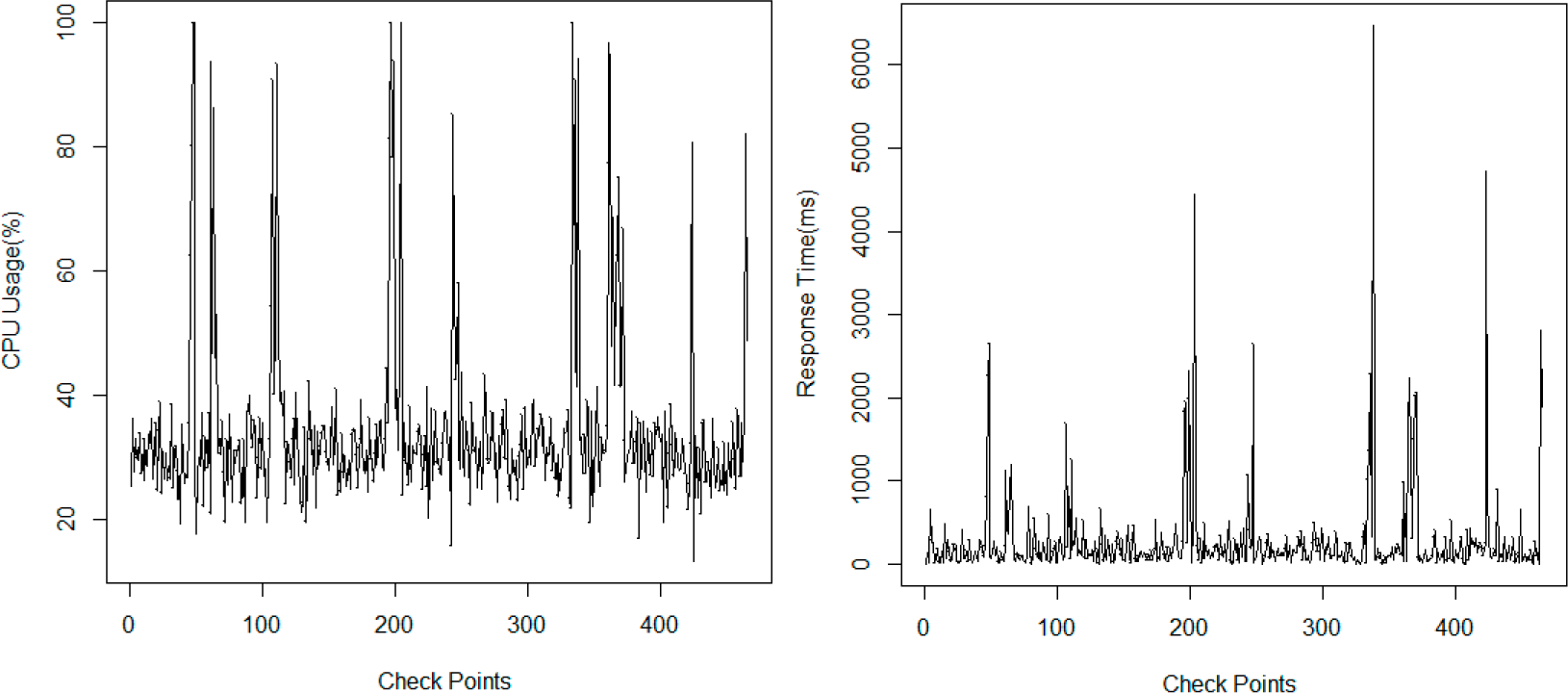
From Equation (3) we could also notice that, in order to use EWnFM, conjugate prior distributions of non-functional properties should exist as they are important for the Gibbs sampling process. Equation (3) also shows that the properties should also share the same environment states. Properties that do not share the same states would mislead the Gibbs sampling process. Algorithm 1 gives an overview of the algorithm for generating environment states. The input of the algorithm are monitor logs and the number of iterations for Gibbs sampling. Each monitor log of environment states consists of the monitor moment, the instantaneous response time and the instantaneous availability of the Web service of that moment. The output of the algorithm is the set of environment states: EnvironmentsStates, using the monitor logs as an index to record the environment state of the moment that each monitor log generates, and consisting of the parameters of the distributions of the response time and availability.

Algorithm 1. Gibbs Sampling for DPMM.

Algorithm 1. Gibbs Sampling for DPMM.

Each round of the Gibbs sampling needs to sample and generate each element in the set of environment states, while the generation of new states solely depends on the calculation and monitor logs of the last round. Therefore, sampling the elements in the set of environment states could be done with independent threads, thereby parallel computing could be used in each round of sampling to improve the efficiency of the program.

Results of the Gibbs sampling for the estimation of the model’s parameters contain two parts. Firstly, in the estimated results of ϕ_n = <λ_n,μ_n>, ϕ_n corresponds to different environment states, λ_n and μ_n are the parameters of the probabilistic distributions under each environment state, namely that the response time follows an exponential distribution of parameter λ_n, and the availability follows a normal distribution whose mean value is μ_n (assuming the variance of the normal distribution is 1). Since DPMM is a non-parametric Bayesian method, then number of different ϕ_n could be automatically determined, and counting ϕ_n could obtain the number of environment states, namely N. However, just like the other unsupervised learning algorithms, the meaning of each ϕ_n could not be given by our method. But, as we only need to estimate the number of environment states, the absence of meaning of environment states won’t affect our method. Meanwhile, [18] devised an automated way to define the context state by using context monitoring data. Secondly, considering the correspondence between the monitor logs and the environment states ϕ_n, we could acquire the transition sequences of the environment states under fixed intervals, which could be further used to estimate the parameters of the model for the transition of environment states.

2.3. Environment State Transition Matrix Estimation Method

The aforementioned section introduced a DPMM based monitor log analysis method to determine environment states and the distributions of non-functional properties under different environment states. During the execution of a Web service, the environment state transitions from one state to another, and the transitions of these states should be analyzed. As the transitions of environment states is memoryless, namely a future environment state is only associated with a current environment state, regardless of the historical environment states, therefore, continuous time Markov chain (CTMC) could be used to describe the process of environment state transition, with each states in a CTMC corresponds to an environment state. According to CTMC, the dwell time of each state follows an exponential distribution, and the dwell time and the next state are independent random variables. Generally speaking, a CTMC could be described by its initial distribution and a state transition matrix. In this paper, we only consider a relatively simple case that the initial distribution of CTMC is a steady-state distribution, thus the description of the process only requires the state transition matrix.

In a CTMC {X_t, t in T}, let p_ij(t) = P(X_t = j|X₀ = i), i,j in {X_t}. Obviously we have p_ij(t) = P(X_{t + s} = j|X_s = _i) = P(X_t = j|X₀ = i), and P = (p_ij) is usually named as the state transition probability matrix of the CTMC. Considering the previous definition of the state transition matrix of Web service environment states, the state transition matrix of environment states and the state transition probability matrix here in CTMC have the following relation:

$$P\left(t\right)={\mathrm{e}}^{\mathrm{Qt}}.$$

However, it is very difficult to analyze the such an equation, especially when the dimension of the matrix is over 3, it is almost impossible to solve the equation using conventional methods but quadratic programming, maximum likelihood estimation and Bayesian estimation, etc.[19]. On the other hand, intervals of monitor logs would also greatly affect the estimation for the state transition matrix of CTMC, and random intervals would make the estimation more complicated than fixed intervals. In this paper, considering that the historical monitor logs are acquired under fixed intervals, we adopt the Bayesian estimation based on Gibbs sampling method proposed in [20] to estimate the specific state transition matrix. Estimating parameters of CTMC based on Gibbs sampling is a kind of Markov Chain Monte Carlo method in essence. The core idea is to construct a series of CTMC ${\{Q^{(i)},Y^{(i)}\}}_{i=1}^N$ based on the monitor logs X and the posterior distribution p(Q,Y|X), in which Q⁽ⁱ⁾ and Y⁽ⁱ⁾ are intermediate results and could be used to continue constructing CTMC together with X, and then constantly generate new iterations of new CTMCs, and finally acquire a stable and traversed result. It could be considered that the expectation of the stable result represents the actual mean value depending on X and converges to Q. In order to simplify the calculation, in this paper we refer to the method in [21] to select mean values of all results to represent the estimation of Q, namely the mean value of the posterior distribution f(Q,Y) under the monitor logs X is:

$$E[f(Q,Y)|X]={\displaystyle \int f(Q,Y)p(Q,Y|X)dQdY}=\frac{{\displaystyle \sum _{i=1}^{N}f(Q^{(i)},Y^{(i)})}}{N}$$

The posterior distribution of the Bayesian formula Q could be described by a prior distribution and a likelihood function. The prior distribution of Q refers to the Gamma distribution $q_{ij}~\mathrm{\Gamma }(\frac{1}{{\beta }_i},{\alpha }_{ij})$ in [22], in which α_ij and β_i are parameters. As for the likelihood function, let Y(nτ), n in {1, 2, …, N}, represents the current transition sequence, in which τ represents the time interval of monitoring, and the number of environment states is K, thus the likelihood function could be described as:

$$\begin{array}{l}\lambda (Q)=\exp (-q_i\tau )q_{ij}\exp (-q_j\tau )q_{jk}\exp (-q_k\tau )\dots \\ ={\displaystyle \prod _{i=1}^K{\displaystyle \prod _{j\ne i}{q}_{ij}^{N_{ij}}\exp (-q_{ij}{R}_i)}}\end{array}$$

in which, R_i represents the total time for dwelling on state i and N_ij represents the total number of transitions from state i to state j in the transition sequence Y. Thus the posterior distribution of the state transition matrix Q based on the monitor sequence X and the intermediate results Y could be described as:

$$\begin{array}{l}p(Q|Y,X)\propto p(Q)p(Y|Q)\\ ={\displaystyle \prod _{i=1}^K{\displaystyle \prod _{j\ne i}{q}_{ij}^{N_{ij}+{\alpha }_{ij}-1}\exp (-q_{ij}{R}_i+{\beta }_i)}}\end{array}$$

Algorithm 2 shows an overview of the algorithm for the whole estimation process. The input of the algorithm includes transition sequence of environment states with fixed time intervals and the number of iterations NI, the output of the algorithm is the environment state transition matrix of the CTMC corresponding to the monitor logs, i.e., the infinitesimal generator matrix.

Algorithm 2. Gibbs Sampling for CTMC.

Algorithm 2. Gibbs Sampling for CTMC.

The function GenerateSequence could automatically construct a state transition sequence of intermediate results according to the parameter matrix tQ, while the function GenerateTransitionMatrix could generate a new sample of tQ based on a Gamma distribution according to the input transition sequence Ys and matrix tQ. After iterating for NI rounds, calculating for the mean values of each round’s tQ as the output, thus accomplishing the estimation for the state transition matrix of CTMC.

3. Experiments

3.1. Setup

In this paper, we choose the response time of Web services and the CPU usage of host servers as target non-functional properties to monitor simulated Web services, and model these two non-functional properties according to the monitor logs. Considering the scale of the experiment, we simulate two Web services named OperationA@h2 and OperationA@h4 in a same network, namely the same Web service OperationA was deployed on different host servers h2 and h4. An arrangement like this could eliminate impacts of network on the non-functional properties. To simulate the behavior of a web service, OperationA simply accepts a service request, delaying for a moment following an exponential distribution, and then sends back a response.

For Web service OperationA deployed in different host servers (h2, h4), since there are also many local applications and external services deployed on h2 and h4, OperationA@h2 and OperationA@h4 need to contend for limited resources with other processes on each host server. We then consider environment states corresponding to the eco state of the servers, which means that the frequency of a CPU is locked to a specific value given an eco-state. To simulate the impact of the eco state on OperationA, the parameters of the distribution of the delay time of OperationA are formed as a function of the current frequency of the host server’s CPU. We generate service requests for these two Web services respectively, generating the service requests sequence randomly according to a negative exponential distribution, and only generate new service requests after the previous response has completed. By monitoring h2 and h4 with monitors deployed in them and using SNMP based methods, we could get records of non-functional properties of Web services. The results are shown in Figures 1 and 2.

3.2. Results

On the basis of the monitor data of response time and CPU usage, we model these two non-functional properties with the simple probabilistic model, the MMPP model and the proposed EWnFM model. For the simple probabilistic model, we choose the negative exponential distribution for the response time and the normal distribution for CPU usage, evaluating parameters with the maximum likelihood estimation method and accomplishing the evaluation of parameters with Stats4 in the R language. While for the MMPP model, as MMPP is a two-dimensional exponential distribution in essence, it could only be used to analyze non-functional parameters with exponential distributions, and we only choose to model the response time, evaluating parameters using the method similar to [23], and the source code could be downloaded [24]. For the EWnFM model, as it is a multi-property description model, parameters could be evaluated using the aforementioned methods. Parameters of these two non-functional properties are shown in

Table 1. Estimation Results.

Methods	Estimations for h2	Estimations for h4
Exponential Norminal	λ = 3.56e−3 (μ,ϕ) = (34.69,14.72)	λ = 2.78e−3 (μ,ϕ) = (35.34,25.18)
MMPP	λ1 = 6.58e−3, λ2 = 0.91e−3 λ12 = 12e−4, λ21 = 1.51e−4	λ1 = 12.73e−3, λ2 = 0.87e−3 λ12 = 1.58e−4, λ21 = 10e−4
EWnFM	λ1 = 6.63e−3, λ2 = 0.83e−3 (μ1,ϕ1) = (30.46,5.02) (μ2,ϕ2) = (71.34,19.71) λ12 = 10e−4, λ21 = 1.47e−4	λ1 = 30.72e−3, λ2 = 5.58e−3, λ3 = 0.92e−3 (μ1,ϕ1) = (11.43,5.02) (μ2,ϕ2) = (31.72,13.41) (μ3,ϕ3) = (83.67,21.14) λ12 = 10.08e−4, λ13 = 0.12e−4 λ21 = 3.52e−4, λ23 = 1.78e−4 λ31 = 0.12e−4, λ32 = 5.17e−4

.

Based on Table 1, we generate 20,000 samples for each model to compare the actual monitor data with the frequency distributions of the samples. After analyzing the actual monitor data of the service OperationA@h2, we could construct a histogram frequency distribution shown in Figure 3.

While constructing models with respect to an exponential distribution of λ = 3.56 × 10⁻³ and a normal distribution of (μ,ϕ) = (34.69,14.72), 10,000 sets of data were randomly generated and frequency distributions of the samples were calculated as shown in Figure 4.

Figures 5 and 6 show the frequency distributions of 2000 randomly generated sets according to the MMPP model and the proposed EWnFM model. Obviously, for Web service OperationB@h2, the MMPP model and the EWnFM model both perform better than the simple probabilistic model.

A similar method could be used to compare the efficiency of models as for the Web service OperatioA@h4. Firstly, we analyze the actual monitor data of the Web service and show the probabilistic distribution as Figure 7. After that, models with respect to an exponential distribution of λ = 2.78 × 10⁻³ and a normal distribution of (μ,ϕ) = (34.34,25.18) are built, with 10,000 sets of data randomly generated and plotted as Figure 8. Finally, we construct an MMPP based model and an EWnFM based model with generated data shown in Figures 9 and 10.

Obviously, for Web service OperationA@h4 with three environment states, neither the simple probabilistic model nor the MMPP model could acquire results that are close to real ones. On the other hand, as the EWnFM model could automatically identify environment states of Web services, it performs much better than the other two models.

4. Conclusions and Future Works

Since (A)SBS rely on adaptation strategies to perform adaption, evaluation of these strategies is a key work to ensure the performance of (A)SBS, and a proper model of non-functional properties is fundamental for the estimation of non-functional properties and the evaluation of adaptive adaptation in (A)SBS. As Web services are in open environments, non-functional properties may be affected by many factors, which brings difficulties to the modeling of these properties. We focus on the modeling of non-functional properties of Web services in the following aspects:

• From the perspective of factors that may have impacts of non-functional properties of Web services, we proposed an environment states oriented probabilistic description model EWnFM. By introducing environment states to model non-functional properties, and based on the relations between environment states and the transfer patterns of non-functional properties, we presented a unified model for modeling non-functional properties of Web services.
• For the problem of identifying environment states, we proposed a non-parametric Bayesian based estimation method which could automatically identify environment states while simultaneously acquire the parameters of probabilistic distributions of non-functional properties under different environment states. We then introduced a Gibbs sampling based method to generate the environment state transition rate matrix. By these means, models of non-functional properties of Web services could be constructed effectively.

A key assumption in this paper is that we assume that non-functional properties are independent conditioned on environment states. This assumption is important to form conjugate prior distributions like Equation (3) since determining conjugate prior distributions for arbitrary distributions, especially joint distribution, remains a challenge. However, as non-functional properties are not always be independent, how to propose environment states oriented non-functional properties with a dependence assumption should be studied in the future. Another limitation of EWnFM is that if the distribution of the same property changes between states, it will not be applicable. DPMM, as a mixture model, could only handle a mixture of distributions sharing a same form but with different parameters. Such a limitation should also be studied if one needs to consider non-functional properties that may have different forms of distribution under different environmental states.

In this paper we considered CPU load as a non-functional property. Although we could expect that CPU load is only affected by web services under certain cases, clearly it also depends on several factors which are highly deployment-specific. As EWnFM could also be scaled to other non-functional properties, future works should also cover other kinds of properties.