Permutation Entropy for Random Binary Sequences

Abstract

In this paper, we generalize the permutation entropy (PE) measure to binary sequences, which is based on Shannon’s entropy, and theoretically analyze this measure for random binary sequences. We deduce the theoretical value of PE for random binary sequences, which can be used to measure the randomness of binary sequences. We also reveal the relationship between this PE measure with other randomness measures, such as Shannon’s entropy and Lempel–Ziv complexity. The results show that PE is consistent with these two measures. Furthermore, we use PE as one of the randomness measures to evaluate the randomness of chaotic binary sequences.

1. Introduction

Pseudorandom binary sequences play a significant role in many fields, such as error control coding, spread spectrum communications, stochastic computation, Monte Carlo simulations in numerical analysis, statistical sampling, and cryptography [1,2,3]. The sequences, which are applied to all these fields, are based on their good randomness. To test the randomness of binary sequences, some criterion have been proposed, such as SP800 [4], TestU01 [5], FIPS140-1 [6], and Crypt-XS [7]. The indexes in these test suites are combined from statistics and complexity, and, to a larger extent, from information science.

Information science considers that an information process or data sequence uses the probability measure for random states and Shannon’s entropy as the uncertainty function of these states. Very early, Fisher and Boekee proposed their information measures for maximum-likelihood estimates in statistics [8,9]. In 1948, Shannon introduced the concept of “entropy” into information science and proposes an uncertainty measure of random states [10]. Presently, Shannon’s entropy is still one of the most widely used measures to evaluate the randomness of sequences. Moreover, Renyi [11], Stratonovich [12], and Kullback and Leibler [13], all generalize Shannon’s entropy from a different perspective. Another interesting issue is the relationship between Shannon’s entropy and other complexity measures. This research is rather limited. Lempel and Ziv proposed the so-called Lempel–Ziv complexity in [14], and analyze the relationship to Shannon’s entropy. Liu revealed the relationship between Shannon’s entropy with eigenvalue and nonlinear complexity in [15,16], respectively.

In 2002, Bandt proposed a natural complexity measure for time series called permutation entropy (PE) [17]. PE is easily implemented and is computationally much faster than other comparable methods, such as Lyapunov exponents, while also being robust to noise [18], which makes it more and more popular [19,20,21,22,23,24,25,26]. In theory, the authors of [19] proposed a generalized PE based on a recently postulated entropic form and compared it to the original PE. Fan et al. [20] proposed a multiscale PE as a new complexity measure of nonlinear time series and the authors of [21] generalized it by introducing weights. Unakafova et al. [22] discussed the relationship between PE and Kolmogorov–Sinai entropy in the one-dimensional case, et al. In application, the authors of [23] used PE to quantify the nonstationarity effect in the vertical velocity records. Li et al. [24] investigated PE as a tool to predict the absence seizures of genetic absence epilepsy rats from Strasbourg. Zunino et al. [25] identified the delay time of delay dynamical system by using a PE analysis method. Mateos et al. [26] developed a PE method to characterize electrocardiograms and electroencephalographic records in the treatment of a chronic epileptic patient. PE is an interesting complexity measure based on Shannon’s entropy and can detect some phenomenons. However, it does not mean that PE is beyond Shannon’s entropy, or can completely replace it; it is just a supplement of Shannon’s entropy.

PE is a randomness measure for time series based on a comparison of neighboring values. This definition makes it difficult to apply to binary sequences. A binary sequence has only two kinds of symbols, “0” and “1”. Therefore, the comparison of neighboring values may appear as a large number or an equal sign. Almost all the applications of PE are for real number time series.

In this paper, we will generalize the PE measure to binary sequences. First, we propose a modified PE measure for binary sequences. Then, we analyze the theoretical value of PE for random binary sequences. This value can be used as one of the criterion to measure the randomness of binary sequences. Then, we will reveal the relationship between this PE measure with other randomness measure, as Shannon’s entropy and Lempel–Ziv complexity. The results show that PE is consistence with these two measures. At last, we use PE as one of the randomness measures to evaluate the randomness of chaotic binary sequences.

The rest of this paper is organized as follows. The modified PE for binary sequences and the theoretical analysis for random binary sequences are introduced in Section 2. The relationship between PE, Shannon’s entropy, and Lempel–Ziv complexity for random binary sequences are revealed in Section 3. In Section 4, we use this PE to measure the randomness of chaotic binary sequences. Finally, Section 5 concludes the paper.

2. PE and Its Theoretical Limitation for Random Binary Sequences

First, we briefly review the description in [17] for time series.

Example 1: Consider a time series with eight values x = (3 5 1 9 16 8 4 10). If order n = 2, we compare the seven pairs of neighbors. For 3 < 5, 5 > 1, 1 < 9, 9 < 16, 16 > 8, 8 > 4, and 4 < 10, then there are four of seven satisfy x_t < x_t+1, which is represented by 01, and three of seven satisfy x_t > x_t+1, which represented by 10. Then, the PE of order n = 2 can be calculated as −(4/7)log(4/7) − (3/7)log(3/7) ≈ 0.9852. If order n = 3, we compare three consecutive values. (1 9 16) is represented by 012; (3 5 1) and (9 16 8) are represented by 120; (5 1 9) and (8 4 10) are represented by 102; (16 8 4) is represented by 210. Then, the PE of order n = 3 can be calculated as −2(1/6)log(1/6) − 2(2/6)log(2/6) ≈ 1.9183. The definition of PE is described as follows.

Definition 1 

[17]: Consider a time series {x_t}_{t=1, …,T}. We study all n! permutations M of order n, which are considered here as possible order types of n different numbers. For each M, we determine the relative frequency (# means number)

$$p(M)=\frac{\#\left\{t\right|t\le T-n,(x_{t+1},\dots ,x_{t+n})\text{ has type }M\}}{T-n+1}$$

This estimates the frequency of M as good as possible for a finite series of values. The permutation entropy of order n ≥ 2 is defined as:

$$H(n)=-{\displaystyle \sum p(M)\log p(M)}$$

where the sum runs over all n! permutations M of order n.

According to Definition 1, we know that PE is a measure based on Shannon’s entropy. This measure is a supplement of Shannon’s entropy, which can detect some additional information.

Example 2: Consider a time series with sixteen values x = (4 3 2 1 3 2 1 4 2 1 4 3 2 4 3 1). By using Shannon’s entropy, the time series x is uniformly distributed, and Shannon’s entropy can be calculated as −4(1/4)log(1/4) = 2, which equals to the ideal value. This result means that the series x is an ideal random sequence in this sense. Now we calculate the PE with order n = 3. (4 3 2), (3 2 1), (3 2 1), (4 2 1), (4 3 2) and (4 3 1) are represented by 210; (2 1 3), (2 1 4), (2 1 4) and (3 2 4) are represented by 102; (1 3 2), (1 4 2) and (1 4 3) are represented by 120; (2 4 3) is represented by 021; Then, the PE of order n = 3 can be calculated as −(6/14)log(6/14) − (4/14)log(4/14) − (3/14)log(3/14) − (1/14)log(1/14) ≈ 1.7885, which is much lower than the PE of completely random sequence, as shown below. This result indicates that the series x is not an ideal random sequence with the permutation 012 and 201 never appear, which is inconsistent with the result of Shannon’s entropy.

It is clear that for a completely random sequence, where all n! possible permutations appear with the same probability, H(n) reach its maximum value logn!.

However, if the time series {x_t}_{t=1, …,T} be a binary sequences, with only two kinds of symbols “0” and “1” in its sequence, the upper theory does not hold anymore.

Let us consider the permutations M. Are there n! possible permutations in total? The answer is No! For example, consider the binary sequences consist with two 0s and two 1s. The total number of permutations should be 6, not 4!. This is because of the repeatability of symbols in the sequence. Furthermore, for a completely random binary sequence, the possible permutations will not appear with the same probability. The total number of possible permutations and their probabilities will be determined after the following definition of PE for binary sequences.

Definition 2: 

Consider a binary sequence {s_t}_{t=1, …,T}. We study all permutations M of order n, which are considered here as possible order types of n different numbers. Assume $s_{i_1},s_{i_2},\dots ,s_{i_k}$ be the 0s, and $s_{j_1},s_{j_2},\dots ,s_{j_p}$ be the 1s in sequence {s_t}, where i₁, i₂, …, i_k, j₁, j₂, …, j_p are different from each other, and k + p = T. We set $s_{i_l}=l$, 1 ≤ l ≤ k, and $s_{j_m}=m+k$, 1 ≤ m ≤ p, then, the binary sequence is transformed into a series of integer values. Calculating the relative frequency of each M as

$$p(M)=\frac{\#\left\{t\right|t\le T-n,(x_{t+1},\dots ,x_{t+n})\text{ has type }M\}}{T-n+1}$$

The permutation entropy of order n ≥ 2 is defined as:

$$H(n)=-{\displaystyle \sum p(M)\log p(M)}$$

where the sum runs over all permutations M of order n.

The main effect in Definition 2 is to transform the binary sequence into a series of integer values. For example, the sequence 000000 is transformed into 1 2 3 4 5 6, 100000 is transformed into 6 1 2 3 4 5, and 111000 is transformed into 4 5 6 1 2 3. The following example is used to describe how PE is calculated by definition 2.

Example 3: Let us take a binary sequence with nine symbols, 001010110. The PE can not be calculated by definition 1 for the consecutive repeatability of symbols in the sequence (e.g., 00 and 11). Using Definition 2, this binary sequence can be transformed into 1 2 6 3 7 4 8 9 5; therefore, no consecutive repeated symbols appear. Choose the order n = 3, we compare three consecutive values. (1 2 6) and (4 8 9) correspond to the permutation 123; (2 6 3) and (3 7 4) correspond to the permutation 132; (6 3 7) and (7 4 8) correspond to the permutation 213, and (8 9 5) correspond to the permutation 231. The PE of order n = 3 is H(3) = −3(2/7)log(2/7) − (1/7)log(1/7) ≈ 1.9502.

If the sequence {s_t} be a completely random binary sequence, PE will reach its maximum value. Consider an infinite length completely random binary sequence (i.i.d) with the probabilities of 0s and 1s be p₀ and p₁, respectively, and p₀ = p₁ = 0.5. In this case, the total number of possible permutations M should be 2ⁿ − n, and their probabilities can be calculated as follows:

$$p(1)=\frac{n+1}{2^n}$$

$$p(2)=p(3)=\dots =p(2^n-n)=\frac{1}{2^n}$$

here, p(1) is the probability of permutation “12…n”, p(2), p(3), …, p(2ⁿ − n) are the probability of other possible permutations. Put these probabilities into H(n), H(n) can be written as:

$$H(n)=-\left(\frac{n+1}{2^n}\log \frac{n+1}{2^n}+(2^n-n-1)\cdot \frac{1}{2^n}\log \frac{1}{2^n}\right)=n-\frac{n+1}{2^n}\log (n+1)$$

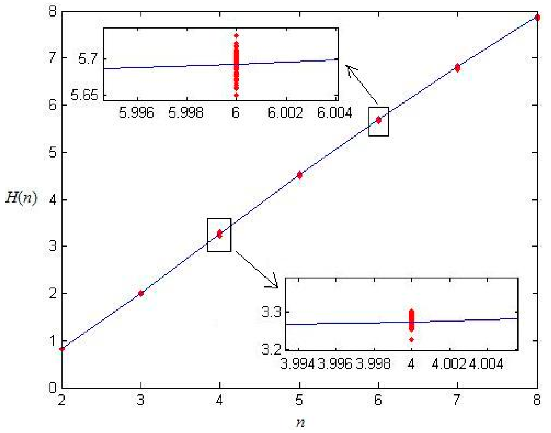
The value $n-\frac{n+1}{2^n}\log (n+1)$ is the maximum value of PE under order n for binary sequence and stands for the completely random binary sequences. In other words, a binary sequence is random if its PE is close to $n-\frac{n+1}{2^n}\log (n+1)$. We use the “rand” function in Matlab to generate 100 random binary sequences with p₀ = p₁ = 0.5; the PE values with different order n are shown in Figure 1. From Figure 1, we find that all the PE values of these binary sequences (red dots in the figure) are close to the theoretical curve (blue line in the figure), which proves our theoretical result.

Furthermore, we can generalize our result to a general random binary sequence with p₀ ≠ p₁. In this case, the total number of possible permutations M is also 2ⁿ − n, while their probabilities are different. The theoretical PE value can be written as:

$$H(n)=-\left\{\left({\displaystyle \sum _{i=0}^n{p}_0^i{p}_1^{n-i}}\right)\log \left({\displaystyle \sum _{i=0}^n{p}_0^i{p}_1^{n-i}}\right)+{\displaystyle \sum _{i=0}^n(C_n^i-1)\left(p_0^i{p}_1^{n-i}\right)\log \left(p_0^i{p}_1^{n-i}\right)}\right\}$$

here, $C_n^i=\frac{n!}{i!\cdot (n-i)!}$. If we set p₀ = p₁ = 0.5, Equation (2) will degenerate into Equation (1) since the following equation always holds:

$${\displaystyle \sum _{i=0}^n{C}_n^i}=2^n$$

Figure 1. Permutation entropy (PE) of completely random binary sequences with different n.

Figure 1. Permutation entropy (PE) of completely random binary sequences with different n.

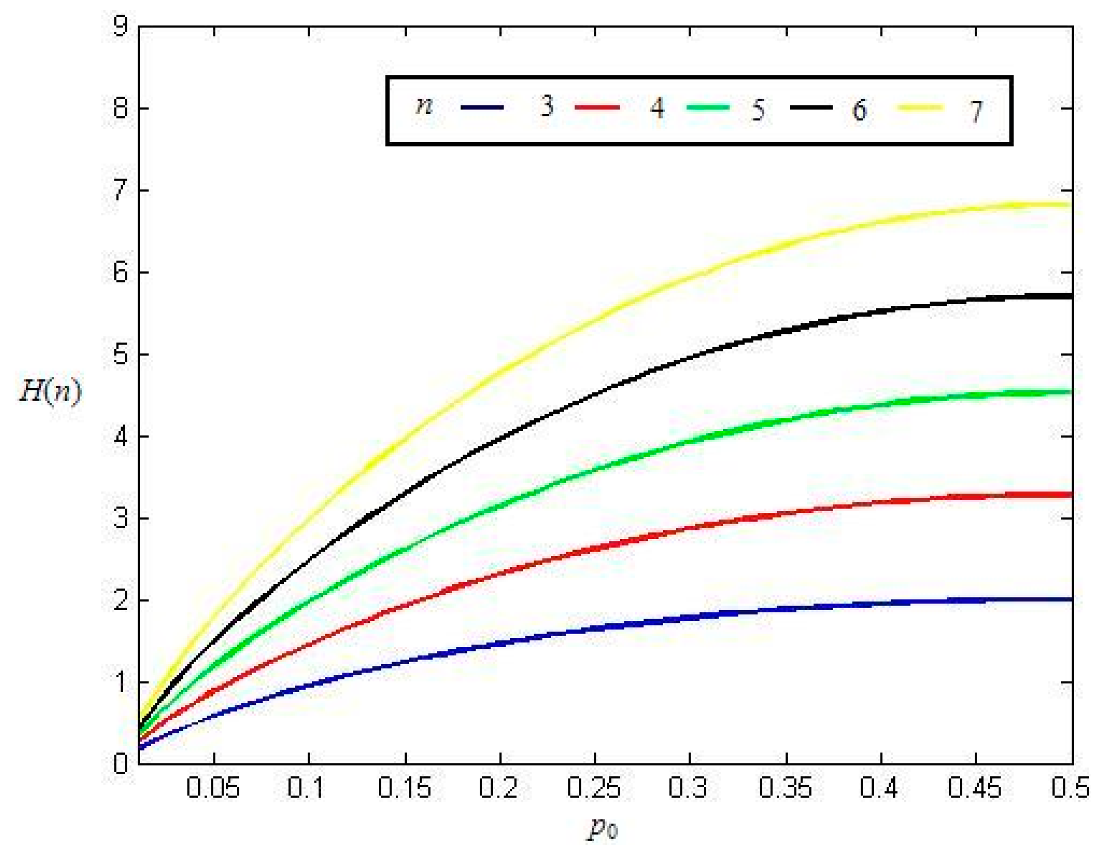
Figure 2 shows the relationship between H(n) and p₀ for different order n. From Figure 2, we can see that H(n) is increased with p₀ increases from 0 to 0.5, which is consistent to our intuition. Furthermore, the larger the order n is, the larger the H(n) is. For different n, the curves are similar and only have the difference on the magnitude. Therefore, we say PE is robust to its order n.

Figure 2. The relationship between H(n) and p₀ for different order n of random binary sequences.

Figure 2. The relationship between H(n) and p₀ for different order n of random binary sequences.

3. Relation to Shannon’s Entropy and Lempel–Ziv Complexity for Random Binary Sequences

Some measures have been proposed and used for measuring the randomness of binary sequences for decades, such as Shannon’s entropy and Lempel–Ziv complexity. In this section, we will reveal the relationship between PE and these two measures. For the robustness of order n, we set n = 6 in the following numerical experiments.

3.1. Connections to Shannon’s Entropy

Shannon’s entropy is used to measure the uncertainty of random states and is defined as:

$$h=-{\displaystyle \sum _i{p}_i\log p_i}$$

where p_i is the probability of state i. For binary sequences, we have i = 0, 1. We totally generate 100 groups of random binary sequences with different p₀. After calculating their PE values and Shannon’s entropies, the relationship is shown in Figure 3. Figure 3 indicates that there is an approximately linear relation between PE and Shannon’s entropy.

Figure 3. The relationship between PE and Shannon’s entropy.

Figure 3. The relationship between PE and Shannon’s entropy.

The linear curve can be written as follows:

$$\text{PE}=5.858h-0.2205$$

The numerical coefficients in this linear function are approximately estimated by using the least square method. Two criterions are used to show that our fitting result is quite good. The coefficient of determination is 0.9982, and the root mean squared error is 0.06718.

3.2. Connections to Lempel–Ziv Complexity

Lempel–Ziv complexity was proposed by Lempel and Ziv [14], which is related to the number of distinct phrases and the rate of their occurrence along the sequence. Lempel–Ziv complexity is related to the sequence length. Therefore, we should first do normalization.

For a n-length random binary sequence, the expectation of the Lempel–Ziv complexity is n/log₂n. We denote b(n) = n/log₂n, normalize Lempel–Ziv complexity with b(n) as:

D(n) = LZ(n)/b(n)

Then, the complexity of this sequence can be measured with the normalized D(n). If the D(n) of a given sequence approaches to 1, the sequence is regarded as a true random one.

We also generate 100 groups of random binary sequences with different p₀. After calculating their PE values and Lempel–Ziv complexity, the relationship is shown in Figure 4. From Figure 4 we can see that PE is also approximately linear with the normalized Lempel–Ziv complexity.

The linear curve can be written as follows:

$$\text{PE}=5.548D(n)-0.09805$$

Additionally, the numerical coefficients are approximately estimated by using the least square method. The coefficient of determination is 0.9987, and the root mean squared error is 0.05709, which means that our fitting result is quite good.

Figure 4. The relationship between PE and Lempel–Ziv complexity.

Figure 4. The relationship between PE and Lempel–Ziv complexity.

In summary for binary sequences, PE is approximately linear with Shannon’s entropy and Lempel–Ziv complexity. As shown in [17], in contrast with all known complexity measures, the calculation of PE is extremely fast and robust, and seems preferable than other complexity measures especially with huge data sets.

4. PE as One of the Randomness Measures

As analyzed above, PE can be used as one of the randomness measure for binary sequences. In this section, we will use PE to evaluate the randomness of chaotic binary sequences. Three kinds of chaotic systems are used here including the Logistic map, Tent map and Baker map.

4.1. Logistic Map

The Logistic map is a typical chaotic systems. The function of the Logistic map is as follows:

$$x_{n+1}=r{x}_n(1-x_n)$$

where, r is the degree of the Logistic map. For 3.5699 < r ≤ 4, it can generate a chaotic pseudorandom real-valued sequence for almost any initial value. For r = 4, the generating partition is the critical value 0.5.

4.2. Tent Map

The function of the Tent map is given as follows:

$$x_{n+1}=\{\begin{array}{ll}{x}_n/h,& 0<x\le h\\ (1-x_n)/(1-h),& h<x\le 1\end{array}$$

where, h is the coefficient of the Tent map. For 0 < h < 1, this map becomes chaotic.

4.3. Baker Map

The function of the Baker map is given as follows:

$$(x_{n+1},y_{n+1})=\{\begin{array}{ll}(x_n/p,p{y}_n)& 0<x\le p\\ ((x_n-p)/(1-p),(1-p)y_n+1-p)& p<x\le 1\end{array}$$

Here, p is the degree of the Baker map. For 0 < p < 1, this map will become chaotic. The Baker map is widely used in image encryption algorithm.

The following frequently-used binary quantification algorithm is used to generate the chaotic binary sequences:

$$b_n=\{\begin{array}{ll}0,& x_n\le U_0\\ 1,& x_n>U_0\end{array}$$

where U₀ is the critical value, x_n is the chaotic real value. For the two-dimensional Baker map, the x-dimensional chaotic sequence is selected as the experimental sample in this paper.

Figure 5a shows the PE values with order n = 6 of Logistic chaotic binary sequences with different parameters. The standard line PE = 5.6929 is the maximum value of PE under order 6 for binary sequence, which can be calculated by Equation (1). Figure 5a,b indicates that the PE curve is approximately similar to the positive Lyapunov exponent of Logistic maps. It is also can be seen in [17].

Figure 6 shows the PE values with order n = 6 of Tent chaotic binary sequences with different parameters. From Figure 6, we have that if the parameter h locates near the value 0.1 or 0.4, PE will quickly tend to zero. Furthermore, PE will approach to the theoretical value of completely random sequences with h increasing to the value 0.5. Therefore, the Tent chaotic binary sequences have good randomness properties in this sense, once h is close to 0.5. Figure 7 shows the PE values with order n = 6 of Baker chaotic binary sequences with different parameters. Figure 7 indicates that if the parameter p locates near the value 0.1, PE will quickly tend to zero. With other parameters, PE will roughly increase with p and will approach to the theoretical value of completely random sequences, which means that if the parameter p is close to 0.5, the generated binary sequences are with good randomness in this sense.

Figure 5. PE (a) and Lyapunov exponent (b) of Logistic chaotic binary sequences with different parameters.

Figure 5. PE (a) and Lyapunov exponent (b) of Logistic chaotic binary sequences with different parameters.

Figure 6. PE of Tent chaotic binary sequences with different parameters.

Figure 6. PE of Tent chaotic binary sequences with different parameters.

Figure 7. PE of Baker chaotic binary sequences with different parameters.

Figure 7. PE of Baker chaotic binary sequences with different parameters.

5. Conclusions

Permutation entropy is a natural complexity measure for time series which has been widely used recently. In this paper, we generalize the PE measure to binary sequences. The theoretical value of PE for random binary sequences is given by both theoretical and experimental analysis. Additionally, we establish the relationship between PE with Shannon’s entropy and Lempel–Ziv complexity. The results show that PE is approximately linear with these two measures. Furthermore, we use PE as one of the randomness measures to evaluate the randomness of three kinds of chaotic binary sequences, which is consistent with the existing results.

References

1. Kalouptsidis, N. Signal Processing Systems: Theory and Design; Telecommunications and Signal Processing Series; Wiley: New York, NY, USA, 1996. [Google Scholar]
2. Golomb, S.W. Shift Register Sequences; Holden-Day: San Francisco, CA, USA, 1967. [Google Scholar]
3. Wang, X.M.; Zhang, W.F.; Guo, W.; Zhang, J.S. Secure chaotic system with application to chaotic ciphers. Inf. Sci. 2013, 221, 555–570. [Google Scholar] [CrossRef]
4. Rukin, A.; Soto, J.; Nechvatal, J.; Smid, M.; Barker, E. A Statistical Test Suite for Random and Pseudorandom Number Generators for Cryptographic Applications; NIST (National Institute of Standards and Technology): Gaithersburg, MD, USA, 2001. [Google Scholar]
5. Ecuyer, P.L.; Simard, R. TestU01: A C library for empirical testing of random number generators. ACM Trans. Math. Softw. 2007, 33, 1–22. [Google Scholar] [CrossRef]
6. Security Requirements for Cryptographic Modules. Federal Information Processing Standards Publication (FIPS140–1); NIST (National Institute of Standards and Technology): Gaithersburg, MD, USA, 1994.
7. Gustafson, H.; Dawson, E.; Nielsen, L.; Caelli, W. A computer package for measuring the strength of encryption algorithms. J. Comput. Secur. 1994, 13, 687–697. [Google Scholar] [CrossRef]
8. Fisher, R.A. On the mathematical foundations of theoretical statistics. Philos. Trans. R. Soc. A 1922, 222, 309–368. [Google Scholar] [CrossRef]
9. Boekee, D.E. An extension of the Fisher Information Measure. Annu. Rev. Top. Inf. Theory 1977, 16, 493–519. [Google Scholar]
10. Shannon, C.E.; Weaver, E. The Mathematical Theory of Communication; Illinois Press: Urbana, IL, USA, 1949. [Google Scholar]
11. Renyi, A. On Measures of Entropy and Information. In Proceedings of the 4th Berkeley Symposium on Mathematics Statistics and Probability; University of California Press: Berkeley, CA, USA, 1960; pp. 547–561. [Google Scholar]
12. Stratonovich, R.L. Theory of Information; Sov. Radio: Moscow, Russia, 1975. [Google Scholar]
13. Kullback, S. Information Theory and Statistics; Wiley and Sons: New York, NY, USA, 1959. [Google Scholar]
14. Lempel, A.; Ziv, J. On the complexity of finite sequences. IEEE Trans. Inf. Theory 1976, 22, 75–81. [Google Scholar] [CrossRef]
15. Liu, L.F.; Miao, S.X.; Hu, H.P.; Deng, Y.S. On the eigenvalue and Shannon’s entropy of finite length random sequences. Complexity 2014. [Google Scholar] [CrossRef]
16. Liu, L.F.; Miao, S.X.; Liu, B.C. On nonlinear complexity and Shannon’s entropy of finite length random sequences. Entropy 2015, 17, 1936–1945. [Google Scholar] [CrossRef]
17. Bandt, C.; Pompe, B. Permutation entropy: A natural complexity measure for time series. Phys. Rev. Lett. 2002, 88, 174102. [Google Scholar] [CrossRef] [PubMed]
18. Toomey, J.; Kane, D. Mapping the dynamic complexity of a semiconductor laser with optical feedback using permutation entropy. Opt. Express 2014, 22, 1713–1725. [Google Scholar] [CrossRef] [PubMed]
19. Xu, M.J.; Shang, P.J. Generalized permutation entropy analysis based on the two-index entropic form Sq,δ. Chaos 2015, 25, 053114. [Google Scholar] [CrossRef] [PubMed]
20. Fan, C.L.; Jin, N.D.; Chen, X.T.; Gao, Z.K. Multi-scale permutation entropy: A complexity measure for discriminating two-phase flow dynamics. Chin. Phys. Lett. 2013, 30, 090501. [Google Scholar] [CrossRef]
21. Yin, Y.; Shang, P.J. Weighted multiscale permutation entropy of financial time series. Nonlinear Dyn. 2014, 78, 2921–2939. [Google Scholar] [CrossRef]
22. Unakafova, V.A.; Unakafov, A.M.; Keller, K. An approach to comparing Kolmogorov-Sinai and permutation entropy. Eur. Phys. J. Spec. Top. 2013, 222, 353–361. [Google Scholar] [CrossRef]
23. Li, Q.L.; Fu, Z.T. Permutation entropy and statistical complexity quantifier of nonstationarity effect in the vertical velocity records. Phys. Rev. E 2014, 89, 012905. [Google Scholar] [CrossRef] [PubMed]
24. Li, X.L.; Ouyang, G.X.; Richards, D.A. Predictability analysis of absence seizures with permutation entropy. Epilepsy Res. 2007, 77, 70–74. [Google Scholar] [CrossRef] [PubMed]
25. Zunino, L.; Soriano, M.C.; Fischer, I.; Rosso, O.A.; Mirasso, C.R. Permutation-information-theory approach to unveil delay dynamics form time-series analysis. Phys. Rev. E 2010, 82, 046212. [Google Scholar] [CrossRef] [PubMed]
26. Mateos, D.; Diaz, J.M.; Lamberti, P.W. Permutation Entropy Applied to the Characterization of the Clinical Evolution of Epileptic Patients under Pharmacological Treatment. Entropy 2014, 16, 5668–5676. [Google Scholar] [CrossRef]