Thermal BEC Black Holes

Abstract

We review some features of Bose–Einstein condensate (BEC) models of black holes obtained by means of the horizon wave function formalism. We consider the Klein–Gordon equation for a toy graviton field coupled to a static matter current in a spherically-symmetric setup. The classical field reproduces the Newtonian potential generated by the matter source, while the corresponding quantum state is given by a coherent superposition of scalar modes with a continuous occupation number. An attractive self-interaction is needed for bound states to form, the case in which one finds that (approximately) one mode is allowed, and the system of N bosons can be self-confined in a volume of the size of the Schwarzschild radius. The horizon wave function formalism is then used to show that the radius of such a system corresponds to a proper horizon. The uncertainty in the size of the horizon is related to the typical energy of Hawking modes: it decreases with the increasing of the black hole mass (larger number of gravitons), resulting in agreement with the semiclassical calculations and which does not hold for a single very massive particle. The spectrum of these systems has two components: a discrete ground state of energy m (the bosons forming the black hole) and a continuous spectrum with energy $\omega >m$ (representing the Hawking radiation and modeled with a Planckian distribution at the expected Hawking temperature). Assuming the main effect of the internal scatterings is the Hawking radiation, the N-particle state can be collectively described by a single-particle wave-function given by a superposition of a total ground state with energy $M=Nm$ and a Planckian distribution for $E>M$ at the same Hawking temperature. This can be used to compute the partition function and to find the usual area law for the entropy, with a logarithmic correction related to the Hawking component. The backreaction of modes with $\omega >m$ is also shown to reduce the Hawking flux. The above corrections suggest that for black holes in this quantum state, the evaporation properly stops for a vanishing mass.

1. Introduction

Unreachable, untestable and directly unobservable, black holes are among the most intriguing and discussed theoretical predictions of modern physics. Strong evidence exists that these obscure hollows in the space-time structure are indeed generated when the life of very massive stars comes to an end. Oppenheimer and co-workers [1,2] were the pioneers in the field of stellar collapse, and since then, the scientific production of this subject has known an endless growth, exposing many obscure points in general relativity and leaving many questions unanswered (see [3,4] and the references therein, for example). Problems get even more arduous if quantum mechanics is taken into account when considering the formation of black holes. Both at macroscopic and microscopic scales, one usually turns to Thorne’s so-called hoop conjecture [5], which states that a black hole is formed whenever a given mass (or equivalent energy) M is entirely confined inside its corresponding gravitational radius $R_{\mathrm{H}}$. We recall that, in the simplest cases, this is just the Schwarzschild radius $R_{\mathrm{H}}=2G_{\mathrm{N}}M$, where $G_{\mathrm{N}}={\ell }_{\mathrm{p}}/m_{\mathrm{p}}$, and ${\ell }_{\mathrm{p}}$ and $m_{\mathrm{p}}$ are the Planck length and mass, respectively, so that $\hslash ={\ell }_{\mathrm{p}}{m}_{\mathrm{p}}$ (we shall of course use units with $c=1$). Initially formulated for macroscopic black holes [6,7,8], the hoop conjecture lacks a solid experimental proof, but from a theoretical perspective, it turns out to be solid and reliable on different testing grounds. In the classical domain of very large systems, the very concept of a background metric and related horizon structure are well understood (for a review of some problems, see the bibliography in [9]). Going down to the Planck scale, however, concepts, such as the particle’s “size” and “position”, become fuzzy, and this makes the hoop conjecture much more difficult to state clearly. In this range, quantum effects are relevant (for a recent discussion, see, e.g., [10]), and one should also consider the possible existence of new objects, usually referred to as “quantum black holes” (see, e.g., [11,12,13]). The idea that black holes may originate in particle collisions is supported by the hoop conjecture itself. Two particles (with, say, negligible spatial extension and total angular momentum) can collide with an impact parameter b shorter than the Schwarzschild radius corresponding to the total center-of-mass energy E of the system,

$$\begin{array}{c}\hfill b\le 2{\ell }_{\mathrm{p}}\frac{E}{m_{\mathrm{p}}}\equiv R_{\mathrm{H}}(E)\end{array}$$

(1)

One then expects that a microscopic black hole is formed, with non-negligible quantum properties. Because of this, black holes would require a quantum theory of gravity in order to be described and studied properly. Such a (universally-accepted) theory does not yet exist, and one has to work under (sometimes strong) approximations. Quantum field theory on curved space-time backgrounds has been developed for this purpose: this theoretical approach relies on the assumption that quantum gravitational fluctuations are small and has produced remarkable results [14,15].

A new theoretical model was recently proposed by Dvali and Gomez [16,17,18,19,20,21,22], which allows one to describe the quantum properties of black holes from an entirely new perspective: large black holes are viewed as graviton condensates at a critical point and can be reliably described on flat space, the curved metric emerging as a collective effect. The aim of this review is to present some of the features of this model obtained from the “horizon wave-function formalism” (HWF). In this general approach, a wave-function for the gravitational radius can be associated with any localized quantum mechanical particle [23,24,25,26,27,28], which makes it easy to formulate in a quantitative way a condition for distinguishing black holes from regular particles. Among the added values, the formalism naturally leads to an effective generalized uncertainty principle (GUP) [29,30,31,32,33] for the particle’s position (similar features are naturally encoded in non-commutative models of black holes; for a review, see [34]), and a decay rate for microscopic black holes.

In the next section, we briefly review the corpuscular model of [16,17,18,19,20,21,22] and one of its possible field theoretic implementations in Section 3 (the particular case we consider there will allow us to make some conjectures regarding the black hole formation from the gravitational collapse of a star). In Section 4, we review the HWF and how it reproduces a GUP. This formalism is then applied to specific models of corpuscular black holes and their Hawking radiation in Section 5, which is the main part of this review, and collects results from [35] and [36]. Finally, some comments and speculations are summarized in Section 6.

2. Corpuscular Model

The simple and intuitive corpuscular model recently introduced by Dvali and Gomez in [16,17,18,19,20,21,22] and widely developed in [36,37,38,39,40,41,42,43,44], puts gravitation under a new light. The model is based on the assumption that the classical geometry should be viewed as an effective description of a quantum state with a large graviton occupation number, where gravitons play the role of space-time quanta, very much like photons are light quanta in a laser beam. Unlike photons, which do not interact with each other via quantum electrodynamics, the graviton-graviton interaction is mediated by gravitation itself, whose attractive nature can thus lead to forming a ball of superposed gravitational quanta. When such a superposition is a ground state, the gravitational field is effectively a Bose–Einstein condensate (BEC): Dvali and Gomez conjectured that this is precisely what happens inside black holes. Even when considering a strong gravitational regime, as expected to happen at the verge of black hole formation, the whole construction can be nicely explained under Newtonian approximation. The Newtonian potential at a distance r generated by a system of N gravitons, each with effective mass m (so that the total mass $M=Nm$), is:

$$\begin{array}{c}\hfill V_{\mathrm{N}}(r)\simeq -\frac{G_{\mathrm{N}}M}{r}=-\frac{{\ell }_{\mathrm{p}}Nm}{r{m}_{\mathrm{p}}}\end{array}$$

(2)

This potential can be strong enough to confine the gravitons themselves inside a finite volume where they are all superposed on each other. The gravitons effective mass m can be related to their characteristic quantum mechanical size via the Compton/de Broglie wavelength ${\lambda }_m\simeq \frac{\hslash }{m}={\ell }_{\mathrm{p}}\frac{m_{\mathrm{p}}}{m}$. If one assumes that the interaction is negligible outside the ball of gravitons and constant inside, with average interaction distance $r={\lambda }_m$, the potential simplifies to:

$$\begin{array}{c}\hfill V_{\mathrm{N}}(r)\simeq -\frac{G_{\mathrm{N}}M}{{\lambda }_m}\Theta ({\lambda }_m-r):=V_{\mathrm{N}}({\lambda }_m)\end{array}$$

(3)

which results in an average potential energy per graviton:

$$\begin{array}{c}\hfill U_m\simeq m{V}_{\mathrm{N}}({\lambda }_m):=-N\alpha m\end{array}$$

(4)

where:

$$\begin{array}{c}\hfill \alpha =\frac{{\ell }_{\mathrm{p}}^2}{{\lambda }_m^2}=\frac{m^2}{m_{\mathrm{p}}^2}\end{array}$$

(5)

is the gravitational coupling.

One can think of virtually superposing gravitons one by one, thus strengthening their reciprocal attraction, until they find themselves confined inside a deep enough “potential well” from which they cannot escape. The condition for the gravitons to be “marginally bound” is reached when each single graviton has just not enough energy $E_K=m$ to escape the potential well,

$$\begin{array}{c}\hfill E_K+U\simeq 0\end{array}$$

(6)

At this point, one has created a black hole solely out of condensed gravitational quanta. When this condition is reached, the gravitons are ”maximally packed”, and their number satisfies:

$$\begin{array}{c}\hfill N\alpha \simeq 1\end{array}$$

(7)

The effective graviton mass correspondingly scales as:

$$\begin{array}{c}\hfill m\simeq \frac{m_{\mathrm{p}}}{\sqrt{N}}\end{array}$$

(8)

while the total mass of the black hole scales like (this scaling relation had been already found in [45] without fully understanding its role in the case of black hole formation):

$$\begin{array}{c}\hfill M=Nm\simeq \sqrt{N}{m}_{\mathrm{p}}\end{array}$$

(9)

Moreover, the horizon’s size, namely the Schwarzschild radius:

$$\begin{array}{c}\hfill R_{\mathrm{H}}=2{\ell }_{\mathrm{p}}\frac{M}{m_{\mathrm{p}}}\end{array}$$

(10)

is spontaneously quantized as commonly expected [46], that is:

$$\begin{array}{c}\hfill R_{\mathrm{H}}\simeq \sqrt{N}{\ell }_{\mathrm{p}}\end{array}$$

(11)

This simple, purely gravitational black hole can now be shown to emit purely gravitational Hawking radiation. In a first order approximation, reciprocal $2\to 2$ graviton scatterings inside the condensate will give rise to a depletion rate:

$$\begin{array}{c}\hfill \Gamma \sim \frac{1}{N^2}{N}^2\frac{1}{\sqrt{N}{\ell }_{\mathrm{p}}}\end{array}$$

(12)

where the factor $N^{-2}$ comes from ${\alpha }^2$, the second factor is combinatoric (there are about N gravitons scattering with other $N-1\simeq N$ gravitons) and the last factor comes from the characteristic energy of the process $\Delta E\sim m$. The amount of gravitons in the condensate will then decrease according to [16,17,18,19,20,21,22]:

$$\begin{array}{c}\hfill \dot{N}\simeq -\Gamma \simeq -\frac{1}{\sqrt{N}{\ell }_{\mathrm{p}}}+O(N^{-1})\end{array}$$

(13)

As explained in [16,17,18,19,20,21,22], this emission of gravitons reproduces the purely gravitational part of the Hawking radiation and contributes to the shrinking of the black hole according to the standard results:

$$\begin{array}{c}\hfill \dot{M}\simeq m_{\mathrm{p}}\frac{\dot{N}}{\sqrt{N}}\sim -\frac{m_{\mathrm{p}}}{N{\ell }_{\mathrm{p}}}\sim -\frac{m_{\mathrm{p}}^3}{{\ell }_{\mathrm{p}}{M}^2}\end{array}$$

(14)

From this flux, one can then read off the “effective” Hawking temperature:

$$\begin{array}{c}\hfill T_{\mathrm{H}}\simeq \frac{m_{\mathrm{p}}^2}{8\pi M}\sim m\sim \frac{m_{\mathrm{p}}}{\sqrt{N}}\end{array}$$

(15)

where the last expression is precisely the approximate value we shall use throughout.

Let us remark once more that this BEC model only contains gravity, and the Hawking radiation we consider here is therefore just the graviton contribution. In a more refined model, one would also like to include all possible matter content (presumably originating from the astrophysical object that collapsed to form the black hole) and hopefully recover all types of radiation (for some preliminary results regarding the role of baryons, see [47]).

3. Scalar Toy Gravitons Coupled to A Source

The model presented in the previous section is very simple and leads to very “reasonable” properties, but in its original form lacks some features that might make it even more appealing. For example, the connection with the usual geometrical picture of general relativity is not immediate, and the horizon “emerges” from a classical mechanical condition (the binding condition of Equation (6)), rather than from relativistic considerations (as happens in the case of the hoop conjecture).

Trying to understand the corpuscular theory of Dvali and Gomez, using different tools can be of some help. In [35], quantum field Theory was proposed in order to model a self-sustained graviton system. To simplify the description, the authors consider scalar toy-gravitons instead of regular gravitons, which allows one to employ the Klein–Gordon equation for a real and massless scalar field ϕ coupled to a real scalar current J in Minkowski space-time,

$$\begin{array}{c}\hfill \square \varphi (x)=qJ(x)\end{array}$$

(16)

where $\square ={\eta }^{\mu \nu }{\partial }_{\mu }{\partial }_{\nu }$ and q is a dimensionless coupling. One then also assumes that the current is time-independent, ${\partial }_{0}J=0$. In momentum space, with $k^{\mu }=(k^0,\mathbf{k})$, this leads to:

$$\begin{array}{c}\hfill k^0\tilde{J}(k^{\mu })=0\end{array}$$

(17)

which is solved by the distribution:

$$\begin{array}{c}\hfill \tilde{J}(k^{\mu })=2\pi \delta (k^0)\tilde{J}(\mathbf{k})\end{array}$$

(18)

where ${\tilde{J}}^{*}(\mathbf{k})=\tilde{J}(-\mathbf{k})$. For the spatial part, exact spherical symmetry is assumed, so that the analysis is restricted to functions of the kind $f(\mathbf{x})=f(r)$, with $r=|\mathbf{x}|$. Classical spherically symmetric solutions of Equation (16) can be formally written as:

$$\begin{array}{c}\hfill {\varphi }_{\mathrm{c}}(r)=q{\square }^{-1}J(r)\end{array}$$

(19)

and they can be found more easily in momentum space. The latter is defined by the integral transformation:

$$\begin{array}{c}\hfill \tilde{f}(k)=4\pi {\int }_0^{+\infty }dr{r}^2{j}_0(kr)f(r)\end{array}$$

(20)

where:

$$\begin{array}{c}\hfill j_0(kr)=\frac{sin(kr)}{kr}\end{array}$$

(21)

is a spherical Bessel function of the first kind and $k=|\mathbf{k}|$. This gives the solution:

$$\begin{array}{c}\hfill {\tilde{\varphi }}_{\mathrm{c}}(k)=-q\frac{\tilde{J}(k)}{k^2}\end{array}$$

(22)

For example, for a current with Gaussian profile,

$$\begin{array}{c}\hfill J(r)=\frac{e^{-r^2/(2{\sigma }^2)}}{{(2\pi {\sigma }^2)}^{3/2}}\end{array}$$

(23)

one finds:

$$\begin{array}{c}\hfill \tilde{J}(k)=e^{-k^2{\sigma }^2/2}\end{array}$$

(24)

and the corresponding classical scalar field is given by:

$$\begin{array}{ccc}\hfill {\varphi }_{\mathrm{c}}(r)& =& -\frac{q}{2{\pi }^2}{\int }_0^{+\infty }\mathrm{d}k{j}_0(kr)e^{-k^2{\sigma }^2/2}\hfill \\ & =& -\frac{q}{4\pi r}\mathrm{erf}\left(\frac{r}{\sqrt{2}\sigma }\right)\hfill \end{array}$$

(25)

where $\mathrm{erf}$ is the error function. At large distances from the source J, when $r\gg \sigma$, the field ϕ reproduces the classical Newtonian potential Equation (2), i.e.,

$$\begin{array}{c}\hfill V_{\mathrm{N}}=\frac{4\pi }{q}{G}_{\mathrm{N}}M{\varphi }_{\mathrm{c}}\simeq -\frac{G_{\mathrm{N}}M}{r}\end{array}$$

(26)

In the quantum theory, the classical configurations Equation (19) are replaced by coherent states. To prove this statement, one can start with the normal-ordered quantum Hamiltonian density in momentum space,

$$\begin{array}{c}\hfill \widehat{\mathcal{H}}=k{\widehat{a}}_k^{\prime †}{\widehat{a}}_k^{\prime }+{\tilde{\mathcal{H}}}_g\end{array}$$

(27)

where ${\tilde{\mathcal{H}}}_g$ is the ground state energy density,

$$\begin{array}{c}\hfill {\tilde{\mathcal{H}}}_g=-q^2\frac{|\tilde{J}{(k)|}^2}{2k^2}\end{array}$$

(28)

and the standard ladder operators are shifted according to:

$$\begin{array}{c}\hfill {\widehat{a}}_k^{\prime }={\widehat{a}}_k+q\frac{\tilde{J}(k)}{\sqrt{2k^3}}\end{array}$$

(29)

The source-dependent ground state $\left|g\right.〉$ is annihilated by the shifted annihilation operator,

$$\begin{array}{c}\hfill {\widehat{a}}_k^{\prime }\left|g\right.〉=0\end{array}$$

(30)

and is a coherent state in terms of the standard field vacuum,

$$\begin{array}{c}\hfill {\widehat{a}}_k\left|g\right.〉=-q\frac{\tilde{J}(k)}{\sqrt{2k^3}}\left|g\right.〉=g(k)\left|g\right.〉\end{array}$$

(31)

with $g=g(k)$ being an eigenvalue of the shifted annihilation operator. This results in:

$$\begin{array}{c}\hfill \left|g\right.〉=e^{-N/2}\exp \left\{\int \frac{k^2\mathrm{d}k}{2{\pi }^2}g(k){\widehat{a}}_k^{†}\right\}\left|0\right.〉\end{array}$$

(32)

with N representing the expectation value of the number of quanta in the coherent state,

$$\begin{array}{ccc}\hfill N& =& \int \frac{k^2\mathrm{d}k}{2{\pi }^2}\left.〈g\right|{\widehat{a}}_k^{†}{\widehat{a}}_k\left|g\right.〉\hfill \\ & =& \frac{q^2}{{(2\pi )}^2}\int \frac{\mathrm{d}k}{k}{|\tilde{J}(k)|}^2\hfill \end{array}$$

(33)

from which the occupation number is found to be:

$$\begin{array}{c}\hfill n_k={\left(\frac{q}{2\pi }\right)}^2\frac{|\tilde{J}{(k)|}^2}{k}\end{array}$$

(34)

It is now straightforward to verify that the expectation value of the field in the state $\left|g\right.〉$ coincides with its classical value,

$$\begin{array}{ccc}\hfill \left.〈g\right|{\widehat{\varphi }}_k\left|g\right.〉& =& \frac{1}{\sqrt{2k}}\left.〈g\right|\left({\widehat{a}}_k+{\widehat{a}}_{-k}^{†}\right)\left|g\right.〉\hfill \\ & =& \frac{1}{\sqrt{2k}}\left.〈g\right|\left({\widehat{a}}_k^{\prime }+{\widehat{a}}_{-k}^{\prime †}\right)\left|g\right.〉-q\frac{\tilde{J}(k)}{k^2}\hfill \\ & =& {\tilde{\varphi }}_{\mathrm{c}}(k)\hfill \end{array}$$

(35)

thus $|g\rangle$ is a realization of the Ehrenfest theorem.

It is important to note that Equation (33) presents a UV divergence if the source has infinitely thin support and an IR divergence if the source contains modes of vanishing momenta (which would only be physically consistent with an eternal source). Because of this, the state $\left|g\right.〉$ and the number N are not mathematically well defined in general. Anyway, the UV divergence can be cured, for example, by using a Gaussian distribution, like the one in Equation (23), while the IR divergence can be eliminated if the scalar field is massive or the system is enclosed within a finite volume (so that allowed modes are also quantized).

3.1. Black Holes as Self-Sustained Quantum States

One can now analyze a “star”, made of ordinary matter whose density is distributed according to:

$$\begin{array}{c}\hfill \rho =MJ\end{array}$$

(36)

where M is the total (proper) energy of the star. Its Newtonian potential energy is given by $U_M=M{V}_{\mathrm{N}}$, so that ${\varphi }_{\mathrm{c}}$ is accordingly determined by Equation (26) and the quantum state of $\widehat{\varphi }$ by Equation (35).

During the formation of a black hole, the gravitons are expected to dominate the dynamics over the matter source [16,17,18,19,20,21,22]. Then, one can assume the matter contribution is negligible, and the source J in the r.h.s. of Equation (16) is thus provided by the gravitons themselves. This source, consisting of gravitons, is roughly confined in a finite spherical volume $\mathcal{V}=4\pi R^3/3$ (this is a crucial feature for the “classicalization” of gravity [48,49] and requires an attractive self-interaction for the scalar field to admit bound states). The energy density Equation (36) must then be equal to the average energy density inside the volume $\mathcal{V}$, which, in turn, is given by the average potential energy of each graviton in $\mathcal{V}$, times the number of gravitons: $N{U}_m/\mathcal{V}$ (each graviton interacts with the other $N-1$, so that the energy of each graviton is proportional to $(N-1)U_m$, but one can safely approximate $N-1\simeq N$, given that N is considered large). This assumption is qualitatively the same as the marginally-bound condition Equation (6) with $N{E}_{\mathrm{K}}\sim J$. After some simple substitutions, one finds:

$$\begin{array}{c}\hfill J\simeq -\frac{3N{G}_{\mathrm{N}}m}{q{R}^3}{\varphi }_{\mathrm{c}}\end{array}$$

(37)

inside the volume $\mathcal{V}$, where m is the energy of each of the N scalar gravitons. Using this condition in Equation (22), one finds:

$$\begin{array}{c}\hfill \frac{3N{G}_{\mathrm{N}}m}{R^3{k}^2}=\frac{3R_{\mathrm{H}}}{2R^3{k}^2}\simeq 1\end{array}$$

(38)

where:

$$\begin{array}{c}\hfill R_{\mathrm{H}}=2G_{\mathrm{N}}M\end{array}$$

(39)

is the classical Schwarzschild radius of the object. One can infer that a self-sustained system of gravitons will contain only the modes with momentum numbers $k=k_{\mathrm{c}}$, such that:

$$\begin{array}{c}\hfill R{k}_{\mathrm{c}}\simeq \sqrt{\frac{R_{\mathrm{H}}}{R}}\end{array}$$

(40)

where numerical coefficients of order one were dropped in line with the qualitative nature of the analysis.

This clearly does not happen in the Newtonian case, where the potential generated by an ordinary matter source would allow any momentum numbers. Ideally, this means that, if the gravitons represent the main self-gravitating source, the quantum state of the system must be given in terms of just one mode ${\varphi }_{k_{\mathrm{c}}}$. A coherent state of the form in Equation (32) requires a distribution of different momenta and cannot thus be built this way, i.e., by means of a strictly confined source. Furthermore, the relation Equation (33) between N and the source momenta does not apply here. Instead, for very large N, all scalars are in the state $|k_{\mathrm{c}}\rangle$ and form a BEC.

Consider now that, for an ordinary star, the typical size is much greater than its Schwarzschild radius ($R\gg R_{\mathrm{H}}$), and therefore, $k_{\mathrm{c}}\ll R^{-1}$. The corresponding de Broglie length ${\lambda }_{\mathrm{c}}\simeq k_{\mathrm{c}}^{-1}\gg R$, which conflicts with the assumption that the field represents a gravitating source only within a region of size R. However, in the “black hole limit” $R\sim R_{\mathrm{H}}$ and recalling that $m=\hslash k$, one obtains:

$$\begin{array}{c}\hfill 1\simeq G_{\mathrm{N}}M{k}_{\mathrm{c}}=N\frac{m^2}{m_{\mathrm{p}}^2}\end{array}$$

(41)

which leads to the two scaling relations Equation (9), namely $m=\hslash k_{\mathrm{c}}\simeq m_{\mathrm{p}}/\sqrt{N}$ and a consistent de Broglie length ${\lambda }_m\simeq {\lambda }_{\mathrm{c}}\simeq R_{\mathrm{H}}$. Therefore, an ideal system of self-sustained (toy) gravitons must be a BEC with a size that suggests that it is a black hole. All that remains to be proven is the existence of a horizon, or at least a trapping surface, in the given space-time.

The safest way to find trapping surfaces would require a general relativistic solution for the self-gravitating BEC with a given density and equation of state. Many authors faced this problem in the past few decades. Self-gravitating boson stars in general relativity have been studied, for example, in [45], but only numerical solutions have been found, mostly generated by a Gaussian source [50,51,52,53,54,55]. In the specific case presented here, quantum mechanics crosses the way of general relativity, because the BEC black hole can be regarded to as a “giant soliton”, and microscopic black holes are extremely dense, thus producing a (relatively) strong space-time curvature at very small scales. In these regimes, it is uncertain whether a semiclassical approach is still valid, since the quantum fluctuations become relevant with respect to the surrounding space-time geometry. The HWF [23,24,25,26,27,28] was precisely proposed in order to define the gravitational radius of any quantum system and should therefore be very useful for investigating this issue.

To avoid misunderstandings, one needs to make some clarifications about the toy model presented above (where the field ϕ is totally confined inside a sphere of radius $R_{\mathrm{H}}$). The scaling relation Equation (41) does not require the scalar field ϕ to vanish (or be negligible) outside the region of radius $R_{\mathrm{H}}$. Since the scalar field also provides the Newtonian potential (see Equation (26)), the vanishing of the field outside $R_{\mathrm{H}}$ would imply that there is no Newtonian potential outside the BEC, and this would conflict with the idea that the BEC is a gravitational source. To recover the classical Newtonian potential $V_{\mathrm{N}}\sim \varphi$ outside the source, it is enough to relax the condition Equation (37) for $r\gtrsim R_{\mathrm{H}}$ (where $J\simeq 0$) and properly match the (expectation) value of $\widehat{\varphi }$ with the Newtonian ${\varphi }_{\mathrm{c}}$ from Equation (26) at $r\gtrsim R_{\mathrm{H}}$. One then expects that for $r\gg R_{\mathrm{H}}$ and $N\gg 1$, the classical description is recovered and that the total mass M of the black hole becomes the only relevant quantity. A hint of this can be found in the classical analysis of the outer ($r\gg \sigma \sim R_{\mathrm{H}}$) Newtonian scalar potential and its quantum counter-part, but also in the alternative description of gravitational scattering. Geodesic motion can be reproduced in the post-Newtonian expansion of the Schwarzschild metric by tree-level Feynman diagrams with graviton exchanges between a test probe and a (classical) large source [56] (for a similarly non-geometric derivation of the action of Einstein gravity, see [57] ). For $r\gg R_{\mathrm{H}}$, the source in this calculation is described by its total mass M, and quantum effects should then be suppressed by factors of $1/N$ [16,17,18,19,20,21,22].

4. Horizon Wave Function Formalism

So far, space-time is assumed to be flat, and there are no general relativistic effects; more exactly, there is no hint of a non-trivial causal structure around the BEC. From an observer’s perspective, nothing happens when crossing the surface of the BEC sphere, so is this system a black hole in the usual sense? One can show that such a system of $N\gg 1$ gravitons is a black hole in the usual sense, by identifying its actual gravitational radius and then arguing that it represents a trapping surface.

A fairly recent formalism that is very suitable for such a task is the HWF introduced in [23] and further developed in [24,25,26,27,28]. This tool applies to the quantum mechanical state ${\psi }_{\mathrm{S}}$ of any system localized in space and at rest in the chosen reference frame. The HWF formalism was first formulated for a single particle, but extended to a system of large N particles to correctly describe a macroscopic black hole. One starts by defining suitable Hamiltonian eigenmodes,

$$\begin{array}{c}\hfill \widehat{H}|{\psi }_E\rangle =E|{\psi }_E\rangle \end{array}$$

(42)

where H can be specified depending on the model we wish to consider. The state ${\psi }_{\mathrm{S}}$ is initially decomposed in energy eigenstates:

$$\begin{array}{c}\hfill |{\psi }_{\mathrm{S}}\rangle =\sum _{E}C(E)|{\psi }_E\rangle \end{array}$$

(43)

For the simple example of an electrically-neutral object with spherical symmetry, by inverting the expression of the Schwarzschild radius,

$$\begin{array}{c}\hfill r_{\mathrm{H}}=2G_{\mathrm{N}}E=2\frac{{\ell }_{\mathrm{p}}}{m_{\mathrm{p}}}E\end{array}$$

(44)

one obtains E as a function of $r_{\mathrm{H}}$. This expression is then used to define the horizon wave-function as:

$$\begin{array}{c}\hfill {\psi }_{\mathrm{H}}(r_{\mathrm{H}})\propto C(E)=C\left(m_{\mathrm{p}}{r}_{\mathrm{H}}/2{\ell }_{\mathrm{p}}\right)\end{array}$$

(45)

whose normalization is determined by the inner product:

$$\begin{array}{c}\hfill \langle {\psi }_{\mathrm{H}}\mid {\varphi }_{\mathrm{H}}\rangle =4\pi {\int }_0^{\infty }{\psi }_{\mathrm{H}}^{*}(r_{\mathrm{H}}){\varphi }_{\mathrm{H}}(r_{\mathrm{H}})r_{\mathrm{H}}^2\mathrm{d}{r}_{\mathrm{H}}\end{array}$$

(46)

Starting from the HWF, one then goes to define the probability density of finding a gravitational radius $r=r_{\mathrm{H}}$ corresponding to the given quantum state ${\psi }_{\mathrm{S}}$ as:

$$\begin{array}{c}\hfill {\mathcal{P}}_{\mathrm{H}}(r_{\mathrm{H}})=4\pi r_{\mathrm{H}}^2{|{\psi }_{\mathrm{H}}(r_{\mathrm{H}})|}^2\end{array}$$

(47)

It is now clear that the HWF takes the classical concept of the Schwarzschild radius into the quantum domain. The gravitational radius turns out to be necessarily “fuzzy”, since it is related to a quantity (the energy of the particle) that is naturally uncertain.

The next step is to calculate the probability density for the particle to be inside its own gravitational radius $r=r_{\mathrm{H}}$,

$$\begin{array}{c}\hfill {\mathcal{P}}_{<}(r<r_{\mathrm{H}})=P_{\mathrm{S}}(r<r_{\mathrm{H}}){\mathcal{P}}_{\mathrm{H}}(r_{\mathrm{H}})\end{array}$$

(48)

where:

$$\begin{array}{c}\hfill P_{\mathrm{S}}(r<r_{\mathrm{H}})=4\pi {\int }_0^{r_{\mathrm{H}}}{|{\psi }_{\mathrm{S}}(r)|}^2{r}^2\mathrm{d}r\end{array}$$

(49)

is the probability that the system is inside a sphere of radius $r=r_{\mathrm{H}}$, and $P_{\mathrm{H}}(r_{\mathrm{H}})$ acts as a statistical weight for the given gravitational radius. Now, the probability for the particle described by the wave function ${\psi }_{\mathrm{S}}$ to be contained inside its gravitational radius is calculated by integrating Equation (48) over all values of $r_{\mathrm{H}}$,

$$\begin{array}{c}\hfill P_{\mathrm{BH}}={\int }_0^{\infty }{\mathcal{P}}_{<}(r<r_{\mathrm{H}})\mathrm{d}{r}_{\mathrm{H}}\end{array}$$

(50)

Therefore, $P_{\mathrm{BH}}$ is the probability for a trapping surface (i.e., a horizon) to exist and for the object to be viewed as a black hole.

One of the simplest cases, discussed analytically in [23,24], is that of a particle described by the spherically-symmetric Gaussian wave-function:

$$\begin{array}{c}\hfill {\psi }_{\mathrm{S}}(r)=\frac{e^{-\frac{r^2}{2{\ell }^2}}}{{\ell }^{3/2}{\pi }^{3/4}}\end{array}$$

(51)

where the width ℓ is assumed to be the minimum compatible with the Heisenberg uncertainty principle $\ell ={\lambda }_m\simeq {\ell }_{\mathrm{p}}\frac{m_{\mathrm{p}}}{m}$ and ${\lambda }_m$ is the Compton length of the particle of rest mass m. Moreover, we shall assume the flat space dispersion relation $E^2=p^2+m^2$, where p is the radial momentum. This assumption is in line with the general relativistic theory of spherically-symmetric systems, for which the total energy E (known as Misner–Sharp mass) is in fact defined as if the space were flat (for more details about this rather subtle point, see [23,24,26]).

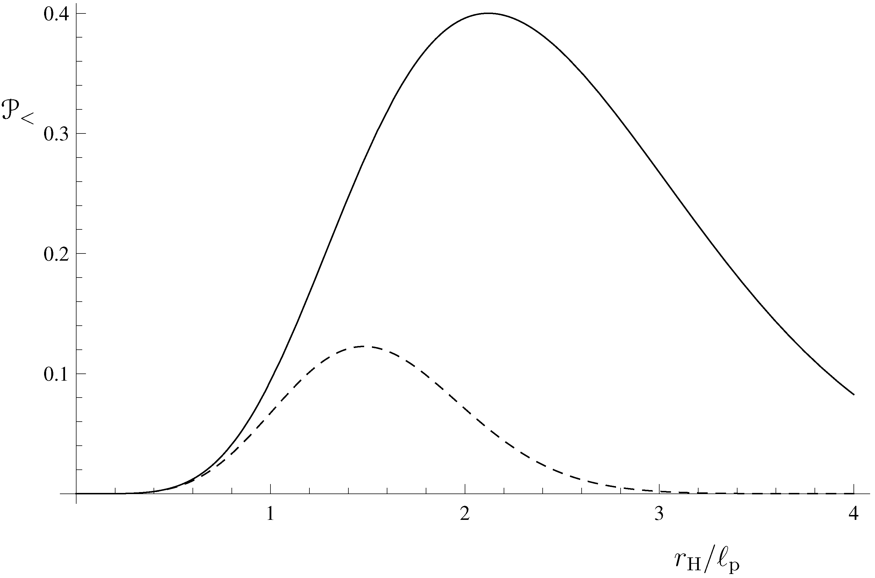
The probability density ${\mathcal{P}}_{<}$ for this particular case is represented graphically in Figure 1 for two values of the Gaussian width: $\ell ={\ell }_{\mathrm{p}}$ and $\ell =2{\ell }_{\mathrm{p}}$ (corresponding to $m=m_{\mathrm{p}}$ and $m=0.5m_{\mathrm{p}}$). As expected, larger values of the particle mass (narrower spread of the wave-packet) result in a larger probability density. By integrating the probability density, one obtains the probability $P_{\mathrm{BH}}$ for the particle to be a black hole, as stated in Equation (50). 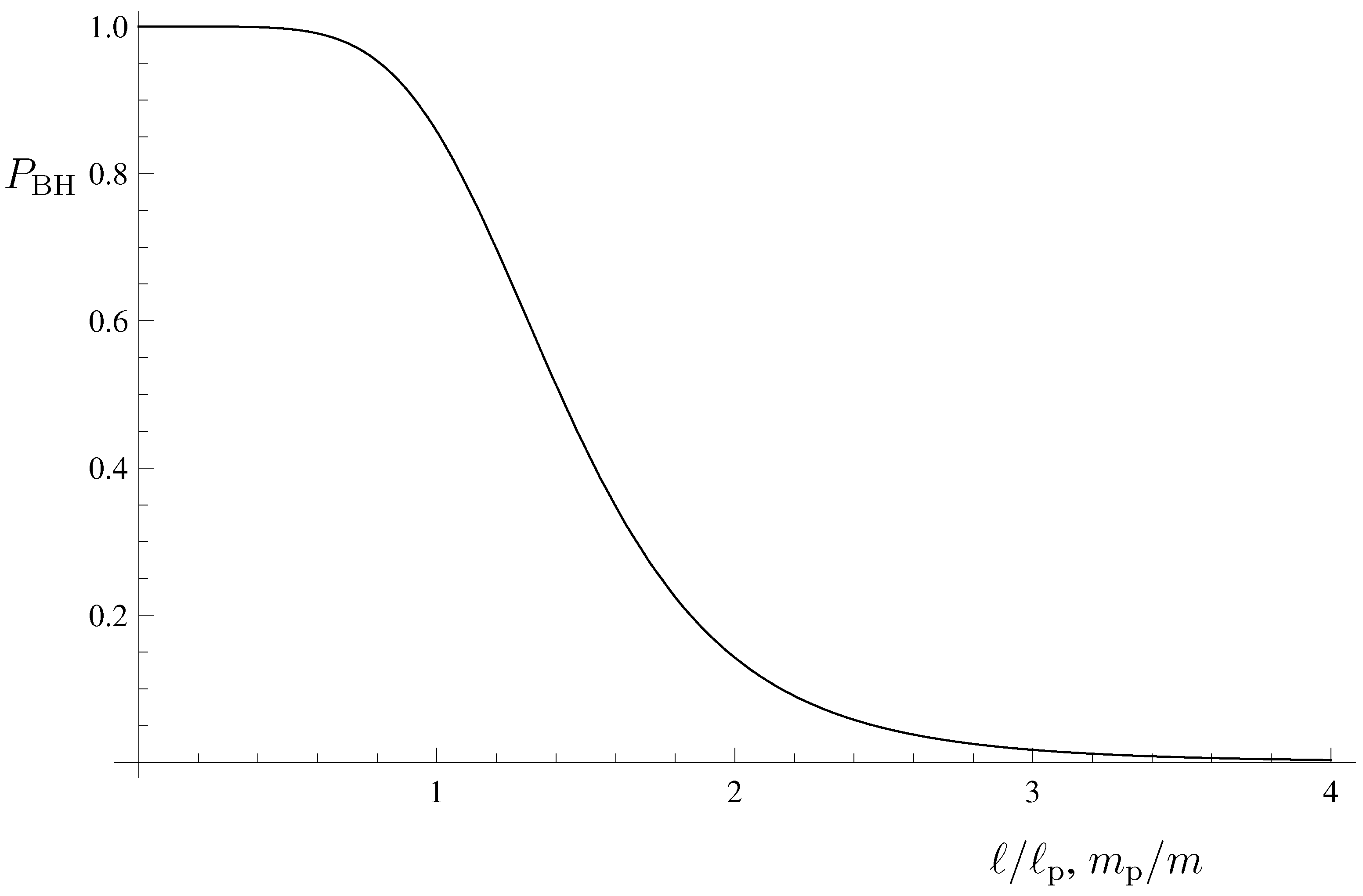Figure 2 shows $P_{\mathrm{BH}}$ as a function of ℓ (in units of ${\ell }_{\mathrm{p}}$). Gaussian wave-packets with widths below the Planck length are most likely black holes; however, this probability decreases, and it becomes negligible for widths of about $3{\ell }_{\mathrm{p}}$. The smooth transition from $P_{\mathrm{BH}}=1$ to $P_{\mathrm{BH}}=0$ in a range of mass values between $m_{\mathrm{p}}$ and $1/3m_{\mathrm{p}}$ is a feature of this quantum mechanical treatment of the horizon.

Figure 1. Probability density ${\mathcal{P}}_{<}$ in Equation (48) that a particle is inside its horizon of radius $R=r_{\mathrm{H}}$, for $\ell ={\ell }_{\mathrm{p}}$ (solid line) and for $\ell =2{\ell }_{\mathrm{p}}$ (dashed line).

Figure 1. Probability density ${\mathcal{P}}_{<}$ in Equation (48) that a particle is inside its horizon of radius $R=r_{\mathrm{H}}$, for $\ell ={\ell }_{\mathrm{p}}$ (solid line) and for $\ell =2{\ell }_{\mathrm{p}}$ (dashed line).

Figure 2. Probability $P_{\mathrm{BH}}$ in Equation (50) that a particle of width $\ell \sim m^{-1}$ is a black hole.

Figure 2. Probability $P_{\mathrm{BH}}$ in Equation (50) that a particle of width $\ell \sim m^{-1}$ is a black hole.

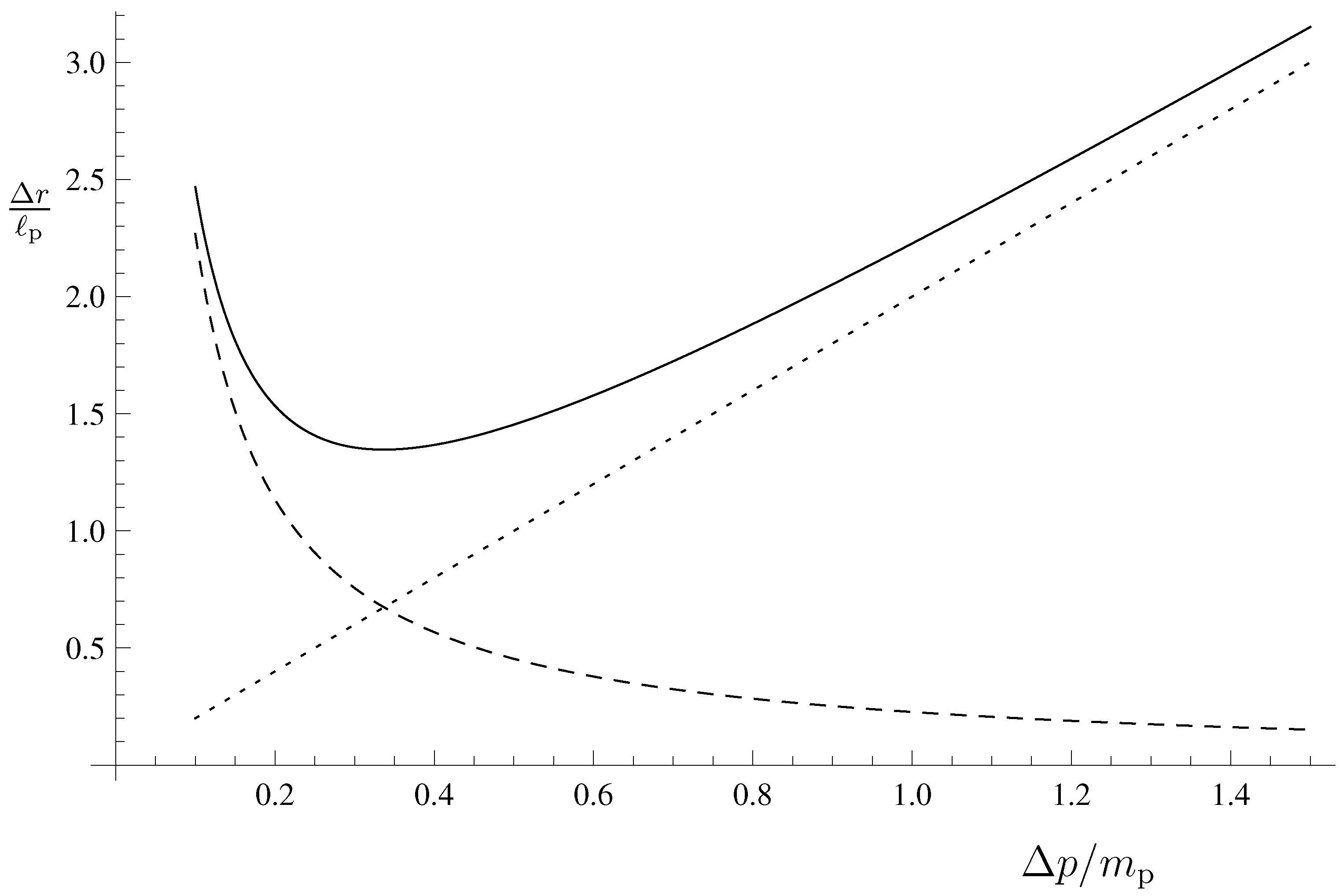
4.1. Effective GUP

It was mentioned in Section 1 that the HWF naturally leads to a GUP. For wave-packets near the Planck scale, there are two sources of uncertainty: the standard quantum mechanical uncertainty and the uncertainty in the size of the horizon radius (the complete details can be found in [24]). By linearly combining the two, we find:

$$\begin{array}{ccc}\hfill \Delta r& \equiv & \sqrt{\langle \Delta r^2\rangle }+\gamma \sqrt{\langle \Delta r_{\mathrm{H}}^2\rangle }\hfill \\ & =& \left(\frac{3\pi -8}{2\pi }\right){\ell }_{\mathrm{p}}\frac{m_{\mathrm{p}}}{\Delta p}+2\gamma {\ell }_{\mathrm{p}}\frac{\Delta p}{m_{\mathrm{p}}}\hfill \end{array}$$

(52)

where γ is a coefficient of order one. The result is plotted (for $\gamma =1$) in Figure 3, where it is also compared to the usual Heisenberg uncertainty in the position.

Figure 3. Uncertainty relation Equation (52) (solid line) as a combination of the quantum mechanical uncertainty (dashed line) and the uncertainty in the horizon radius (dotted line).

Figure 3. Uncertainty relation Equation (52) (solid line) as a combination of the quantum mechanical uncertainty (dashed line) and the uncertainty in the horizon radius (dotted line).

The uncertainty in the size of the horizon for trans-Planckian wave-packets (with masses $M\gg m_{\mathrm{p}}$) turns out to be:

$$\begin{array}{c}\hfill \Delta r_{\mathrm{H}}\sim \langle {\widehat{r}}_{\mathrm{H}}\rangle \sim R_{\mathrm{H}}\end{array}$$

(53)

Such large quantum fluctuations, with an amplitude comparable to the size of the classical gravitational radius, can hardly be considered appropriate for any classical system. Therefore, one comes to the striking conclusion that this type of source cannot represent large, semiclassical black holes, for which the relative uncertainty is expected to decrease to zero very fast for increasing mass.

5. BEC Black Hole Horizons

When analyzing the case of BEC black holes, one has to remember that these are composed of very large numbers of particles (the toy gravitons) of very small effective mass $m\ll m_{\mathrm{p}}$ (thus, very large de Broglie length, ${\lambda }_m\gg {\ell }_{\mathrm{p}}$), as opposed to the case of single massive particles studied in [24,25,26,27,28] and briefly reviewed in Section 4. According to [24], they cannot individually form (light) black holes. A generalization of the formalism to a system of N such components is possible and will allow one to show that the total energy $E=M$ is sufficient to create a proper horizon.

In order to set the notation, consider a system of N scalar particles (our “toy gravitons”), $i=1,\dots ,N$, whose dynamics is determined by a Hamiltonian $H_i$. If the particles are marginally bound according to Equation (6), the single-particle Hilbert space can be assumed to contain the discrete ground state $|m\rangle$, defined by:

$$\begin{array}{c}\hfill {\widehat{H}}_i\left|m\right.〉=m\left|m\right.〉\end{array}$$

(54)

and a gapless continuous spectrum of energy eigenstates $\left|{\omega }_i\right.〉$, such that:

$$\begin{array}{c}\hfill {\widehat{H}}_i\left|{\omega }_i\right.〉={\omega }_i\left|{\omega }_i\right.〉\end{array}$$

(55)

with ${\omega }_i>m$. The continuous spectrum reproduces the particles that escape the BEC. Each particle is then assumed to be in a state given by a superposition of $|m\rangle$ and the continuous spectrum, namely:

$$\begin{array}{c}\hfill |{\Psi }_{\mathrm{S}}^{(i)}\rangle =\frac{|m\rangle +{\gamma }_1|{\psi }_{\mathrm{S}}^{(i)}\rangle }{\sqrt{1+{\gamma }_1^2}}\end{array}$$

(56)

where ${\gamma }_1\in {\mathbb{R}}_{+}$ is a dimensionless parameter that weights the relative probability amplitude for each “toy graviton” to be in the continuum rather than the ground state. The total wave-function will be given by the symmetrized product of N such states,

$$\begin{array}{c}\hfill |{\Psi }_N\rangle \simeq \frac{1}{N!}\sum _{\{{\sigma }_i\}}^N\left[\underset{i=1}{\overset{N}{⨂}}|{\Psi }_{\mathrm{S}}^{(i)}\rangle \right]\end{array}$$

(57)

where the sum is over all of the permutations $\{{\sigma }_i\}$ of the N excitations. Since the interaction is included in terms proportional to powers of ${\gamma }_1$, the spectral decomposition of this N-particle state can be obtained by defining the total Hamiltonian simply as the sum of N single-particle Hamiltonians,

$$\begin{array}{c}\hfill \widehat{H}=\underset{i=1}{\overset{N}{⨁}}{\widehat{H}}_i\end{array}$$

(58)

The corresponding eigenvector for the discrete ground state with $M=Nm$ is given by:

$$\begin{array}{c}\hfill \widehat{H}\left|M\right.〉=M\left|M\right.〉\end{array}$$

(59)

and the eigenvectors for the continuum by:

$$\begin{array}{c}\hfill \widehat{H}\left|E\right.〉=E\left|E\right.〉\end{array}$$

(60)

The spectral coefficients are computed by projecting $|{\Psi }_{\mathrm{N}}\rangle$ on these eigenvectors.

5.1. Black Holes with No Hair

The highly idealized case in Equation (40) admits precisely one mode, given by:

$$\begin{array}{c}\hfill k_{\mathrm{c}}=\frac{\pi }{R_{\mathrm{H}}}=\frac{\pi }{2\sqrt{N}{\ell }_{\mathrm{p}}}\end{array}$$

(61)

so that, on the surface of the black hole, ${\varphi }_{k_{\mathrm{c}}}(R_{\mathrm{H}})\simeq j_0(k_{\mathrm{c}}{R}_{\mathrm{H}})=0$, and the scalar field vanishes outside of $r=R_{\mathrm{H}}$,

$$\begin{array}{c}\hfill {\psi }_{\mathrm{S}}(r_i)=\langle r_i\mid k_{\mathrm{c}}\rangle =\left\{\begin{array}{cc}{\mathcal{N}}_{\mathrm{c}}{j}_0(k_{\mathrm{c}}{r}_i)\hfill & \mathrm{for}r<R_{\mathrm{H}}\hfill \\ \\ 0\hfill & \mathrm{for}r>R_{\mathrm{H}}\hfill \end{array}\right.\end{array}$$

(62)

where ${\mathcal{N}}_{\mathrm{c}}=\sqrt{\pi /2R_{\mathrm{H}}^3}$ is a normalization factor such that:

$$\begin{array}{c}\hfill 4\pi {\mathcal{N}}_{\mathrm{c}}^2{\int }_0^{R_{\mathrm{H}}}{|j_0(k_{\mathrm{c}}r)|}^2{r}^2\mathrm{d}r=1\end{array}$$

(63)

This approximate mode is plotted in Figure 4 and compared to a Gaussian distribution of the kind considered in [58].

Figure 4. Scalar field mode of momentum number $k_{\mathrm{c}}$: ideal approximation in Equation (62) (thick solid line) compared to exact $j_0(k_{\mathrm{c}}r)$ (dashed line). The thin solid line represents a Gaussian distribution of the kind considered in [58].

Figure 4. Scalar field mode of momentum number $k_{\mathrm{c}}$: ideal approximation in Equation (62) (thick solid line) compared to exact $j_0(k_{\mathrm{c}}r)$ (dashed line). The thin solid line represents a Gaussian distribution of the kind considered in [58].

It was noted before the end of Section 3.1 that a scalar field that vanishes everywhere outside $r=R_{\mathrm{H}}$ is inconsistent with the existence of an outer Newtonian potential, but one can still investigate the case for the sake of having a complete picture. A system of N such modes will be described by a wave-function, which is the (totally symmetrized) product of $N\sim M^2$ equal modes and ${\gamma }_1=0$, that is:

$$\begin{array}{c}\hfill {\Psi }_{\mathrm{N}}(r_1,\dots ,r_N)=\frac{{\mathcal{N}}_{\mathrm{c}}^N}{N!}\sum _{\{{\sigma }_i\}}^N\prod _{i=1}^N{j}_0(k_{\mathrm{c}}{r}_i)\end{array}$$

(64)

This is clearly an eigenstate of the total Hamiltonian:

$$\begin{array}{c}\hfill \widehat{H}|{\Psi }_{\mathrm{N}}\rangle =N\hslash k_{\mathrm{c}}|{\Psi }_{\mathrm{N}}\rangle =M|{\Psi }_{\mathrm{N}}\rangle \end{array}$$

(65)

and there exists only one non-vanishing coefficient in the spectral decomposition: $C(E)=1$, for $E=N\hslash k_{\mathrm{c}}=M$, corresponding to a probability density for finding the horizon size between $r_{\mathrm{H}}$ and $r_{\mathrm{H}}+\mathrm{d}{r}_{\mathrm{H}}$:

$$\begin{array}{ccc}\hfill {\mathcal{P}}_{\mathrm{H}}(r_{\mathrm{H}})& =& 4\pi r_{\mathrm{H}}^2{\left|{\psi }_{\mathrm{H}}(r_{\mathrm{H}})\right|}^2\hfill \\ & =& \delta (r_{\mathrm{H}}-R_{\mathrm{H}})\hfill \end{array}$$

(66)

This result, and the fact that all of the excitations in the mode $k_{\mathrm{c}}$ are confined within the radius $R_{\mathrm{H}}\simeq {\lambda }_{\mathrm{c}}$, leads to the conclusion that the system is a black hole,

$$\begin{array}{ccc}\hfill P_{\mathrm{BH}}& \simeq & 4\pi {\mathcal{N}}_{\mathrm{c}}^2{\int }_0^{\infty }\mathrm{d}{r}_{\mathrm{H}}\delta (r_{\mathrm{H}}-R_{\mathrm{H}}){\int }_0^{r_{\mathrm{H}}}{|j_0(k_{\mathrm{c}}r)|}^2{r}^2\mathrm{d}r\hfill \\ & =& P_{\mathrm{S}}(r<R_{\mathrm{H}})=1\hfill \end{array}$$

(67)

with the horizon located at its classical radius,

$$\begin{array}{c}\hfill \langle {\widehat{r}}_{\mathrm{H}}\rangle \equiv \langle {\psi }_{\mathrm{H}}|{\widehat{r}}_{\mathrm{H}}|{\psi }_{\mathrm{H}}\rangle =R_{\mathrm{H}}\end{array}$$

(68)

and with absolutely negligible uncertainty:

$$\begin{array}{c}\hfill \Delta r_{\mathrm{H}}^2\equiv \langle {\psi }_{\mathrm{H}}|\left({\widehat{r}}_{\mathrm{H}}^2-R_{\mathrm{H}}^2\right)|{\psi }_{\mathrm{H}}\rangle \simeq 0\end{array}$$

(69)

The sharply vanishing uncertainty in $\langle {\widehat{r}}_{\mathrm{H}}\rangle$ is an unphysical result, which is a consequence of considering the macroscopic black hole as a pure quantum mechanical state built by superposing many wave-functions of the type Equation (62). Furthermore, a zero field at $r>R_{\mathrm{H}}$ cannot reproduce the Newtonian potential outside the black hole, which clearly contradicts observations.

For a more realistic macroscopic black hole (with $N\gg 1$), one therefore needs to consider the existence of more modes besides the ones with $k=k_{\mathrm{c}}$. In this case, the modes with $k=k_{\mathrm{c}}$ form a discrete spectrum (which comes from $k_{\mathrm{c}}$ being the minimum allowed momentum, in agreement with the idea of a BEC of gravitons), and must be treated separately. If modes with $k>k_{\mathrm{c}}$ exist, these would not be (marginally) trapped and could “leak out”, thus representing a simple modelization of the Hawking flux. They will form a continuous spectrum, which will lead to fuzziness in the horizon’s location. The precise form of this part of the spectrum is however an open issue, and we will review several possibilities in the next sections.

5.2. Black Hole with Gaussian Excited Spectrum

Let us start assuming a continuous distribution in momentum space of each of the N scalar states given by half a Gaussian peaked around $k_{\mathrm{c}}$ (Figure 5 displays a few modes above $k_{\mathrm{c}}$),

$$\begin{array}{c}\hfill |{\psi }_{\mathrm{S}}^{(i)}\rangle ={\mathcal{N}}_{\gamma }\left(|k_{\mathrm{c}}\rangle +{\gamma }_1{\int }_{k_{\mathrm{c}}}^{\infty }\frac{\sqrt{2}\mathrm{d}{k}_i}{\sqrt{{\Delta }_i\sqrt{\pi }}}{e}^{-\frac{{\hslash }^2{(k_i-k_{\mathrm{c}})}^2}{2{\Delta }_i^2}}|k_i\rangle \right)\end{array}$$

(70)

where $i=1,\dots ,N$, the ket $|k\rangle$ denotes the eigenmode of eigenvalue k, and:

$$\begin{array}{c}\hfill {\mathcal{N}}_{\gamma }={\left(1+{\gamma }_1^2\right)}^{-1/2}\end{array}$$

(71)

is a normalization factor. Furthermore, the width of the Gaussians is ${\Delta }_i=m\simeq M/N\simeq m_{\mathrm{p}}/\sqrt{N}$, as calculated from the typical mode spatial size $k_{\mathrm{c}}^{-1}\sim \sqrt{N}{\ell }_{\mathrm{p}}$, and is the same for all particles. This is, of course, a necessary simplification needed in order to simplify the calculations (more generally, one could assume a different width for each mode $k_i$). Since $m=\hslash k_{\mathrm{c}}$ and $E_i=\hslash k_i$, one can also write:

$$\begin{array}{c}\hfill |{\psi }_{\mathrm{S}}^{(i)}\rangle ={\mathcal{N}}_{\gamma }\left(|m\rangle +{\gamma }_1{\int }_m^{\infty }\frac{\sqrt{2}\mathrm{d}{E}_i}{\sqrt{m\sqrt{\pi }}}{e}^{-\frac{{(E_i-m)}^2}{2m^2}}|E_i\rangle \right)\end{array}$$

(72)

The total wave-function will be given by the symmetrized product of N such states and can be written by grouping equal powers of ${\gamma }_1$ as follows:

$$\begin{array}{ccc}\hfill |{\Psi }_{\mathrm{N}}\rangle & \simeq & \frac{1}{N!}\sum _{\{{\sigma }_i\}}^N\left[\underset{i=1}{\overset{N}{⨂}}|m\rangle \right]\hfill \\ & & +\frac{{\gamma }_1}{N!}{\left(\frac{2}{m\sqrt{\pi }}\right)}^{1/2}\sum _{\{{\sigma }_i\}}^N\left[\underset{i=2}{\overset{N}{⨂}}|m\rangle \otimes {\int }_m^{\infty }\mathrm{d}{E}_1{e}^{-\frac{{(E_1-m)}^2}{2m^2}}|E_1\rangle \right]\hfill \\ & & +\frac{{\gamma }_1^2}{N!}\left(\frac{2}{m\sqrt{\pi }}\right)\sum _{\{{\sigma }_i\}}^N\left[\underset{i=3}{\overset{N}{⨂}}|m\rangle \otimes {\int }_m^{\infty }\mathrm{d}{E}_1{e}^{-\frac{{(E_1-m)}^2}{2m^2}}|E_1\rangle \otimes {\int }_m^{\infty }\mathrm{d}{E}_2{e}^{-\frac{{(E_2-m)}^2}{2m^2}}|E_2\rangle \right]\hfill \\ & & +\dots \hfill \\ & & +\frac{{\gamma }_1^J}{N!}{\left(\frac{2}{m\sqrt{\pi }}\right)}^{J/2}\sum _{\{{\sigma }_i\}}^N\left[\underset{i=J+1}{\overset{N}{⨂}}|m\rangle \underset{j=1}{\overset{J}{⨂}}{\int }_m^{\infty }\mathrm{d}{E}_j{e}^{-\frac{{(E_j-m)}^2}{2m^2}}|E_j\rangle \right]\hfill \\ & & +\dots \hfill \\ & & +\frac{{\gamma }_1^N}{N!}{\left(\frac{2}{m\sqrt{\pi }}\right)}^{N/2}\sum _{\{{\sigma }_i\}}^N\left[\underset{i=1}{\overset{N}{⨂}}{\int }_m^{\infty }\mathrm{d}{E}_i{e}^{-\frac{{(E_i-m)}^2}{2m^2}}|E_i\rangle \right]\hfill \end{array}$$

(73)

where the power of ${\gamma }_1$ clearly equals the number of bosons in an “excited” mode with $k>k_{\mathrm{c}}$. One can then identify two regimes, depending on the value of ${\gamma }_1$ (for further details, readers are directed to Appendix A in [35]).

Figure 5. Modes of momentum number $k=k_{\mathrm{c}}$ (thick solid line), $k=(5/4)k_{\mathrm{c}}$ (dashed line), $k=(3/2)k_{\mathrm{c}}$ (dotted line), $k=(7/4)k_{\mathrm{c}}$ (dash-dotted line) and $k=2k_{\mathrm{c}}$ (thin solid line). The relative weight is determined according to Equation (70).

Figure 5. Modes of momentum number $k=k_{\mathrm{c}}$ (thick solid line), $k=(5/4)k_{\mathrm{c}}$ (dashed line), $k=(3/2)k_{\mathrm{c}}$ (dotted line), $k=(7/4)k_{\mathrm{c}}$ (dash-dotted line) and $k=2k_{\mathrm{c}}$ (thin solid line). The relative weight is determined according to Equation (70).

For ${\gamma }_1\ll 1$, to leading order in ${\gamma }_1$, the spectral coefficient for $E\ge M$ is given by the term corresponding to just one particle in the continuum,

$$\begin{array}{c}\hfill C(E\ge M)\simeq {\mathcal{N}}_{\gamma }\left[{\delta }_{E,M}+{\gamma }_1{\left(\frac{2}{m\sqrt{\pi }}\right)}^{1/2}{e}^{-\frac{{(E-M)}^2}{2m^2}}\right]\end{array}$$

(74)

where ${\delta }_{A,B}$ is a Kronecker delta for the discrete part of the spectrum. The width $m\sim m_{\mathrm{p}}/\sqrt{N}$ is the typical energy of Hawking quanta emitted by a black hole of mass $M\simeq \sqrt{N}{m}_{\mathrm{p}}$. The expectation value of the energy to next-to-leading order for large N and small ${\gamma }_1$ is:

$$\begin{array}{ccc}\hfill \langle E\rangle & \simeq & {\mathcal{N}}_{\gamma }^2\left(M+{\int }_M^{\infty }E{C}^2(E)\mathrm{d}E\right)\hfill \\ & \simeq & \sqrt{N}{m}_{\mathrm{p}}\left(1+\frac{{\gamma }_1^2/\sqrt{\pi }}{1+{\gamma }_1^2}\frac{1}{N}\right)\hfill \\ & \simeq & \sqrt{N}{m}_{\mathrm{p}}\left(1+\frac{{\gamma }_1^2}{\sqrt{\pi }N}\right)\hfill \end{array}$$

(75)

and its uncertainty:

$$\begin{array}{c}\hfill \Delta E=\sqrt{\langle E^2\rangle -{\langle E\rangle }^2}\simeq \frac{{\gamma }_1{m}_{\mathrm{p}}}{\sqrt{2N}}\end{array}$$

(76)

One can also calculate the ratio:

$$\begin{array}{c}\hfill \frac{\Delta E}{\langle E\rangle }\simeq \frac{{\gamma }_1}{\sqrt{2}N}\end{array}$$

(77)

where only the leading order in the large N expansion was kept. From the expression of the Schwarzschild radius $r_{\mathrm{H}}=2{\ell }_{\mathrm{p}}E/m_{\mathrm{p}}$, one easily finds $\langle {\widehat{r}}_{\mathrm{H}}\rangle \simeq R_{\mathrm{H}}$, with $R_{\mathrm{H}}$ given in Equation (39), and:

$$\begin{array}{c}\hfill \frac{\Delta r_{\mathrm{H}}}{\langle {\widehat{r}}_{\mathrm{H}}\rangle }\sim \frac{1}{N}\end{array}$$

(78)

which vanishes rapidly for large N. This case describes a macroscopic BEC black hole with (very) little quantum hair, in agreement with [16,17,18,19,20,21,22], thus overcoming the problem of the large fluctuations Equation (53), which appear in the case of a single massive particle.

This “hair” is expected to represent the Hawking radiation field, and the connection with the thermal Hawking radiation will become more clear in Section 5.4, where a different form of the continuous spectrum will be employed

5.3. Quantum Hair with No Black Hole

When ${\gamma }_1\gtrsim 1$ and $N\gg 1$, all of the N particles are in the continuum, while the ground state ${\varphi }_{k_{\mathrm{c}}}$ is totally depleted. The coefficient ${\gamma }_1^N$ and any overall factors can be omitted in this case, and one finds:

$$\begin{array}{c}\hfill C(E\ge M)\simeq {\int }_m^{\infty }\mathrm{d}{E}_1\cdots {\int }_m^{\infty }\mathrm{d}{E}_{N}exp\left\{-\sum _{i=1}^N\frac{{(E_i-m)}^2}{2m^2}\right\}\delta \left(E-\sum _{i=1}^N{E}_i\right)\end{array}$$

(79)

along with $C(E<M)\simeq 0$. Note that, in this case, the mass $M=Nm$ still represents the minimum energy of the system corresponding to the “ideal” black hole with all of the N particles in the ground state $|k_{\mathrm{c}}\rangle$. For $N=M/m\gg 1$, this spectral function is estimated analytically in [35] and is given by:

$$\begin{array}{c}\hfill C(E\ge M)\simeq \sqrt{\frac{2}{\pi m^3}}(E-M)e^{-\frac{{(E-M)}^2}{4m^2}}\end{array}$$

(80)

which is peaked slightly above $E\simeq M=Nm$, with a width $\sqrt{2}{\Delta }_i\sim m$, so that the (normalized) expectation value:

$$\begin{array}{c}\hfill \langle E\rangle \simeq {\int }_M^{\infty }E{C}^2(E)\mathrm{d}E=M+2\sqrt{\frac{2}{\pi }}m\end{array}$$

(81)

consistently for a system built out of continuous modes. To be in the continuous part of the spectrum, the energy of these modes must be (slightly) larger than m. For $N\gg 1$, however, $\langle E\rangle =M[1+\mathcal{O}(N^{-1})]$, and the energy quickly approaches the minimum value M. This is also confirmed by the uncertainty:

$$\begin{array}{c}\hfill \Delta E\simeq \sqrt{\frac{3\pi -8}{\pi }}m\end{array}$$

(82)

or $\Delta E\sim N^{-1/2}$.

The corresponding horizon wave-function is obtained by using $r_{\mathrm{H}}=2{\ell }_{\mathrm{p}}E/m_{\mathrm{p}}$, and is approximately given by:

$$\begin{array}{c}\hfill {\psi }_{\mathrm{H}}(r_{\mathrm{H}}\ge 2\sqrt{N}{\ell }_{\mathrm{p}})\simeq \left(r_{\mathrm{H}}-2\sqrt{N}{\ell }_{\mathrm{p}}\right)e^{-\frac{{\left(r_{\mathrm{H}}-2\sqrt{N}{\ell }_{\mathrm{p}}\right)}^2}{16{\ell }_{\mathrm{p}}^2/N}}\end{array}$$

(83)

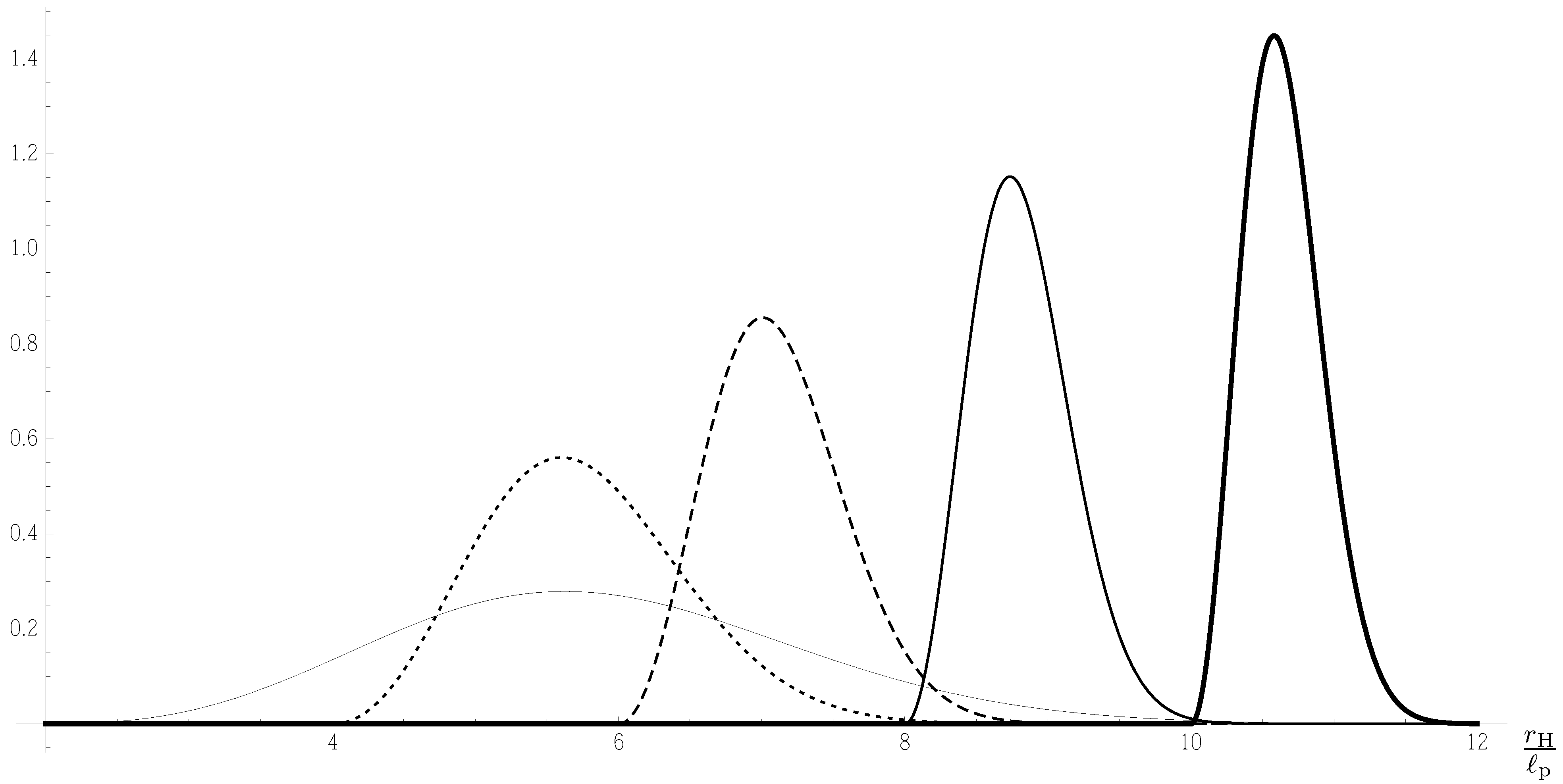
and ${\psi }_{\mathrm{H}}(r_{\mathrm{H}}<2\sqrt{N}{\ell }_{\mathrm{p}})\simeq 0$. The probability density of finding the gravitational radius between $r_{\mathrm{H}}$ and $r_{\mathrm{H}}+\mathrm{d}{r}_{\mathrm{H}}$ is plotted in Figure 6 for different values of N. The plot shows that for $N\sim 1$, the uncertainty in the size of the gravitational radius is large, but it decreases very fast with increasing N. The expectation value:

$$\begin{array}{c}\hfill \langle {\widehat{r}}_{\mathrm{H}}\rangle \simeq 2\sqrt{N}{\ell }_{\mathrm{p}}\left(1+\sqrt{\frac{2}{\pi }}\frac{2}{N}\right)=R_{\mathrm{H}}\left[1+\mathcal{O}(N^{-1})\right]\end{array}$$

(84)

approaches (from above) the horizon radius of the ideal black hole, $R_{\mathrm{H}}=2\sqrt{N}{\ell }_{\mathrm{p}}$, for large N. Since $\langle {\widehat{r}}_{\mathrm{H}}\rangle >R_{\mathrm{H}}$, one can safely view it as a trapping surface, whose uncertainty is proportional to the energy $m=m_{\mathrm{p}}/\sqrt{N}$, that is:

$$\begin{array}{c}\hfill \frac{\Delta r_{\mathrm{H}}}{\langle {\widehat{r}}_{\mathrm{H}}\rangle }=\frac{\sqrt{\langle {\widehat{r}}_{\mathrm{H}}^2-{\langle {\widehat{r}}_{\mathrm{H}}\rangle }^2\rangle }}{\langle {\widehat{r}}_{\mathrm{H}}\rangle }\simeq \frac{1}{N}\end{array}$$

(85)

which vanishes as fast as in the previous case for large N. This is also expected in a proper semiclassical regime [16,17,18,19,20,21,22].

It needs to be emphasized that cases with ${\gamma }_1\ll ̸1$ do not describe a BEC black hole, because most or all of the gravitons are in some excited mode with $k>k_{\mathrm{c}}$. However, one can think that these states may play a role either at the threshold of black hole formation (before the gravitons condense into the ground state $|k_{\mathrm{c}}\rangle$ and form a BEC) or near the end of black hole evaporation.

Figure 6. Probability density for the gravitational radius $r_{\mathrm{H}}$ for $N=1$ ($R_{\mathrm{H}}=2{\ell }_{\mathrm{p}}$; thin solid line), $N=4$ ($R_{\mathrm{H}}=4{\ell }_{\mathrm{p}}$; dotted line), $N=9$ ($R_{\mathrm{H}}=6{\ell }_{\mathrm{p}}$; dashed line), $N=16$ ($R_{\mathrm{H}}=8{\ell }_{\mathrm{p}}$; solid line) and $N=25$ ($R_{\mathrm{H}}=10{\ell }_{\mathrm{p}}$; thick solid line). The curves clearly become narrower the larger N.

Figure 6. Probability density for the gravitational radius $r_{\mathrm{H}}$ for $N=1$ ($R_{\mathrm{H}}=2{\ell }_{\mathrm{p}}$; thin solid line), $N=4$ ($R_{\mathrm{H}}=4{\ell }_{\mathrm{p}}$; dotted line), $N=9$ ($R_{\mathrm{H}}=6{\ell }_{\mathrm{p}}$; dashed line), $N=16$ ($R_{\mathrm{H}}=8{\ell }_{\mathrm{p}}$; solid line) and $N=25$ ($R_{\mathrm{H}}=10{\ell }_{\mathrm{p}}$; thick solid line). The curves clearly become narrower the larger N.

5.4. BEC with Thermal Quantum Hair

In Section 5.2, it was shown that, for ${\gamma }_1\ll 1$, the quantum state of N scalars is dominated by the configurations with just one boson in the continuum of excited states, while the remaining $N-1$ gravitons form the BEC. A Gaussian distribution was used to describe the continuous part of the spectrum, and it was found that the spectral function has a typical width of the order of the Hawking temperature,

$$\begin{array}{c}\hfill T_{\mathrm{H}}=\frac{m_{\mathrm{p}}^2}{4\pi M}\simeq \frac{m_{\mathrm{p}}}{\sqrt{N}}\end{array}$$

(86)

or $T_{\mathrm{H}}\simeq m$. It is thus logical to ask what happens if the Gaussian distribution in Equation (70) is replaced by a thermal spectrum at the temperature $T_{\mathrm{H}}$.

We hence start with a Planckian distribution (using a Boltzmann distribution for $N=1$ is also possible; however, for $N>1$, it is affected by IR divergences) at the temperature $T_{\mathrm{H}}=m$ for the continuum part, namely:

$$\begin{array}{ccc}\hfill |{\psi }_{\mathrm{S}}^{(i)}\rangle & =& \frac{{\mathcal{N}}_{\mathrm{H}}}{m^{3/2}}{\int }_m^{\infty }\mathrm{d}{\omega }_i\frac{({\omega }_i-m)}{exp\left\{\frac{{\omega }_i-m}{m}\right\}-1}\left|{\omega }_i\right.〉\hfill \\ & \equiv & {\mathcal{N}}_{\mathrm{H}}{\int }_0^{\infty }\mathrm{d}{\mathcal{E}}_{i}G({\mathcal{E}}_i)|{\mathcal{E}}_i\rangle \hfill \end{array}$$

(87)

where ${\mathcal{N}}_{\mathrm{H}}=\sqrt{3}/\sqrt{{\pi }^2-6\zeta (3)}\simeq 1.06$, the dimensionless variables:

$$\begin{array}{c}\hfill {\mathcal{E}}_i=\frac{{\omega }_i-m}{m}\end{array}$$

(88)

and the states $|{\mathcal{E}}_i\rangle =m^{1/2}|{\omega }_i\rangle$ were introduced, such that the identity in the continuum can be written as:

$$\begin{array}{c}\hfill {\int }_0^{\infty }\mathrm{d}{\mathcal{E}}_i|{\mathcal{E}}_i\rangle \langle {\mathcal{E}}_i|={\int }_m^{\infty }\mathrm{d}{\omega }_i|{\omega }_i\rangle \langle {\omega }_i|=\mathbb{I}\end{array}$$

(89)

The “thermal hair” is again assumed to appear due to the scatterings between the scalars inside the BEC; therefore, the parameter ${\gamma }_1$ should be related to the toy gravitons’ self-coupling α. In this exercise, it is however kept as a free variable, so that one could relate it a posteriori to known features of the Hawking radiation.

Assuming that ${\gamma }_1\ne 0$ yields a good enough approximation of the leading effects due to these bosons’ self-interactions, the BEC can be treated as being made of otherwise free scalars. The total wave-function of the system of N such bosons can again be written by collecting powers of ${\gamma }_1$,

$$\begin{array}{ccc}\hfill |{\Psi }_N\rangle & \simeq & \frac{1}{N!}\sum _{\{{\sigma }_i\}}^N\left[\underset{i=1}{\overset{N}{⨂}}|m\rangle \right]\hfill \\ & & +{\gamma }_1\frac{{\mathcal{N}}_{\mathrm{H}}}{N!}\sum _{\{{\sigma }_i\}}^N\left[\underset{i=2}{\overset{N}{⨂}}|m\rangle \otimes {\int }_0^{\infty }\mathrm{d}{\mathcal{E}}_{1}G({\mathcal{E}}_1)|{\mathcal{E}}_1\rangle \right]\hfill \\ & & +{\gamma }_1^2\frac{{\mathcal{N}}_{\mathrm{H}}^2}{N!}\sum _{\{{\sigma }_i\}}^N\left[\underset{i=3}{\overset{N}{⨂}}|m\rangle \otimes {\int }_0^{\infty }\mathrm{d}{\mathcal{E}}_{1}G({\mathcal{E}}_1)|{\mathcal{E}}_1\rangle \otimes {\int }_0^{\infty }\mathrm{d}{\mathcal{E}}_{2}G({\mathcal{E}}_2)|{\mathcal{E}}_2\rangle \right]\hfill \\ & & +\dots \hfill \\ & & +{\gamma }_1^J\frac{{\mathcal{N}}_{\mathrm{H}}^J}{N!}\sum _{\{{\sigma }_i\}}^N\left[\underset{i=J+1}{\overset{N}{⨂}}|m\rangle \underset{j=1}{\overset{J}{⨂}}{\int }_0^{\infty }\mathrm{d}{\mathcal{E}}_{j}G({\mathcal{E}}_j)|{\mathcal{E}}_j\rangle \right]\hfill \\ & & +\dots \hfill \\ & & +{\gamma }_1^N\frac{{\mathcal{N}}_{\mathrm{H}}^N}{N!}\sum _{\{{\sigma }_i\}}^N\left[\underset{i=1}{\overset{N}{⨂}}{\int }_0^{\infty }\mathrm{d}{\mathcal{E}}_{i}G({\mathcal{E}}_i)|{\mathcal{E}}_i\rangle \right]\hfill \end{array}$$

(90)

where the overall normalization constant of $1/{(1+{\gamma }_1^2)}^{N/2}$ was omitted for the sake of simplicity.

For $E=M=Nm$, on neglecting an overall normalization factor, one obviously has:

$$\begin{array}{c}\hfill C(M)\simeq \frac{1}{N!}\langle M|\sum _{\{{\sigma }_i\}}^N\left[\underset{i=1}{\overset{N}{⨂}}|m\rangle \right]=1\end{array}$$

(91)

For energies above the ground state, $E>M=Nm$, the spectral coefficients are given by:

$$\begin{array}{c}\hfill C(E>M)=\langle E\mid {\Psi }_N\rangle \end{array}$$

(92)

and using the dimensionless variables Equation (88), along with:

$$\begin{array}{c}\hfill \mathcal{E}=\frac{E-M}{m}\end{array}$$

(93)

one finds:

$$\begin{array}{ccc}\hfill C(\mathcal{E}>0)& \simeq & {\gamma }_1{\mathcal{N}}_{\mathrm{H}}G(\mathcal{E})\hfill \\ & & +{\gamma }_1^2{\mathcal{N}}_{\mathrm{H}}^2{\int }_0^{\infty }G({\mathcal{E}}_1)G(\mathcal{E}-{\mathcal{E}}_1)\mathrm{d}{\mathcal{E}}_1\hfill \\ & & +\dots \hfill \\ & & +{\gamma }_1^N{\mathcal{N}}_{\mathrm{H}}^N{\int }_0^{\infty }G({\mathcal{E}}_1)\mathrm{d}{\mathcal{E}}_1\times \cdots \times {\int }_0^{\infty }G({\mathcal{E}}_N)\mathrm{d}{\mathcal{E}}_N\delta \left(\mathcal{E}-\sum _{i=1}^N{\mathcal{E}}_i\right)\hfill \\ & \equiv & \sum _{n=1}^N{\gamma }_1^n{C}_n(\mathcal{E})\hfill \end{array}$$

(94)

where all of the coefficients in this expression can be written as:

$$\begin{array}{c}\hfill C_n={\mathcal{N}}_{\mathrm{H}}^n{\int }_0^{\infty }G({\mathcal{E}}_1)\mathrm{d}{\mathcal{E}}_1\times \cdots \times {\int }_0^{\infty }G({\mathcal{E}}_{n-1})\mathrm{d}{\mathcal{E}}_{n-1}G\left(\mathcal{E}-\sum _{i=1}^{n-1}{\mathcal{E}}_i\right)\end{array}$$

(95)

Each integral in ${\mathcal{E}}_i$ is peaked around ${\mathcal{E}}_i=0$, so that one can approximate:

$$\begin{array}{c}\hfill G\left(\mathcal{E}-\sum _{i=1}^{n-1}{\mathcal{E}}_i\right)=\frac{\mathcal{E}-{\sum }_{i=1}^{n-1}{\mathcal{E}}_i}{exp\left\{\mathcal{E}-{\sum }_{i=1}^{n-1}{\mathcal{E}}_i\right\}-1}\simeq \frac{\mathcal{E}}{exp\left\{\mathcal{E}\right\}-1}=G(\mathcal{E})\end{array}$$

(96)

for $2\le n\le N$. Therefore:

$$\begin{array}{ccc}\hfill C_n& \simeq & {\mathcal{N}}_{\mathrm{H}}{\left({\mathcal{N}}_{\mathrm{H}}\frac{{\pi }^2}{6}\right)}^{n-1}G(\mathcal{E})={(1.75)}^{n-1}{\mathcal{N}}_{\mathrm{H}}G(\mathcal{E})\hfill \end{array}$$

(97)

Upon rescaling:

$$\begin{array}{c}\hfill \gamma \simeq 0.57\sum _{j=1}^N{\left(1.75{\gamma }_1\right)}^j\end{array}$$

(98)

and switching back to dimensionful variables, one finds:

$$\begin{array}{ccc}\hfill C(E>M)& \simeq & \gamma \frac{{\mathcal{N}}_{\mathrm{H}}}{\sqrt{m}}\frac{(E-M)/m}{exp\left\{(E-M)/m\right\}-1}\hfill \end{array}$$

(99)

This approximation was checked numerically to work extremely well for a wide range of N. The details of the numerical analysis can be found in Appendix B of [35].

The result in Equation (99) means that one can describe the quantum state of the N-particle system as the (normalized) single-particle state:

$$\begin{array}{c}\hfill |{\Psi }_{\mathrm{S}}\rangle \simeq \frac{|M\rangle +\gamma |\psi \rangle }{\sqrt{1+{\gamma }^2}}\end{array}$$

(100)

where:

$$\begin{array}{c}\hfill |\psi \rangle =\frac{{\mathcal{N}}_{\mathrm{H}}}{\sqrt{m}}\frac{(E-M)/m}{\exp \left\{(E-M)/m\right\}-1}|E\rangle \end{array}$$

(101)

Therefore, the BEC black hole effectively looks like one particle of very large mass $M=Nm$ in a superposition of states with “Planckian hair”. To have most of the toy gravitons in the ground state, all that needs to be assumed is $\gamma \ll 1$. However, nothing prevents one from also considering the above approximate wave-function for $\gamma \simeq 1$ or even larger.

5.4.1. Partition Function and Entropy

It is now straightforward to employ the effective wave-function Equation (100) to compute expectations values, such as:

$$\begin{array}{ccc}\hfill \langle \widehat{H}\rangle & =& \frac{1}{1+{\gamma }^2}\left\{M+{\gamma }^2\frac{{\mathcal{N}}_{\mathrm{H}}^2}{m}{\int }_M^{\infty }{\left[\frac{(E-M)/m}{\exp \left\{(E-M)/m\right\}-1}\right]}^{2}E\mathrm{d}E\right\}\hfill \\ \hfill & =& m_{\mathrm{p}}\sqrt{N}\left[1+{\gamma }^2\frac{{\mathcal{N}}_{\mathrm{H}}^2}{N}\left(6\zeta (3)-\frac{{\pi }^4}{15}\right)\right]+O({\gamma }^4)\hfill \end{array}$$

(102)

where the higher powers of the parameter γ were discarded and the approximation ${(1+{\gamma }^2)}^{-1}\simeq 1-{\gamma }^2$ was used.

Since:

$$\begin{array}{ccc}\hfill \langle {\widehat{H}}^2\rangle & =& \frac{1}{1+{\gamma }^2}\left\{M^2+{\gamma }^2\frac{{\mathcal{N}}_{\mathrm{H}}^2}{m}{\int }_M^{\infty }{\left[\frac{(E-M)/m}{\exp \left\{(E-M)/m\right\}-1}\right]}^2{E}^2\mathrm{d}E\right\}\hfill \\ & =& m_{\mathrm{p}}^{2}N\left[1+2\frac{{\gamma }^2}{N}{\mathcal{N}}_{\mathrm{H}}^2\left(6\zeta (3)-\frac{{\pi }^4}{15}\right)+\frac{4}{15}\frac{{\gamma }^2}{N^2}{\mathcal{N}}_{\mathrm{H}}^2\left({\pi }^4-90\zeta (5)\right)\right]+O({\gamma }^4)\hfill \end{array}$$

(103)

one can easily obtain the uncertainty:

$$\begin{array}{ccc}\hfill \Delta E=\sqrt{\langle {\widehat{H}}^2\rangle -{\langle \widehat{H}\rangle }^2}& =& \gamma \frac{m_{\mathrm{p}}}{\sqrt{N}}{\mathcal{N}}_{\mathrm{H}}\sqrt{\frac{4}{15}\left({\pi }^4-90\zeta (5)\right)-{\mathcal{N}}_{\mathrm{H}}^2{\left(6\zeta (3)-\frac{{\pi }^4}{15}\right)}^2}+O({\gamma }^2)\hfill \\ & \simeq & 0.76\gamma \frac{m_{\mathrm{p}}}{\sqrt{N}}\hfill \end{array}$$

(104)

In the large N limit, one recovers the result [35]:

$$\begin{array}{c}\hfill \frac{\Delta E}{\langle \widehat{H}\rangle }\sim \frac{\gamma }{N}+O({\gamma }^2)\end{array}$$

(105)

From a thermodynamical point of view, Equation (102) can be used to estimate the partition function of the system according to:

$$\begin{array}{c}\hfill \langle \widehat{H}\rangle =-\frac{\partial }{\partial \beta }logZ(\beta )\end{array}$$

(106)

where $\beta =T_{\mathrm{H}}^{-1}=m^{-1}\simeq \sqrt{N}/m_{\mathrm{p}}$. One then finds:

$$\begin{array}{ccc}\hfill \langle \widehat{H}(\beta )\rangle & =& m_{\mathrm{p}}^2\beta \left(1+\frac{\mathcal{K}{\gamma }^2}{m_{\mathrm{p}}^2{\beta }^2}\right)\hfill \\ & =& \frac{\partial }{\partial \beta }\left[\frac{1}{2}{m}_{\mathrm{p}}^2{\beta }^2+\mathcal{K}{\gamma }^{2}log(k\beta )\right]\hfill \end{array}$$

(107)

where $\mathcal{K}={\mathcal{N}}_{\mathrm{H}}^2\left[6\zeta (3)-{\pi }^4/15\right]\simeq 0.81$, and k is an integration constant with dimensions of mass. It is then straightforward to obtain:

$$\begin{array}{c}\hfill logZ(\beta )=-\frac{1}{2}{m}_{\mathrm{p}}^2{\beta }^2-\mathcal{K}{\gamma }^{2}log(\beta k)\end{array}$$

(108)

and, for $k=m_{\mathrm{p}}$, one finds:

$$\begin{array}{c}\hfill Z(\beta )={\left(m_{\mathrm{p}}\beta \right)}^{-\mathcal{K}{\gamma }^2}{e}^{-\frac{1}{2}{m}_{\mathrm{p}}^2{\beta }^2}\end{array}$$

(109)

which contains two factors. One of the factors has the form $1/\beta =T_{\mathrm{H}}$ to some power, which looks like the thermal wave-length of a particle, and is due to the contribution of the excited modes to the energy spectrum. This is consistent with these modes propagating freely, since an external potential was not considered in the model (in other words, the grey-body factors for bosonic Hawking quanta are approximated by one). The exponential damping factor appears because of the bound states, which are localized within the classical Schwarzschild radius $R_{\mathrm{H}}$.

The statistical canonical entropy can next be obtained from:

$$\begin{array}{c}\hfill S(\beta )={\beta }^2\frac{\partial F(\beta )}{\partial \beta }\end{array}$$

(110)

where $F(\beta )=-(1/\beta )logZ$ is the Helmholtz free energy. It is straightforward to get:

$$\begin{array}{c}\hfill S(\beta )=\frac{1}{2}{m}_{\mathrm{p}}^2{\beta }^2-\mathcal{K}{\gamma }^{2}log(m_{\mathrm{p}}\beta )+\mathcal{K}{\gamma }^2\end{array}$$

(111)

which is the usual Bekenstein–Hawking formula [46] plus a logarithmic correction. In fact, $\beta \simeq m^{-1}$ can be written as a function of the Schwarzschild radius,

$$\begin{array}{c}\hfill \beta =\frac{R_{\mathrm{H}}}{2{\ell }_{\mathrm{p}}{m}_{\mathrm{p}}}\end{array}$$

(112)

the constant can be rescaled, and one can define the area of the horizon as $A_{\mathrm{H}}=4\pi R_{\mathrm{H}}^2$, hence yielding:

$$\begin{array}{c}\hfill S=\frac{A_{\mathrm{H}}}{4{\ell }_{\mathrm{p}}^2}-\frac{\mathcal{K}}{2}{\gamma }^{2}log\left(\frac{A_{\mathrm{H}}}{16\pi {\ell }_{\mathrm{p}}^2}\right)\end{array}$$

(113)

The expression of the entropy depends on the “collective” parameter γ defined in Equation (98), rather than on the single-particle ${\gamma }_1$, which gives the probability for each constituent to be a Hawking mode and which is determined by the details of the scatterings that occur inside the BEC. Therefore, even if the Hawking radiation were detectable, the details of the interactions inside the BEC would hardly show directly. Still, ${\gamma }_1=0$ also implies $\gamma =0$. The logarithmic correction switches off if the scatterings inside the BEC are negligible (and the Hawking radiation is absent). It needs to be emphasized that in this corpuscular model, the number N of bosons is conserved, and this happens because both the black hole and its Hawking radiation are made of the same kind of particles.

The specific heat is given by:

$$\begin{array}{ccc}\hfill C_V& =& \frac{\partial \langle \widehat{H}\rangle }{\partial T}\hfill \\ & \simeq & -m_{\mathrm{p}}^2{\beta }^2+\mathcal{K}{\gamma }^2\hfill \end{array}$$

(114)

which is negative for small γ and large β (or, equivalently, large N), in agreement with the usual properties of the Hawking radiation, but vanishes for $\beta \simeq \gamma /m_{\mathrm{p}}$, that is for $N_c\sim {\gamma }^2$. Assuming for simplicity $1.75{\gamma }_1\sim 1$, so that $\gamma \sim N$ from Equation (98), one finds that the specific heat vanishes for $N_c\sim 1$. As one would naively expect, the Hawking radiation switches off when there are no more particles to emit. This is in agreement with the microcanonical picture of the Hawking evaporation and with the estimate of the backreaction from the next section. One can also find more details on the microcanonical picture in [59,60,61] and the references therein.

5.4.2. Horizon Wave-Function and Backreaction

It is interesting to compute the HWF and to investigate the existence of a trapping surface in this case. The main result in [35], also presented in the previous sections, is that the quantum N-particle states considered show a horizon of size very close to the expected classical value $R_{\mathrm{H}}$, with quantum fluctuations that die out for increasing N, as one expects in the context of semiclassical gravity,

$$\begin{array}{c}\hfill \langle {\widehat{r}}_{\mathrm{H}}\rangle \simeq R_{\mathrm{H}}+O(N^{-1/2})\end{array}$$

(115)

The horizon wave function can be written using the spectral coefficients Equation (99) as:

$$\begin{array}{c}\hfill \left|{\Psi }_{\mathrm{H}}\right.〉=\frac{\left|R_{\mathrm{H}}\right.〉+\gamma \left|{\psi }_{\mathrm{H}}\right.〉}{\sqrt{1+{\gamma }^2}}\end{array}$$

(116)

The state $\left|R_{\mathrm{H}}\right.〉$ defined so that:

$$\begin{array}{c}\hfill \langle R_{\mathrm{H}}|{\widehat{r}}_{\mathrm{H}}|R_{\mathrm{H}}\rangle =R_{\mathrm{H}}\end{array}$$

(117)

represents the discrete part of the spectrum, and the states:

$$\begin{array}{c}\hfill {\psi }_{\mathrm{H}}(r_{\mathrm{H}}>R_{\mathrm{H}})\equiv \langle r_{\mathrm{H}}\mid {\psi }_{\mathrm{H}}\rangle ={\mathcal{N}}_{\mathrm{H}}\sqrt{\frac{N}{4\pi R_{\mathrm{H}}^3}}\frac{(r_{\mathrm{H}}-R_{\mathrm{H}})/(2{\ell }_{\mathrm{p}}m/m_{\mathrm{p}})}{exp\left\{\frac{r_{\mathrm{H}}-R_{\mathrm{H}}}{2{\ell }_{\mathrm{p}}m/m_{\mathrm{p}}}\right\}-1}\end{array}$$

(118)

are related to the excited Hawking modes. As usual $\Psi (r_{\mathrm{H}}\le R_{\mathrm{H}})\simeq 0$, and the normalization is fixed by the scalar product Equation (46). The expectation value of the gravitational radius is found to be:

$$\begin{array}{ccc}\hfill \langle {\widehat{r}}_{\mathrm{H}}\rangle & =& 4\pi {\int }_{R_{\mathrm{H}}}^{\infty }{\left|{\Psi }_{\mathrm{H}}(r_{\mathrm{H}})\right|}^2{r}_{\mathrm{H}}^3\mathrm{d}{r}_{\mathrm{H}}\hfill \\ \hfill & =& R_{\mathrm{H}}\left[1+\frac{3{\gamma }^2}{N}{\mathcal{N}}_{\mathrm{H}}^2\left(6\zeta (3)-\frac{{\pi }^4}{15}\right)\right]+O({\gamma }^4)\hfill \end{array}$$

(119)

in which $R_{\mathrm{H}}$ is given by Equation (10). We thus see that:

$$\begin{array}{c}\hfill \langle {\widehat{r}}_{\mathrm{H}}\rangle -R_{\mathrm{H}}=3{\gamma }^2\frac{R_{\mathrm{H}}}{N}+O\left(\frac{1}{N^2}\right)\end{array}$$

(120)

From:

$$\begin{array}{c}\hfill \langle {\widehat{r}}_{\mathrm{H}}^2\rangle =R_{\mathrm{H}}^2\left[1+4{\gamma }^2{\mathcal{N}}_{\mathrm{H}}^2\left(6\zeta (3)-\frac{{\pi }^4}{15}\right)\frac{1}{N}\right]+O\left(\frac{1}{N^2}\right)\end{array}$$

(121)

one finds:

$$\begin{array}{c}\hfill \Delta r_{\mathrm{H}}=R_{\mathrm{H}}\frac{\gamma {\mathcal{N}}_{\mathrm{H}}}{\sqrt{N}}\sqrt{2\left(6\zeta (3)-\frac{{\pi }^4}{15}\right)}+O\left(\frac{1}{N^2}\right)\end{array}$$

(122)

and omitting a factor of order one,

$$\begin{array}{c}\hfill \frac{\Delta r_{\mathrm{H}}}{\langle {\widehat{r}}_{\mathrm{H}}\rangle }\sim \frac{\gamma }{N}+O({\gamma }^2)\end{array}$$

(123)

which is the same as the result obtained in Section 5.2 (and also [35]).

Note that $\langle {\widehat{r}}_{\mathrm{H}}\rangle >R_{\mathrm{H}}$, even if only by a small amount for large N, which is in agreement with the Hawking quanta, adding a contribution to the gravitational radius. The toy gravitons are therefore bound within a sphere of radius slightly larger than the pure BEC value $R_{\mathrm{H}}$. This should make the typical energy of the reciprocal $2\to 2$ scatterings a little smaller, resulting in a slightly smaller depletion rate:

$$\begin{array}{ccc}\hfill \Gamma & \sim & \frac{1}{\langle {\widehat{r}}_{\mathrm{H}}\rangle }\hfill \\ \hfill & \simeq & \frac{1}{\sqrt{N}{\ell }_{\mathrm{p}}}\left[1-\frac{3{\gamma }^2}{N}{\mathcal{N}}_{\mathrm{H}}^2\left(6\zeta (3)-\frac{{\pi }^4}{15}\right)\right]\hfill \end{array}$$

(124)

Assuming the above relation still works for small N, the flux would become zero for a number of quanta equal to:

$$\begin{array}{ccc}\hfill N_c& \simeq & 3{\gamma }^2{\mathcal{N}}_{\mathrm{H}}^2\left(6\zeta (3)-\frac{{\pi }^4}{15}\right)\hfill \\ \hfill & \simeq & 2.4{\gamma }^2\hfill \end{array}$$

(125)

Recalling Equation (98) and assuming $1.75{\gamma }_1\lesssim 1$, so that $\gamma \lesssim N$, one obtains $N_c\gtrsim 1$, which is the same as the flux vanishing for a finite number of constituents. While the above approximations might not hold for small N values, this result was also obtained in the microcanonical description of the Hawking radiation: the emitted flux vanishes for vanishingly small black hole mass [59,60,61]. This is also in agreement with the thermodynamical analysis from Section 5.4.1, and the vanishing of the specific heat for $N=N_c\sim 1$. However, $N_c$ depends on the collective parameter γ, which is directly related to the single-particle ${\gamma }_1$ for small N.

6. Conclusions

Black holes represent some of the most interesting macroscopic objects, since they are the most likely candidates to provide a bridge between classical general relativity and a possible quantum theory of gravity. The aim of this review is to give the reader an introduction to the corpuscular model of black holes introduced recently in [16,17,18,19,20,21,22] with the emphasis on features that can be more easily described using the HWF developed in [23,24,25]. This model encompasses all of the features of a black hole as given by its many-body structure, contrary to standard lore, while space-time geometry emerges as a consequence of the latter. It was shown that the quantum state for a self-gravitating static massless scalar field [48,49] is approximately a BEC of the form conjectured in [16,17,18,19,20,21,22]. The size of the horizon was then estimated by means of the HWF. The result is in agreement with the classical picture of a Schwarzschild black hole for large N (when the energy of each scalar is much smaller than $m_{\mathrm{p}}$, but the total energy is well above $m_{\mathrm{p}}$). The uncertainty in the horizon’s size is typically of the order of the energy of the expected Hawking quanta, the latter being proportional to $1/N$, as was claimed in [16,17,18,19,20,21,22]. This result is in clear contrast with the case in which one considers a single particle of mass $m\gg m_{\mathrm{p}}$ (like in Equation (53)), for which a proper semiclassical behavior cannot be recovered. This further supports the idea that black holes must be composite objects made of very light constituents.

Starting from the picture presented here, one may begin to conjecture what could occur during the black hole formation via the gravitational collapse of stars. The case considered in Section 3 is a simplistic model for a Newtonian lump of ordinary matter: the source $J\sim \rho$ represents the star, with $\left.〈g\right|\widehat{\varphi }\left|g\right.〉\simeq {\varphi }_{\mathrm{c}}\sim V_{\mathrm{N}}$, which reproduces the outer Newtonian potential. The energy contribution of the gravitons is in this case assumed to be negligible. In Section 3.1, the situation is just the opposite: the contribution of any matter source is neglected; the (almost monochromatic) quantum state is self-sustained and roughly confined inside a region of a size given by its Schwarzschild radius. This state also satisfies the relations Equation (9), which have been known to hold for a self-gravitating body near the threshold of black hole formation (see, for example, [45,55]). There is no time dependence in this treatment, and the two configurations cannot be linked explicitly. However, the two cases look like approximate descriptions of the beginning and (a possible) end-state of a collapsing star.

For this to make sense, one can think about a phase transition for the graviton state around the time when matter and gravitons have comparable weight. Such an analysis might help determine if the state of BEC black hole is ever reached (according to [16,17,18,19,20,21,22,62], a black hole is precisely the state at the quantum phase transition point), or the star just approaches that asymptotically, or maybe avoids it. One could tackle this starting from the Klein–Gordon equation with both matter and “graviton” currents,

$$\begin{array}{c}\hfill \square \varphi (x)=q_{\mathrm{M}}{J}_{\mathrm{M}}(x)+q_{\mathrm{G}}{J}_{\mathrm{G}}(x)\end{array}$$

(126)

where $J_{\mathrm{M}}$ is the general matter current employed in Section 3 and $J_{\mathrm{G}}$ the graviton current given in Equation (37). For the configuration corresponding to a star, one could treat the latter as a perturbation, by formally expanding for small $q_{\mathrm{G}}$. This approximation is expected to lead to a correction for the Newtonian potential near the star, since the graviton current Equation (37) is formally equivalent to a mass term for the “graviton” ϕ. In the opposite regime, the contribution from ordinary matter becomes small, and one could instead expand for small $q_{\mathrm{M}}$. Such a correction should increase the fuzziness of the horizon outside the black hole. A phase transition might however happen when neither sources are negligible, so to capture its main features, one could not use perturbative arguments. In any case, an order parameter must be identified.

Close to the phase transition, but before black hole formation, one might speculate that the case in which all of the bosons are in a slightly excited state above the BEC energy (${\gamma }_1\gtrsim 1$) hints at the physical processes that could occur. Since the case ${\gamma }_1\ll 1$ of Section 5.2 or the equivalent Hawking case of Section 5.4 represents the quantum state of a black hole that already formed, one might view the parameter ${\gamma }_1$ (or the collective analogue γ) as an effective order parameter for the transition from the star to a black hole. In this case, in a dynamical context, γ should acquire a time dependence, thus decreasing from values of order one or larger to much smaller values along the collapse. Therefore, the possible dependence of γ on the physical variables usually employed to define the state of matter along the collapse is worth investigating.

One needs to emphasize that the Newtonian approximation was used for the special relativistic scalar equation. However, in order to describe black holes, one has to use general relativity. In this respect, the only general relativistic result used was the condition for the existence of trapping surfaces for spherically symmetric systems, which lies at the foundations of the horizon wave-function formalism (and the generalized uncertainty principle that follows from it [24]). Similarly “fuzzy” descriptions of a black hole’s horizon were obtained by quantizing spherically-symmetric space-time metrics, which do not require any knowledge of the quantum state of the source (see [63,64,65] and the references therein). Investigations of collapsing thin shells [66,67] or thick shells [68] also point towards similar scenarios. The present approach is more general, because it allows one to connect the causal structure of space-time, encoded by the horizon wave-function ${\psi }_{\mathrm{H}}$, to the presence of a material source in a state ${\psi }_{\mathrm{S}}$. In order to study the time evolution of the system, a “feedback” from ${\psi }_{\mathrm{H}}$ into ${\psi }_{\mathrm{S}}$ must be introduced [26].

Regarding the quantum state representing an evaporating black hole made of toy scalar gravitons, it was found that a Planckian distribution at the Hawking temperature for the depleted modes leads to the main known features of the Hawking radiation, like the Bekenstein–Hawking entropy, the negative specific heat and Hawking flux, for large black hole mass (equivalently, large N). This N-particle state is also found to be collectively described very well by a one-particle wave-function in energy space. Using this approximation, one can find the leading order corrections to the energy of the system that give rise to a logarithmic contribution to the entropy, which ensures a vanishing specific heat for N of order one (when we expect the evaporation stops). This qualitative result is also supported by estimating the backreaction of the Hawking radiation onto the horizon size using the horizon wave-function of the system. The Hawking flux depends on the energy scale of the BEC [16,17,18,19,20,21,22], which is related to the horizon radius; therefore, the extra contribution to the latter by the depleted scalars precisely reduces the emission. When extrapolating to small values of N, this reduction will at some point stop the Hawking radiation completely. This is exactly what one expects from the conservation of the total energy of the black hole system [59,60,61].

Let us conclude by emphasizing once more that the analysis presented here does not explicitly consider the time evolution, but only a snapshot of the system at a given instant of time. However, for a relatively small Hawking flux, a reliable approximation of the time evolution is Equation (14) for large mass and N, or by the correspondingly modified expression that follows from Equation (124) in the limit of N approaching one. Another important point is that for very small N, the BEC model should in principle reduce to the description of black holes as single particle states investigated in [26] and [27].