Article

A Natural Gradient Algorithm for Stochastic Distribution Systems

1
Department of Mathematics, Beijing University of Technology, Beijing 100124, China
2
Department of Mathematics and Statistics, Beijing Institute of Technology, Beijing 100081, China
3
Department of Applied Mechanics and Aerospace Engineering & Research Institute of Nonlinear PDEs, Waseda University, Okubo, Shinjuku, Tokyo 169-8555, Japan
4
Department of Mathematics, Tulane University, 6823 St. Charles Ave., New Orleans, LA 70118,USA
*
Author to whom correspondence should be addressed.
Entropy 2014, 16(8), 4338-4352; https://doi.org/10.3390/e16084338
Submission received: 10 September 2013 / Revised: 15 July 2014 / Accepted: 28 July 2014 / Published: 4 August 2014

Abstract

:
In this paper, we propose a steepest descent algorithm based on the natural gradient to design the controller of an open-loop stochastic distribution control system (SDCS) of multi-input and single output with a stochastic noise. Since the control input vector decides the shape of the output probability density function (PDF), the purpose of the controller design is to select a proper control input vector, so that the output PDF of the SDCS can be as close as possible to the target PDF. In virtue of the statistical characterizations of the SDCS, a new framework based on a statistical manifold is proposed to formulate the control design of the input and output SDCSs. Here, the Kullback–Leibler divergence is presented as a cost function to measure the distance between the output PDF and the target PDF. Therefore, an iterative descent algorithm is provided, and the convergence of the algorithm is discussed, followed by an illustrative example of the effectiveness.

1. Introduction

Information geometry [16] proposed by some scholars has been widely applied to various fields, such as neural network [7,8], control systems [912], dynamical system [13,14] and information science [15,16]. The main advantage of information geometry is that by considering the set of probability density functions (PDFs) as a manifold, one is able to investigate its properties geometrically. The parameters of a probability density function (PDF), regarded as the coordinate system of a statistical manifold, play important roles. As a classical example, consider the set S of normal PDFs with mean μ and variance σ2, namely,
S = { p ( x ; μ , σ ) p ( x ; μ , σ ) = 1 2 π σ exp  { - ( x - μ ) 2 2 σ 2 } } .
Obviously, S can be viewed as a two-dimensional manifold, where (μ, σ) can be considered as a coordinate system. However, this statistical manifold is not a Euclidean space with respect to the Fisher metric, but a Riemannian manifold with a constant negative curvature. These observations in return enable us to investigate statistical properties from the viewpoint of information geometry.
There are many useful consequences of the information geometric theory; among them, the natural gradient algorithm [15] is well known. This algorithm has been applied to various stochastic models, such as stochastic network [16] and signal processing [17].
Stochastic distribution control systems (SDCSs) [18] were proposed from practical production systems, such as steel and paper making, and general material processing. The system is shown in Figure 1. The key point of the controller design problem is to formulate the control input, such that the output PDF is as close as possible to a required distribution shape.
Generally, product quality data in industrial processes can be approximated by the Gaussian PDFs when the system operates normally. However, when abnormality occurs along the production line, these quality variables will not be Gaussian. Therefore, various iterative algorithms [1922] have been presented to control the shape of PDFs for non-Gaussian cases. In [23], different kinds of SDCSs were discussed. One of them is the input and output model based output PDF control, which is investigated here. In this paper, we are mainly concerned with the information geometric algorithm to control the shape of PDFs. In [22], the authors firstly brought the idea of information geometry to the field of SDCSs and presented a comparative study on the parameter estimation performance between the geodesic equation and the B-spline function approximations, when the system output distributions are Gamma family distributions. Then, in [10] and [11], the authors generalized the results of [22] to more general cases where the system output distributions are assumed to be exponential family distributions and any regular distributions, respectively. There, the authors proposed information geometric algorithms using projection, natural gradient and geodesics, as well.
In the present paper, we investigate more complicated SDCSs of multi-input, single output with a stochastic noise from the viewpoint of information geometry. The remainder of this paper is organized as follows. In Section 2, we specify the SDCSs and re-describe them in the frame of information geometry. In Section 3, based on the natural gradient descent algorithm, a steepest descent algorithm is proposed from the viewpoint of information geometry. In Section 4, the convergence of the algorithm is discussed. In Section 5, an illustrative example is given.

2. Model Description

In this paper, we investigate the open-loop SDCSs of multi-input and single output with a stochastic noise, where the structure of the systems is characterized by a known nonlinear function f(·) and the noise term is assumed to be subject to a known PDF pω(x). Therefore, the SDCSs can be expressed as:
y k = f ( u k , ω k ) ,
where u k = ( u k 1 , , u k n ) R n is the control input vector and yk ∈ ℝ1 is the output (see Figure 2).
It is assumed that the function f(·) is invertible with respect to its noise term ωk. Thus, according to pω(x) and Equation (1), the output PDFs of the system can be expressed by:
p ( y ; u ) = p ω ( f - 1 ( y , u ) ) f - 1 ( y , u ) y .
This shows that Equation (2) implies how the control input vector u controls the shape of the output PDF of the SDCSs. For example, when the stochastic noise signal ω is subject to the normal distribution N(0, 1) and the stochastic distribution control system (SDCS) with single input and single output is formulated as y = u2 + ω, then the output PDF can be obtained as:
p ( y ; u ) = 1 2 π exp  { - 1 2 ( y - u 2 ) 2 } .
In order to guarantee the effectiveness, the following assumptions are required.
(1)
The inverse function of y = f(u, ω) with respect to ω exists and is denoted by ω = f−1(y, u), which is at least C2 with respect to all variables (y, u).
(2)
The output PDF p(y; u) is at least C2 with respect to all variables (y, u).
For the shape control of the PDF, the purpose of the controller design is to select the control input vector u*, so that p(y; u*) is as close as possible to the target PDF h(y). To formulate it in the frame of information geometry, we first define the relevant statistical manifold.

Definition 1

The statistical manifold S, called the system output manifold, is defined as:
S = { p ( y ; u ) } ,
where p(y; u) is in the form of Equation (2) and the control input vector u = (u1, . . . , un)T ∈ ℝn plays the role of a coordinate system for S. Thus, S is an n-dimensional manifold.

Definition 2 ([5,6,24])

For a given statistical manifold, the Kullback–Leibler divergence between two points P and Q corresponding to the PDF p(x) and the PDF q(x), respectively, is defined by:
J ( P , Q ) = χ p ( x ) log p ( x ) q ( x ) d x .
Notice that the Kullback–Leibler divergence neither satisfies the triangular inequality nor is symmetric. Hence, it is not a usual distance function. However, the Kullback–Leibler divergence between two neighboring points θ and θ + dθ can be approximated by using the Fisher metric:
J ( θ , θ + d θ ) J ( θ + d θ , θ ) 1 2 g i j ( θ ) d θ i d θ j ,
where the terms of order O(| dθ|3) are neglected. Thus, the Kullback–Leibler divergence is a distance-like measure of two points on a statistical manifold and has been widely applied, for example, to information theory. Here, (gij) is the Fisher metric equipped on manifold S, whose components are expressed as:
g i j = E [ i l ( x ; θ )     j l ( x ; θ ) ] ,     i , j = 1 , 2 , , n ,
where l(x; θ) = log p(x; θ), i = θ i and E denotes the expectation with respect to p(x; θ). Manifold (S, g) is hence a Riemannian manifold.
Here, we use the following Kullback–Leibler divergence function to measure the difference between h(y) and p(y; u) by:
J ( u ) = h ( y ) log h ( y ) p ( y ; u ) d y ,
that is, J(u) is considered a cost function. Our purpose is to design a controller so that the control input vector u* minimizes J(u), namely,
u * = arg min u k J ( u ) ,             k = 1 , 2 , .
Alternatively, the problem can be re-described as selecting the points p(y; u) on S with the coordinate system u to make the points as close as possible to the target point h(y) in the frame of information geometry.

3. Natural Gradient Algorithm

In this section, we will introduce an iterative algorithm for the controller design from the viewpoint of information geometry. It is a fact that the ordinary gradient method is a popular learning method in Euclidean space. However, most practical problems are non-Euclidean, where the ordinary gradient method loses its effectiveness. In such cases, the ordinary gradient does not give the steepest descent direction of a target function, but the natural gradient does. Next, we will introduce an important lemma about the natural gradient.
Let {ω ∈ ℝn} be a parameter space on which a function L is defined.

Lemma 1 ([15])

The steepest descent direction of L(ω) on a Riemannian manifold is given by:
- ˜ L ( ω ) = - G - 1 ( ω ) L ( ω ) ,
where G−1 = (gij) is the inverse of the Riemannian metric G = (gij) andL(ω) is the ordinary gradient:
L ( ω ) = ( ω 1 L ( ω ) , ω 2 L ( ω ) , , ω n - 1 L ( ω ) ) .
To obtain the steepest descent algorithm, we first formulate the Fisher metric of S as follows.

Proposition 1

The components of the Fisher metric of S are given by:
g i j = f - 1 ( y , u ) y p ω ( f - 1 ( y , u ) ) p ω ( f - 1 ( y , u ) ) u i p ω ( f - 1 ( y , u ) ) u j d y + ( p ω ( f - 1 ( y , u ) ) u i 2 f - 1 ( y , u ) y u j + p ω ( f - 1 ( y , u ) ) u j 2 f - 1 ( y , u ) y u i ) d y + p ω ( f - 1 ( y , u ) ) f - 1 ( y , u ) y 2 f - 1 ( y , u ) y u i 2 f - 1 ( y , u ) y u j d y ,
for i, j ∈ {1, 2, . . . , n}.

Proof

The first order derivatives of log p(y; u) with respect to ui (i = 1, 2, . . . , n) are given by:
log  p ( y ; u ) u i = 1 p ω ( f - 1 ( y , u ) ) p ω ( f - 1 ( y , u ) ) u i + 1 f - 1 ( y , u ) y 2 f - 1 ( y , u ) y u i .
Note that log  p ( y ; u ) u i must satisfy the condition:
E [ log  p ( y , u ) u i ] = 0 ,
for all i = 1, 2, . . . , n. Combining (3) and (6), we obtain the conclusion in Proposition 1. This completes the proof.
Thus, we have the following iterative descent algorithm.

Theorem 1

Based on the natural gradient algorithm, the steepest descent algorithm for the control input vector u of the considered stochastic distribution control systems is given by:
u k + 1 = u k - ɛ 2 2 λ G k - 1 J ( u k ) ,
where G k - 1 is the inverse of the Fisher metric Gk = G|u=uk, and ɛ is a sufficiently small positive constant, which determines the step size. Here, we set:
J ( u k ) = ( J ( u ) u 1 , , J ( u ) u n ) T | u = u k
and:
λ = ɛ 2 J ( u k ) T G k - 1 J ( u k ) .

Proof

Let Pk and Pk+1 be two close points on S corresponding to the functions log p(y; uk) and log p(y; uk+1), whose coordinates are given by u k = ( u k 1 , , u k n ) T and uk+1 = uk + △uk, respectively, where u k + 1 = ( u k + 1 1 , , u k + 1 n ) T, and Δ u k = ( Δ u k 1 , , Δ u k n ) T. Therefore, our purpose is to formulate an iterative formula with respect to uk+1. Assume that the vector P k P k + 1 T P k S has a fixed length, namely,
P k P k + 1 2 = ɛ 2 ,
where ɛ is a sufficiently small positive constant. Then, we put:
P k P k + 1 = ɛ v ,
where:
v = a i log  p ( y ; u ) u i T P k S
can be considered as a tangent vector of TPkS at Pk. We denote a = (a1, . . . , an)T, and the tangent vector v satisfies:
v 2 = v , v = a T G k a = 1 ,
where Gk means that G|u=uk.
To reveal the iterative relation of the functions log p(y; uk) and log p(y; uk+1) between the sample times k and k + 1, the following equation is performed approximately:
log  p ( y ; u k + 1 ) - log  p ( y ; u k ) = ( u k + 1 - u k ) T log  p ( y ; u k ) ,
where:
log  p ( y , u k ) = ( log  p ( y ; u ) u 1 , , log  p ( y ; u ) u n ) T | u = u k .
Combining Equations (8), (9) and (11), we get the following equation:
Δ u k = ɛ a .
From Equation (12), we get the relations between J(uk+1) and J(uk) as follows:
J ( u k + 1 ) = J ( u k ) + ( u k + 1 - u k ) T J ( u k ) = J ( u k ) + ɛ a T J ( u k ) ,
where:
J ( u k ) = ( J ( u ) u 1 , , J ( u ) u n ) T | u = u k .
Note that uk is known at the sample time k +1. Here, a = (a1, . . . , an)T should be selected, such that the following performance function:
F ( a 1 , , a n ) = J ( u k ) + ɛ a T J ( u k ) + λ a T G k a
is minimized, where the first two terms are the linear approximation of the Kullback–Leibler divergence J(uk) at the sample time k, while the third term is a natural quadratic constraint for a = (a1, . . . , an)T . Then, the optimal vector a can be obtained as:
a = - ɛ 2 λ G k - 1 J ( u k ) .
From above, it can be seen that Equation (15) sets up the necessary condition for an optimal vector a. Now, let us consider the sufficient condition of Equation (15) to minimize the performance function (14).
Firstly, we determine the value of the parameter λ. Since:
a T G a = ɛ 2 4 λ 2 J ( u k ) T G k - 1 G k G k - 1 J ( u k ) = ɛ 2 4 λ 2 J ( u k ) T G k - 1 J ( u k ) = 1 ,
and J ( u k ) T G k - 1 J ( u k ) is positive, we get the value of λ as:
λ = ɛ 2 J ( u k ) T G k - 1 J ( u k ) .
Then, the Hessian matrix of F(a1, . . . , an) with respect to the vector a = (a1, . . . , an)T is given by:
H = ( 2 F a 1 a 1 2 F a 1 a 2 2 F a 1 a n 2 F a 2 a 1 2 F a 2 a 2 2 F a 2 a n 2 F a n a 1 2 F a n a 2 2 F a n a n ) = 2 λ G k .
since λ is positive and Gk is positive definite, the Hessian matrix is positive definite. This guarantees that the vector a in the form of Equation (15) minimizes the performance function (14) naturally.
Substituting Equation (15) into Equation (12), we obtain the conclusion in Equation (7), which gives a steepest descent direction algorithm for this stochastic distribution control problem.
We summarize the algorithm above as follows:
(1)
Initialize u0.
(2)
At the sample time k − 1, formulate ∇J(uk−1) and use Equation (1) to give the inverse G k - 1 - 1 of the Fisher metric Gk−1.
(3)
Calculate uk using Equation (7) and apply it to the stochastic system.
(4)
If J(uk) < δ, where δ is a positive constant, which is determined by the precision needed, escape. Additionally, at the sample time k, the output PDF p(y; uk) is the final one. If not, turn to Step 5.
(5)
Increase k by one and go back to Step 2.

4. Convergence of the Algorithm

Now, let us study the convergence of the algorithm for the control input vector u in Equation (7).

Lemma 2

For an n-dimensional manifold M with a distance function d(x, y), the norm is defined by ||xy|| = d(x, y). Let f : M → ℝn be a continuous mapping on a compact set D of M and the set Ω = {xD| f(x) = 0} be finite. If the sequence { x m } m = 1 D satisfies:
lim m x m + 1 - x m = 0 and  lim m f ( x m ) = 0 ,
then there exists an x*Ω, such that:
lim m x m = x * .

Proof

Let:
B ( x , ɛ ) = { y M x - y < ɛ , ɛ > 0 }
and:
Ω = { x D f ( x ) = 0 } = { a 1 , a 2 , , a s s N + } .
First, we shall prove the following conclusion: for any ε > 0, there exists a constant K > 0, such that x m i = 1 s B ( a i , ɛ ) for arbitrary m > K.
Now, we give the proof by contradiction. If for a certain ε0 > 0, we have that for arbitrary K > 0, there exists an m > K, such that x m i = 1 s B ( a i , ɛ 0 ), then, for K = 1, we get an m1 > 1 satisfying x m 1 i = 1 s B ( a i , ɛ 0 ). Moreover, for K = m1, we get an m2 > m1, such that x m 2 i = 1 s B ( a i , ɛ 0 ). Following this way, we get a subsequence {xmj} of {xm}, satisfying x m j i = 1 s B ( a i , ɛ 0 ) for arbitrary j.
Since D is compact, {xmj} must have a convergent subsequence {xmji}, namely,
lim i x m j i = x ¯ D - i = 1 s B ( a i , ɛ 0 ) ¯ .
It is obvious that:
x ¯ i = 1 s B ( a i , ɛ 0 2 ) and f ( x ¯ ) 0.
As f is continuous, we have:
lim i f ( x m j i ) = f ( x ¯ ) 0 ,
which contradicts lim m f ( x m ) = 0. Therefore, the conclusion in the beginning holds.
Since { x m } m = 1 D, we can get a convergent subsequence { x m k } k = 1 . Setting lim k x m k = x *, it is trivial that x* ∈ Ω according to the process of the conclusion above.
Because the set Ω is finite, setting ɛ 0 = 1 2 min 1 i , j s { a i - a j i j }, we get B(ai, ε0)∩B(aj, ε0) = ∅︀, when ij.
Moreover, we shall prove lim m x m = x * by its equivalent proposition: for arbitrary 0 < ɛ < ɛ 0 2, there exists a K > 0, such that xmB(x*, ε) for any mK.
For arbitrary 0 < ɛ < ɛ 0 2, we get that there exists a K1 > 0, such that:
x m i = 1 s B ( a i , ɛ ) ,
for arbitrary m > K1. Meanwhile, we also have:
α - β > ɛ 0 ,
where αB(ai, ε) and βB(aj, ε) are arbitrary, when ij.
As lim k x m k = x *, there exists a constant L > 0, so that:
x m k B ( x * , ɛ ) ,
when k > L.
Since lim m x m + 1 - x m = 0, for ε0 > 0, there exists a K2 > 0, such that:
x m + 1 - x m < ɛ 0 ,
for arbitrary m > K2.
Take = max{K1, K2, mL}; then, we set K = min k { m k m k K ¯ }, so that xK ∈ {xmk}.
Finally, we shall finish the proof by using mathematical induction.
When m = K, since xK ∈ {xmk}, we get xmB(x*, ε) from Equation (18) directly.
If when m = NK, xNB(x*, ε), then when m = N + 1, we see that xN+1 should be contained in the union of the s open balls from Equation (16), while from Equations (17) and (19), we also get that xN and xN+1 must be in the same ball, i.e., xN+1B(x*, ε).
This finishes the proof of Lemma 2.

Lemma 3

Let J(u) be at least C2 with respect to u. For an initial value u0 ∈ ℝn, suppose that the level set L = {u ∈ ℝn|J(u) ≤ J(u0)} is compact. The sequence {uk} in Equation (7) has the following property: for a certain k0, either G k 0 - 1 J ( u k 0 ) = 0 or when k → ∞, G k - 1 J ( u k ) 0, where G k - 1 is the inverse of the Fisher metric Gk.

Proof

Set c k = G k - 1 J ( u k ) and α = ɛ 2 2 λ for simplicity.
Assume that ck ≠ 0 for any sample time k. Now, let us give a proof by contradiction. Suppose that when k → ∞, ck → 0 does not hold, that is, there exists an ɛ0 > 0, so that the norm of ck satisfies:
c k ɛ 0
for infinitely many k, where c k 2 = c k T G k c k. Thus, for such k, Equation (20) can be rewritten as:
c k T G k c k c k ɛ 0 .
Then, from the mean value theorem of differentials, we get:
J ( u k - α c k ) = J ( u k ) - α c k T J ( v k ) = J ( u k ) - α c k T J ( u k ) - α c k T ( J ( v k ) - J ( u k ) ) = J ( u k ) - α c k T G k G k - 1 J ( u k ) - α c k T G k G k - 1 ( J ( v k ) - J ( u k ) ) = J ( u k ) - α c k T G k c k - α c k T G k ( c ( v k ) - c k ) = J ( u k ) + α c k ( - c k T ) G k c k c k + α ( - c k T ) G k ( c ( v k ) - c k ) J ( u k ) + α c k ( - c k T ) G k c k c k + α c k c ( v k ) - c k = J ( u k ) + α c k ( ( - c k T ) G k c k c k + c ( v k ) - c k ) ,
where c(u) = G−1(u)∇J(u), and vk belongs to the continuous space between uk and ukαck.
Since c(u) is continuous and the level set L is compact, c(u) is uniformly continuous on L, which means that there exists a β > 0, when 0 ≤ ||ukαckuk|| = ||αck|| ≤ β,
c ( v k ) - c k 1 2 ɛ 0
holds for all the k.
Then, taking α = β c k in Equation (22) and combining Equation (21) with Equation (23), we have:
J ( u k + 1 ) = J ( u k - α c k ) = J ( u k - β c k c k ) J ( u k ) + β ( ( - c k T ) G k c k c k + c ( v k ) - c k ) J ( u k ) + β ( - ɛ 0 + 1 2 ɛ 0 ) = J ( u k ) - 1 2 β ɛ 0
for infinitely many k.
On the other hand, since:
J ( u k ) - J ( u k - 1 ) = - ɛ 2 2 λ J ( u k - 1 ) T G k - 1 - 1 J ( u k - 1 ) ,
in which G k - 1 - 1 is positive definite and λ > 0, we have J(uk) − J(uk−1) < 0, i.e., {J(uk)} is monotone decreasing with respect to k.
The level set L is compact, which implies that limk→∞ J(uk) exists, namely,
J ( u k ) - J ( u k - 1 ) 0 ,
when k → ∞.
This is a contradiction. This completes the proof of Lemma 3.

Theorem 2

LetJ(u) be a continuous function with the compact level set L, and suppose the set Ω = {uL|∇J(u) = 0} is finite. Then, there exists u* ∈ Ω, such that:
lim k u k = u * .

Proof

From Lemma 3, we get:
lim k u k + 1 - u k = 0.
Meanwhile, similarly with the process of the proof of Lemma 3, we have:
lim k J ( u k ) = 0.
Therefore, from Equations (24), (25) and Lemma 2, we get the conclusion in Theorem 2.

5. Simulations

The dynamic characteristic of a simple nonlinear stochastic system is considered as:
y k + 1 = ( ω k μ k - σ k ) 1 3 ,
where ωk ∈ [0,+∞) and (μ, σ) is the input vector. Here, the stochastic noise ωk is a random process whose PDF is written as:
p ω ( x ) = 1 3750 x 3 e - 1 5 x ,
where x ∈ [0,+∞).
The target PDF h(y) is given by:
h ( y ) = { - 2 33 ( y 2 - 5 y ) y [ 1 , 4 ] , 0 else .
Then, from Equation (2), we can get the output PDF p(y; μ, σ) as:
p ( y ; μ , σ ) = y 2 ( y 3 + σ ) 3 1250 μ 4 e - 1 5 μ ( y 3 + σ ) .
The components of the Fisher metric can hence be obtained as:
g 11 = 1 3 μ 2 e - 64 + σ 5 μ ( ( 64 + σ ) 4 625 μ 4 + 6 ( 64 + σ ) 3 125 μ 3 + 6 ( 64 + σ ) 2 25 μ 2 + 12 ( 64 + σ ) 5 μ + 12 ) - 1 3 μ 2 e - 1 + σ 5 μ ( ( 1 + σ ) 4 625 μ 4 + 6 ( 1 + σ ) 3 125 μ 3 + 6 ( 1 + σ ) 2 25 μ 2 + 12 ( 1 + σ ) 5 μ + 12 ) , g 12 = g 21 = 125 3 μ 2 e - 64 + σ 5 μ ( - ( 64 + σ ) 3 125 μ 3 + 3 ( 64 + σ ) 2 25 μ 2 - 6 ( 64 + σ ) 5 μ - 6 ) - 125 3 μ 2 e - 1 + σ 5 μ ( - ( 1 + σ ) 3 125 μ 3 + 3 ( 1 + σ ) 2 25 μ 2 - 6 ( 1 + σ ) 5 μ - 6 ) , g 22 = - 25 σ μ 2 e - 64 + σ 5 μ ( 2 ( 64 + σ ) 2 5 μ + ( 20 μ - σ ) ( 64 + σ ) 5 μ + 20 μ - σ ) + 25 σ μ 2 e - 1 + σ 5 μ ( 2 ( 1 + σ ) 2 5 μ + ( 20 μ - σ ) ( 1 + σ ) 5 μ + 20 μ - σ ) .
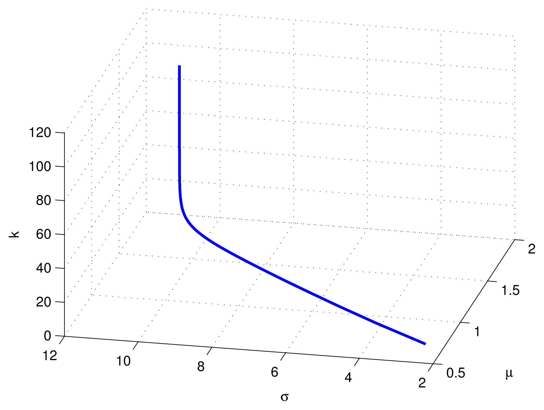
To start the simulation, the initial value is chosen as u0 = (μ0, σ0)T = (0.7, 2.5)T. The weights ɛ and λ are taken as 0.6 and 0.8, respectively. As a result, the response of the output PDFs is shown in Figure 3, in which y denotes the output of the system, p(y; μ, σ) denotes the PDF of the output y and k denotes the sample time.
In order to illustrate the effectiveness of the control law in detail, the comparison between the final controlled output PDF and the target function is shown in Figure 4, where the horizontal axis denotes the output y and the vertical axis denotes the PDF p(y; μ, σ) of y.
Obviously, the output PDF can be controlled to be a steady state shown in Figure 4. However, as we know, assume that A and B are two sets in a metric space (e.g., Euclidean space) with the distance function d; then, the distance d(A, B) = maxxA;yB d(x, y) may be larger than zero. Actually, in our simulation, the target PDF is in the set of second order polynomials, and the PDF p(y; μ, σ) of the output y is exponential. Therefore, the non-zero steady error still exists all of the time.
The response of the optimal control input sequences is shown in Figure 5, in which (μ, σ) denotes the input vector and k denotes the sample time.
From above, it can be concluded that the simulation results demonstrate the effectiveness of the presented method, which gives a solution to control the shape of the output PDF.

6. Conclusions

In this paper, we investigate the open-loop stochastic distribution control systems of multi-input and single output with a stochastic noise, via the advantage of information geometric theory.
(1)
By the statistical characterizations of the stochastic distribution control systems, we formulate the controller design in the frame of information geometry. By virtue of the natural gradient algorithm, a steepest descent algorithm is proposed.
(2)
The convergence of the obtained algorithm is proven.
(3)
An example is discussed in detail to demonstrate our algorithm.

Acknowledgments

The authors would like to express their sincere thanks to the referees for their valuable suggestions. This subject are supported by the National Natural Science Foundations of China, Nos. 10871218, 10932002, 61179031, and the Doctoral Program of Higher Education of China through Grant, No. 20131103120027. The work of Linyu Peng was supported by the Math Department of the University of Surrey and the China Scholarship Council. The work of Linyu Peng is also supported by JST-CREST.

Author Contributions

In this paper, Zhenning Zhang is in charge of the control theory and information geometric theory, Huafei Sun is in charge of the geometric theory and paper writing, Linyu Peng is in charge of the geometric theory and the simulation, and Lin Jiu is in charge of the topological theory. The authors have read and approved the final published manuscript.

Conflicts of Interest

The authors declare no conflict of interest.

References

  1. Rao, C.R. Infromation and accuracy attainable in the estimation of statistical parameters. Bull. Calcutta. Math. Soc 1945, 37, 81–91. [Google Scholar]
  2. Efron, B. Defining the curvature of a statistical problem. Ann. Stat 1975, 3, 1189–1242. [Google Scholar]
  3. Efron, B. The geometry of exponential families. Ann. Stat 1978, 6, 362–376. [Google Scholar]
  4. Chentsov, N.N. Statistical Decision Rules and Optimal Inference; AMS: Providence, RI, USA, 1982. [Google Scholar]
  5. Amari, S.; Nagaoka, H. Methods of Information Geometry; Oxford University Press: Oxford, UK, 2000. [Google Scholar]
  6. Amari, S. Differential Geometrical Methods in Statistics; Springer-Verlag: Berlin/Heidelberg, Germany,, 1990. [Google Scholar]
  7. Amari, S. Information geometry of the EM and em algorithm for neural networks. Neural Netw 1995, 8, 1379–1408. [Google Scholar]
  8. Amari, S.; Kurata, K.; Nagaoka, H. Information geometry of Boltzmann machines. IEEE Trans. Neural Netw 1992, 3, 260–271. [Google Scholar]
  9. Amari, S. Differential geometry of a parametric family of invertible linear systems-Riemannian metric, dual affine connections, and divergence. Math. Syst. Theory 1987, 20, 53–83. [Google Scholar]
  10. Zhang, Z.; Sun, H.; Zhong, F. Natural gradient-projection algorithm for distribution control. Optim. Control Appl. Methods 2009, 30, 495–504. [Google Scholar]
  11. Zhong, F.; Sun, H.; Zhang, Z. An Information geometry algorithm for distribution control. Bull. Braz. Math. Soc 2008, 39, 1–10. [Google Scholar]
  12. Zhang, Z.; Sun, H.; Peng, L. Natural gradient algorithm for stochastic distribution systems with output feedback. Differ. Geom. Appl 2013, 31, 682–690. [Google Scholar]
  13. Peng, L.; Sun, H.; Sun, D.; Yi, J. The geometric structures and instability of entropic dynamical models. Adv. Math 2011, 227, 459–471. [Google Scholar]
  14. Peng, L.; Sun, H.; Xu, G. Information geometric characterization of the complexity of fractional Brownian motions. J. Math. Phys 2012, 53, 123305. [Google Scholar]
  15. Amari, S. Natural gradient works efficiently in learning. Neural Comput 1998, 10, 251–276. [Google Scholar]
  16. Amari, S. Natural gradient learning for over- and under-complete bases in ICA. Neural Comput 1999, 11, 1875–1883. [Google Scholar]
  17. Park, H.; Amari, S.; Fukumizu, K. Adaptive natural gradient learning algorithms for various stochastic model. Neural Netw 2000, 13, 755–764. [Google Scholar]
  18. Guo, L.; Wang, H. Stochastic Distribution Control System Design: A Convex Optimization Approach; Springer: London, UK, 2010. [Google Scholar]
  19. Wang, H. Control of Conditional output probability density functions for general nonlinear and non-Gaussian dynamic stochastic systems. IEE Proc. Control Theory Appl 2003, 150, 55–60. [Google Scholar]
  20. Guo, L.; Wang, H. Minimum entropy filtering for multivariate stochastic systems with non-Gaussian noises. IEEE Trans. Autom. Control 2006, 51, 695–670. [Google Scholar]
  21. Wang, A.; Afshar, P.; Wang, H. Complex stochastic systems modelling and control via iterative machine learning. Neurocomputing 2008, 71, 2685–2692. [Google Scholar]
  22. Dodson, C.T.J.; Wang, H. Iterative approximation of statistical distributions and relation to information geometry. Stat. Inference Stoch. Process 2001, 4, 307–318. [Google Scholar]
  23. Wang, A.; Wang, H.; Guo, L. Recent Advances on Stochastic Distribution Control: Probability Density Function Control. Proceedings of the CCDC 2009: Chinese Control and Decision Conference, Guilin, China, 17–19 June 2009. [CrossRef]
  24. Sun, H.; Peng, L.; Zhang, Z. Information geometry and its applications. Adv. Math. (China) 2011, 40, 257–269. (In Chinese) [Google Scholar]
Figure 1. The stochastic distribution control systems.
Entropy 16 04338f1
Figure 2. The open-loop stochastic distribution control systems.
Entropy 16 04338f2
Figure 3. The response of the output probability density functions.
Entropy 16 04338f3
Figure 4. The final and the target probability density functions.
Entropy 16 04338f4
Figure 5. The optimal control input sequences.
Entropy 16 04338f5