Combinatorial Optimization with Information Geometry: The Newton Method

1. Introduction

In this paper, statistical exponential families [1] are thought of as differentiable manifolds along the approach called information geometry [2] or the exponential statistical manifold [3]. Specifically, our aim is to discuss optimization on statistical manifolds using the Newton method, as is suggested in ([4] (Ch. 5 and 6)); see also the monograph [5]. This method is based on classical Riemannian geometry [6], but here, we put our emphasis on coordinate-free differential geometry; see [7,8].

We mainly refer to the above-mentioned references [2,4], with one notable exception in the description of the tangent space. Our manifold will be an exponential family $ℰ$_V of positive densities, V being a vector space of sufficient statistics. Given a one-dimensional statistical model p(t) ∈ $ℰ$_V, t ∈ I, we define its velocity at time t to be its Fisher score $s(t)=\frac{d}{dt}\hspace{0.17em}\text{ln}\hspace{0.17em}p(t)$[9]. The Fisher score s(t) is a random variable with zero expectation with respect to p(t), [s(t)] = 0. Because of that, the tangent space at p ∈ $ℰ$_V is a vector space of random variables with zero expectation at p. A vector field is a mapping from p to a random variable V (p), such that for all p ∈ $ℰ$, the random variable V(p) is centered at p, [V(p)] = 0. In other words, each point of the manifold has a different tangent space, and this tangent space can be used as a non-parametric model space of the manifold. In this formalism, a vector field is a mapping from densities to centered random variables, that is, it is what in statistics is called a pivot of the statistical model. To avoid confusion with the product of random variables, we do not use the standard notation for the action of a vector field on a real function. This approach is possibly unusual in differential geometry, but it is fully natural from the statistical point of view, where the Fisher score has a central place. Moreover, this approach scales nicely from the finite state space to the general state space; see the discussion in [9] and the review in [3].

A complete construction of the geometric framework based on the idea of using the Fisher scores as elements of the tangent bundle has been actually worked out. In this paper, we go on by considering a second order geometry based on the non-parametric settings.

Our main motivation for such a geometrical construction is its application to combinatorial optimization using exponential families, whose first order version was developed in [10–14]. We give here an illustration of the methods in the following toy example.

Consider the function f(x₁, x₂) = a₀ + a₁x₁ + a₂x₂ + a₁₂x₁x₂, with x₁, x₂ = ±1, a₀, a₁, a₂, a₁₂ ∈ ℝ. The function f is a real random variable on the sample space Ω = {+1, −1}² with the uniform probability λ. Note that the coordinate mappings X₁,X₂ of Ω generate an orthonormal basis 1,X₁,X₂,X₁X₂ of L²(Ω, λ) and that f is the general form of a real random variable on such a space. Let ℘_> be the open simplex of positive densities on (Ω, λ), and let $ℰ$_V be a statistical model, i.e., a subset of ℘_>. The relaxed mapping F: $ℰ$_V → ℝ,

$$F(p)={\mathbb{E}}_p\hspace{0.17em}[f]=a_o+a_1{\mathbb{E}}_p\hspace{0.17em}[X_1]+a_2{\mathbb{E}}_p\hspace{0.17em}[X_2]=a_{12}{\mathbb{E}}_p\hspace{0.17em}[X_1{X}_2],$$

(1)

is strictly bounded by the maximum of f, F(p) = [f] < max_x∈Ω f(x), unless f is constant. We are looking for a sequence p_n, n ∈ ℕ, such that [f] → max_x∈Ω f(x) as n → ∞. The existence of such a sequence is a nontrivial condition for the model $ℰ$. Precisely, the closure of $ℰ$_V must contain a density, whose support is contained in the set of maxima {x ∈ Ω|f(x) = max f}. This condition is satisfied by the independence model, V = Span {X₁,X₂}, where we can write:

$$F({\eta }^1,{\eta }^2)=a_0+a_1{\eta }^1+a_2{\eta }^2+a_{12}{\eta }^1{\eta }^2,\mathrm{\hspace{0.17em} }\mathrm{\hspace{0.17em} }\mathrm{\hspace{0.17em} }{\eta }^i={\mathbb{E}}_p\hspace{0.17em}[X_i],$$

(2)

See Figure 1.

The gradient of Equation (2) has components ∂₁F = a₁ + a₁₂η², ∂₂F = a₂ + a₁₂η¹, and the flow along the gradient produces increasing values for F; however, the gradient flow does not converge to the maximum of F; see the dotted line in Figure 2. However, one can follow the suggestion by [15] and use a modified gradient (the “natural” gradient) flow that produces better results in our problem; see Figure 3. Full details on this example are given in Section 2.5.2.

In combinatorial optimization, the values of the function f are assumed to be available at each point, and the curve of steepest ascent of the relaxed function is learned through a simulation procedure based on exponential statistical models.

In this paper, we introduce, in Section 2, the geometry of exponential families and its first order calculus. The second order calculus and the Hessian are discussed in Section 3. Finally, in Section 4, we apply the formalism to the discussion of the Newton method in the context of the maximization of the relaxed function.

2. Models on a Finite State Space

We consider here the exponential statistical manifold on the set of positive densities on a measure space (Ω, μ) with Ω finite and counting measure μ. The setup we describe below is not strictly required in the finite case, because in such a case, other approaches are possible, but it provides a mathematical formalism that has its own pros and that scales naturally to the infinite case.

We provide below a schematic presentation of our formalism as an introduction to this section.

• Two different exponential families can actually be the same statistical model, as the set of densities in the two exponential families are actually equal. This fact is due to both the arbitrariness of the reference density and the fact that sufficient statistics are actually a vector basis of the vector space generated by the sufficient statistics. In a non-parametric approach, we can refer directly to the vector space of centered log-densities, while the change of reference density is geometrically interpreted as a change of chart. The set of all possible such charts defines a manifold.
• We make a specific interpretation of the tangent bundle as the vector space of Fisher’s scores at each density and use such tangent spaces as the space of coordinates. This produces a different tangent space/space of coordinates at each density, and different tangent spaces are mapped one onto another by a proper parallel transport, which is nothing else than the re-centering of random variables.
• If a basis is chosen, a parametrization is given, and such a parametrization is, in fact, a new chart, whose values are real vectors. In the real parametrization, the natural scalar product in each scores space is given by Fisher’s information matrix.
• Riemannian gradients are defined in the usual way. It is customary in information geometry to call “natural gradient” the real coordinate presentation of the Riemannian gradient. The natural gradient is computed by applying the inverse of the Fisher information matrix to the Euclidean gradient. It seems that there are tree gradients involved, but they all represent the same object when correctly understood.
• The classical notion of expectation parameters for exponential families carries on as another chart on the statistical manifold, which gives rise to a further presentation of a geometrical object.
• While the statistical manifold is unique, there are at least three relevant connections as structures on the vector bundles of the manifold: one relating to the exponential charts, one relating to the expectation charts and one depending on the Riemannian structure.

2.1. Exponential Families As Manifolds

On the finite sample space Ω, #Ω = n, let a set of random variables $ℬ$ = {X₁, . . . ,X_m} be given, such that ∑_Jα_jX_j is constant if, and only if, the α_j’s are zero, or, equivalently, such that X₀ = 1,X₁, . . . ,X_m are affinely independent. The condition implies, necessarily, the linear independence of $ℬ$. A common choice is to take a set of linearly independent and μ-centered random variables.

We write = Span {X₁, . . . ,X_m} and define the following exponential family of positive densities p ∈ ℘_>:

$${\mathcal{E}}_V=\{q\in {\mathcal{P}}_{>}\mid q\propto {\text{e}}^{V}p,V\in \mathcal{V}\}.$$

(3)

Given any couple p, q ∈ , then there exist a unique set of parameters θ = θ_p(q), such that:

$$q=\text{exp}\hspace{0.17em}\left(\sum _j{\theta }^j\hspace{0.17em}{{}^e\mathbb{U}}^p{X}_j-{\psi }_p(\mathit{\theta })\right)·p$$

(4)

where is the centering at p, that is,

$${{}^e\mathbb{U}}^p:\mathcal{V}\notin U\mapsto U-{\mathbb{E}}_p\hspace{0.17em}[U]\in {{}^e\mathbb{U}}^p\mathcal{V}.$$

(5)

The linear mapping is one-to-one on and X_j, j = 1, . . . ,m, and is a basis of . We view each choice of a specific reference p as providing a chart centered at p on the exponential family , namely:

$${\sigma }_p:\text{exp}\hspace{0.17em}\left(\sum _j{\theta }^j\hspace{0.17em}{{}^e\mathbb{U}}^p{X}_j-{\psi }_p(\mathit{\theta })\right)·p\mapsto \mathit{\theta },$$

(6)

If:

$$U={{}^e\mathbb{U}}^{p}U+{\mathbb{E}}_p\hspace{0.17em}[U]=\sum _{j=1}^m{\theta }^j\hspace{0.17em}{{}^e\mathbb{U}}^p{X}_j+{\mathbb{E}}_p\hspace{0.17em}[U],$$

(7)

then:

$${\mathbb{E}}_p\hspace{0.17em}[U\hspace{0.17em}{{}^e\mathbb{U}}^p{X}_i]=\sum _{j=1}^m{\theta }^j\hspace{0.17em}{\mathbb{E}}_p\hspace{0.17em}[{{}^e\mathbb{U}}^p\hspace{0.17em}{X}_i\hspace{0.17em}{{}^e\mathbb{U}}^p{X}_j],$$

(8)

so that $\mathit{\theta }=I_{\mathcal{B}}^{-1}(p){\mathbb{E}}_p\hspace{0.17em}[U\hspace{0.17em}{{}^e\mathbb{U}}^p\mathit{X}]$, where:

$$I_{\mathcal{B}}(p)={[{\text{Cov}}_p(X_i,X_j)]}_{ij}={\mathbb{E}}_p\hspace{0.17em}[\mathit{X}\hspace{0.17em}{\mathit{X}}^{\prime }]-{\mathbb{E}}_p\hspace{0.17em}[\mathit{X}]\hspace{0.17em}{\mathbb{E}}_p\hspace{0.17em}[{\mathit{X}}^{\prime }]$$

(9)

is the Fisher information matrix of the basis $ℬ$ = {X₁, . . . ,X_m}.

The mappings:

$${\sigma }_p:{\mathcal{E}}_{\mathcal{V}}\ni q\mapsto U\mapsto \mathit{\theta }\in {\mathbb{R}}^m$$

(10)

where:

$$s_p:q\mapsto U=\text{log}\hspace{0.17em}\left(\frac{q}{p}\right)-{\mathbb{E}}_p\hspace{0.17em}\left[\text{log}\hspace{0.17em}\left(\frac{q}{p}\right)\right],$$

(11)

$${\sigma }_p:q\mapsto \mathit{\theta }=I_{\mathcal{B}}^{-1}(p)\hspace{0.17em}{\mathbb{E}}_p\hspace{0.17em}[U\hspace{0.17em}{{}^e\mathbb{U}}^p\mathit{X}]=I_{\mathcal{B}}^{-1}(p)\hspace{0.17em}{\mathbb{E}}_p\hspace{0.17em}\left[\text{log}\hspace{0.17em}\left(\frac{q}{p}\right)\hspace{0.17em}{{}^e\mathbb{U}}^p\mathit{X}\right],$$

(12)

are global charts in the non-parametric and parametric coordinates, respectively. Notice that Equation (12) provides the regression coefficients of the least squares estimate on of the log-likelihood.

We denote by e_p : ℝ^m → the inverse of σ_p, i.e.,

$$e_p(\mathit{\theta })=\text{exp}\hspace{0.17em}\left(\sum _{j=1}^m{\theta }^j\hspace{0.17em}{{}^e\mathbb{U}}^p{X}_j-{\psi }_p(\mathit{\theta })\right)·p,$$

(13)

so that the representation of the divergence q ↦ D(p ||q) in the chart σ_p is ψ_p:

$${\psi }_p(\mathit{\theta })=\text{log}\hspace{0.17em}\left({\mathbb{E}}_p\hspace{0.17em}\left[e^{{\sum }_{j=1}^m{\theta }^j\hspace{0.17em}{{}^e\mathbb{U}}^p{X}_j}\right]\right)={\mathbb{E}}_0\hspace{0.17em}\left[\text{log}\hspace{0.17em}\left(\frac{p}{e_p(\mathit{\theta })}\right)\right]=\text{D}\hspace{0.17em}(p\Vert e_p(\mathit{\theta })).$$

(14)

The mapping I_$ℬ$: p ↦ Cov_p (X, X) ∈ ℝ^m×m is represented in the chart centered at p by:

$$I_{\mathcal{B},p}(\mathit{\theta })=I_{\mathcal{B}}(e_p(\mathit{\theta }))={[{\text{Cov}}_{e_p(\mathit{\theta })}\hspace{0.17em}(X_i,X_j)]}_{i,j}=\text{Hess\hspace{0.17em}}{\psi }_p(\mathit{\theta }),$$

(15)

See [1].

2.2. Change of Chart

Fix p, p̄ ∈ ; then, we can express p in the chart centered at p̄,

$$p=\text{exp}\hspace{0.17em}\left(\overline{U}-k_p(\overline{U})\right)·\overline{p},\mathrm{\hspace{0.17em} }\mathrm{\hspace{0.17em} }\mathrm{\hspace{0.17em} }\overline{U}\in {{}^e\mathbb{U}}^{\overline{p}}\mathcal{V},\mathrm{\hspace{0.17em} }\mathrm{\hspace{0.17em} }\mathrm{\hspace{0.17em} }{k}_{\overline{p}}(\overline{U})=\text{log}\hspace{0.17em}\left({\mathbb{E}}_{\overline{p}}\hspace{0.17em}\left[{\text{e}}^{\overline{U}}\right]\right).$$

(16)

In coordinates $\overline{U}={\sum }_{j=1‘}^m{\overline{\theta }}^j\hspace{0.17em}{{}^e\mathbb{U}}^{\overline{p}}{X}_j$.

For all q ∈ , q = exp (U − k_p(U)) p, U ∈ , k_p(U) = log ( [e^U]), in coordinates $U={\sum }_{j=1‘}^m{\theta }^j\hspace{0.17em}{{}^e\mathbb{U}}^p{X}_j$, we can write:

$$\begin{array}{l}q=\text{exp\hspace{0.17em}}(U-k_p(U))·p\\ =\text{exp\hspace{0.17em}}(U-k_p(U))\hspace{0.17em}\text{exp\hspace{0.17em}}(\overline{U}-k_{\overline{p}}(\overline{U}))·\overline{p}\\ =\text{exp\hspace{0.17em}}(U-k_p(U)+\overline{U}-k_{\overline{p}}(\overline{U}))·\overline{p}\\ =\text{exp\hspace{0.17em}}(((U+\overline{U})-{\mathbb{E}}_{\overline{p}}[U])-\hspace{0.17em}(k_p(U)-k_{\overline{p}}(\overline{U})+{\mathbb{E}}_{\overline{p}}[U]))·\overline{p},\end{array}$$

(17)

hence, the non-parametric coordinate of q in the chart centered at p̄ is U + Ū − [U] = (U) + Ū.

From Equation (12):

$$\begin{array}{l}{\sigma }_{\overline{p}}(q)=I_{\mathcal{V}}^{-1}(\overline{p}){\mathbb{E}}_{\overline{p}}\hspace{0.17em}[({{}^e\mathbb{U}}^{\overline{p}}U+\overline{U}){{}^e\mathbb{U}}^{\overline{p}}\mathit{X}]\\ =\mathit{\theta }+\overline{\mathit{\theta }}\end{array}$$

(18)

This provides the change of charts ${\sigma }_{\overline{p}}\circ {\sigma }_p^{-1}:\mathit{\theta }\mapsto \mathit{\theta }+\overline{\mathit{\theta }}$. This atlas of charts defines the affine manifold ( , (σ_p)). This fact has deep consequences that we do not discuss here, e.g., our manifold is an instance of a Hessian manifold [16].

2.3. Tangent Bundle

The space of Fisher scores at p is , and it is identified with the tangent space of the manifold at p, T_q ; see the discussion in [3,9]. Let us check the consistency of this statement with our θ-parametrization.

Let:

$$q(\tau )=\text{exp}\hspace{0.17em}\left(\sum _{j=1}^m{\theta }^j(\tau ){{}^e\mathbb{U}}^{q(0)}\mathit{X}-{\psi }_{q(0)}(\tau )\right)·q(0),$$

(19)

τ ∈ I, I an open interval containing zero, a curve in . In the chart centered at q(0), we have from Equation (12):

$$\begin{array}{l}{\sigma }_{q(0)}(q(\tau ))=I_{\mathcal{B}}^{-1}(q(0))\hspace{0.17em}{\mathbb{E}}_{q(0)}\hspace{0.17em}\left[\text{log}\hspace{0.17em}\left(\frac{q(\tau )}{q(0)}\right)\hspace{0.17em}{{}^e\mathbb{U}}^{q(0)}\mathit{X}\right]\\ =I_{\mathcal{B}}^{-1}(q(0))\hspace{0.17em}{\mathbb{E}}_{q(0)}\hspace{0.17em}\left[\left(\sum _{j=1}^m{\theta }^j(\tau )\hspace{0.17em}{{}^e\mathbb{U}}^{q(0)}{X}_j-{\psi }_{q(0)}(\mathit{\theta }(\tau ))\right)\hspace{0.17em}{{}^e\mathbb{U}}^{q(0)}\mathit{X}\right]\\ =I_{\mathcal{B}}^{-1}(q(0))\sum _{j=1}^m{\theta }^j(\tau ){\mathbb{E}}_{q(0)}\hspace{0.17em}\left[{{}^e\mathbb{U}}^{q(0)}{X}_j{{}^e\mathbb{U}}^{q(0)}\mathit{X}\right]\\ =I_{\mathcal{B}}^{-1}(q(0))\hspace{0.17em}{\mathbb{E}}_{q(0)}\hspace{0.17em}\left[{{}^e\mathbb{U}}^{q(0)}\mathit{X}\hspace{0.17em}{{}^e\mathbb{U}}^{q(0)}\mathit{X}\right]\hspace{0.17em}\mathit{\theta }\\ =\mathit{\theta }(\tau ).\end{array}$$

(20)

The vector space is represented by the coordinates in the base $ℬ$. The tangent bundle T as a manifold is defined by the charts (σ_p, σ̇_p) on the domain:

$$T{\mathcal{E}}_{\mathcal{V}}=\{(p,v)\mid p\in {\mathcal{E}}_{\mathcal{V}},v\in T_p{\mathcal{E}}_{\mathcal{V}}\}$$

(21)

with:

$$({\sigma }_p,{\dot{\sigma }}_p):(q,V)\mapsto \left(I_{\mathcal{B}}^{-1}(p)\hspace{0.17em}{\mathbb{E}}_p\hspace{0.17em}\left[\text{log}\hspace{0.17em}\left(\frac{q}{p}\right)\hspace{0.17em}{{}^e\mathbb{U}}^p\mathit{X}\right],I_{\mathcal{B}}^{-1}(p)\hspace{0.17em}{\mathbb{E}}_p\hspace{0.17em}[V\hspace{0.17em}{{}^e\mathbb{U}}^p\mathit{X}]\right).$$

(22)

The dot notation σ̇_p for the charts on the tangent spaces is justified by the computation in Equation (23) below:

$${\frac{d}{dt}{\sigma }_{q(0)}(q(\tau ))|}_{\tau =0}=I_{\mathcal{B}}^{-1}(q(0))\hspace{0.17em}{\mathbb{E}}_{q(0)}\hspace{0.17em}\left[{\frac{d}{dt}\text{log}(q(\tau ))|}_{\tau =0}{{}^e\mathbb{U}}^{q(0)}\mathit{X}\right]=I_{\mathcal{B}}^{-1}(q(0))\hspace{0.17em}{\mathbb{E}}_{q(0)}\hspace{0.17em}\left[\delta q(0)\hspace{0.17em}{{}^e\mathbb{U}}^{q(0)}\mathit{X}\right]={\dot{\sigma }}_{q(0)}(\delta q(0)).$$

(23)

The velocity at τ = 0 is $\delta q(0)={\frac{d}{d\tau }\text{log\hspace{0.17em}}(q(\tau ))\mid }_{\tau =0}\in T_{q(0)}{\mathcal{E}}_{\mathcal{V}}$ and:

$$\begin{array}{l}{\frac{d}{d\tau }\mathit{\theta }(\tau )|}_{\tau =0}=I_{\mathcal{B}}^{-1}(q(0))\hspace{0.17em}{\mathbb{E}}_{q(0)}\hspace{0.17em}\left[{\frac{d}{d\tau }\text{log}(q(\tau ))|}_{\tau =0}{{}^e\mathbb{U}}^{q(0)}\mathit{X}\right]\\ =I_{\mathcal{B}}^{-1}(q(0))\hspace{0.17em}{\mathbb{E}}_{q(0)}\hspace{0.17em}\left[\delta q(0)\hspace{0.17em}{{}^e\mathbb{U}}^{q(0)}\mathit{X}\right],\end{array}$$

(24)

which is consistent with both the definition of tangent space as set of Fisher scores and with the chart of the tangent bundle as defined in Equation (22).

The velocity at a generic τ is $\delta q(\tau )=\frac{d}{d\tau }\text{log\hspace{0.17em}}(q(\tau ))\in T_{q(\tau )}{\mathcal{E}}_{\mathcal{V}}$ and has coordinates at p:

$$\begin{array}{l}\frac{d}{d\tau }\mathit{\theta }(\tau )=I_{\mathcal{B}}^{-1}(q(0))\hspace{0.17em}{\mathbb{E}}_{q(0)}\hspace{0.17em}\left[\frac{d}{d\tau }\text{log}(q(\tau ))\hspace{0.17em}{{}^e\mathbb{U}}^{q(0)}\mathit{X}\right]\\ =I_{\mathcal{B}}^{-1}(q(0))\hspace{0.17em}{\mathbb{E}}_{q(0)}\hspace{0.17em}\left[\delta q(\tau )\hspace{0.17em}{{}^e\mathbb{U}}^{q(0)}\mathit{X}\right].\end{array}$$

(25)

If V,W are vector fields on T , i.e., V (p),W(p) ∈ T_p = , p ∈ , we define a Riemannian metric g(V,W)) by:

$$g(V,W)(p)=g_p(V(p),W(p))={\mathbb{E}}_p\hspace{0.17em}[V(p)W(p)]$$

(26)

In coordinates at p, $V(p)={\sum }_j{\dot{\sigma }}_p^j(V)\hspace{0.17em}{{}^e\mathbb{U}}^p{X}_j,W(p)={\sum }_j{\dot{\sigma }}_p^j(W)\hspace{0.17em}{{}^e\mathbb{U}}^p{X}_j$, so that:

$$g_p(V(p),W(p))={\dot{\sigma }}_p{(V)}^{\prime }{I}_{\mathcal{B}}(p){\dot{\sigma }}_p(W).$$

(27)

2.4. Gradients

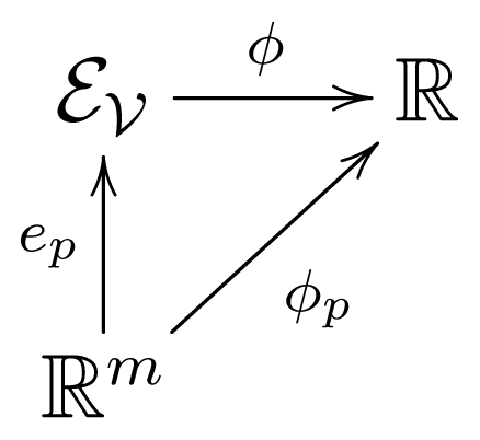
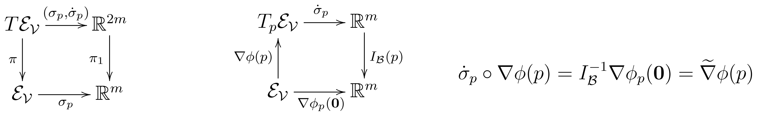
Given a function φ: → ℝ let φ_p = φ ∘ e_p, $e_p={\sigma }_p^{-1}$, its representation in the chart centered at p:

(28)

The derivative of θ ↦ φ_p(θ) at θ = 0 along α ∈ ℝ^m is:

$$\nabla {\phi }_p(\mathbf{0})\mathit{\alpha }=\nabla {\phi }_p(\mathbf{0})I_{\mathcal{B}}^{-1}(p)I_{\mathcal{B}}(p)\mathit{\alpha }={(I_{\mathcal{B}}^{-1}(p)\nabla {\phi }_p{(\mathbf{0})}^{\prime })}^{\prime }{I}_{\mathcal{B}}(p)\mathit{\alpha }=g_p(I_{\mathcal{B}}^{-1}(p)\nabla {\phi }_p{(\mathbf{0})}^{\prime },\mathit{\alpha }).$$

(29)

The mapping $\tilde{\nabla }\phi :p\mapsto I_{\mathcal{B}}^{-1}(p){(\nabla {\phi }_p(\mathbf{0}))}^{\prime }\in {\mathbb{R}}^m$ that appears in Equation (29) is Amari’s natural gradient of φ: ; see [15]. It is a standard notion in Riemannian geometry; cf. [4] (p. 46).

More generally, the derivative of θ ↦ φ_p(θ) at θ along α ∈ ℝ^m is:

$$\nabla {\phi }_p(\mathit{\theta })\mathit{\alpha }=\nabla {\phi }_p(\mathit{\theta })I_{\mathcal{B}}^{-1}(e_p(\mathit{\theta }))I_{\mathcal{B}}(e_p(\mathit{\theta }))\mathit{\alpha }={(I_{\mathcal{B}}^{-1}(e_p(\mathit{\theta }))\nabla {\phi }_p{(\mathit{\theta })}^{\prime })}^{\prime }{I}_{\mathcal{B}}(e_p(\mathit{\theta }))\mathit{\alpha }=g_{e_p(\mathit{\theta })}(I_{\mathcal{B}}^{-1}(e_p(\mathit{\theta }))\nabla {\phi }_p{(\mathit{\theta })}^{\prime },\mathit{\alpha }).$$

(30)

Let us compare ∇φ_q(0) and ∇φ_p(θ) when q = e_p(θ). As φ_p = φ ∘ e_p and φ_q = φ ∘ e_q, we have the change of charts:

$${\phi }_q=\phi \circ e_q=\phi \circ e_p\circ {\sigma }_p\circ e_q={\phi }_p\circ {\sigma }_p\circ e_q,$$

(31)

hence ∇φ_q(0) = ∇φ_p(σ_p(q))J(σ_p ∘ e_q)(0), where J(σ_p ∘ e_q) is the Jacobian of σ_p ∘ e_q. As σ_p ∘ e_q(θ) = θ + σ_p(q), we have J(σ_p ∘ e_q) = Id, and in conclusion, ∇φ_ep(θ)(0) = ∇φ_p(θ). For all p ∈ and θ ∈ ℝ^m,

$$\tilde{\nabla }\phi (e_p(\theta ))=I_{\mathcal{B}}^{-1}(e_p(\theta ))\nabla {\phi }_p(\theta ).$$

(32)

Alternatively, for all q, p ∈ , ∇̃φ: → ℝ^m is defined by:

$$\tilde{\nabla }\phi (q)=I_{\mathcal{B}}^{-1}(q)\nabla {\phi }_p({\sigma }_p(q)).$$

(33)

The Riemannian gradient of φ: is the vector field ∇φ, such that D_Yφ = g(∇φ, Y ). Note that the Riemannian gradient takes values in the tangent bundle, while the natural gradient takes values in ℝ^m. We compute the Riemannian gradient at p as follows. If y = σ̇_p(Y (p)),

$$D_Y\phi (p)=d{\phi }_p(\mathbf{0})\mathit{y}=g_p(\tilde{\nabla }\phi (p),\mathit{y})={\mathbb{E}}_p\hspace{0.17em}[\nabla \phi (p)Y(p)],$$

(34)

hence $\tilde{\nabla }\phi (p)=I_{\mathcal{B}}^{-1}(p)\nabla {\phi }_p{(\mathbf{0})}^{\prime }$ is the representation in the chart centered at p of the vector field ∇φ: . Explicitly, we have (see Equation (22)),

$$\tilde{\nabla }\phi (p)=I_{\mathcal{B}}^{-1}(p){(\nabla {\phi }_p(\mathbf{0}))}^{\prime }=I_{\mathcal{B}}^{-1}(p)\hspace{0.17em}{\mathbb{E}}_p\hspace{0.17em}[\nabla \phi (p)\hspace{0.17em}{{}^e\mathbb{U}}^p\mathit{X}],$$

(35)

$$\nabla \phi (p)=\sum _j{(\tilde{\nabla }\phi (p))}^j\hspace{0.17em}{{}^e\mathbb{U}}^p{X}_j$$

(36)

The Euclidean gradient ∇φ_p(θ) is sometimes called the “vanilla gradient.” It is equal to the covariance between the Riemannian gradient ∇φ(p) and the basis X, (∇φ_p(0))′ = [∇φ(p) X].

We summarize in a display the relations between our three gradients: Euclidean ∇φ_p(0), natural ∇̃φ(p) and Riemannian ∇φ(p).

(37)

In the following, we shall frequently use the fact that the representation of the gradient vector field ∇φ in a generic chart centered at p is:

$${(\nabla \phi )}_p(\mathit{\theta })={\dot{\sigma }}_p(\nabla \phi (e_p(\mathit{\theta })))=(\tilde{\nabla }\phi )(e_p(\mathit{\theta }))=I_{\mathcal{B},p}^{-1}(\mathit{\theta })\nabla {\phi }_p(\mathit{\theta }).$$

(38)

It should be noted that the leftmost term (∇φ)_p(θ) is the presentation of the gradient in the charts of the tangent bundle, while in the rightmost term, ∇φ_p(θ) denotes the Euclidean gradient of the presentation of the function φ in the charts of the manifold.

2.4.1. Expectation Parameters

As ψ_p is strictly convex, the gradient mapping θ ↦ (∇ψ_p(θ))′ is a homeomorphism from the space of parameters ℝ^m to the interior of the convex set generated by the image of X; see [1]. The function μ_p : defined by:

$${\mu }_p(q)={\mathbb{E}}_q\hspace{0.17em}[{{}^e\mathbb{U}}^p\mathit{X}]={\mathbb{E}}_q\hspace{0.17em}[\mathit{X}]-{\mathbb{E}}_p\hspace{0.17em}[\mathit{X}]={(\nabla {\psi }_p(\mathit{\theta }))}^{\prime },\mathrm{\hspace{0.17em} }\mathrm{\hspace{0.17em} }\mathrm{\hspace{0.17em} }\mathit{\theta }={\sigma }_p(q)$$

(39)

is a chart for all p ∈ . The value of the inverse q = L_p(μ) is characterized as the unique q ∈ , such that μ = [ X], i.e., the maximum likelihood estimator.

Let us compute the change of chart from p to p̄:

$${\mu }_{\overline{p}}\circ {\mu }_p^{-1}(\mathit{\eta })=\overline{\mathit{\eta }}=\mathit{\eta }+{\mathbb{E}}_p\hspace{0.17em}[\mathit{X}]-{\mathbb{E}}_{\overline{p}}\hspace{0.17em}[\mathit{X}].$$

(40)

In fact, μ = [ X] and μ̄ = μ_p̄(L_p(μ)) = [ X].

We do not discuss here the rich theory started in [2] about the duality between σ_p and μ_p. We limit ourselves to the computation of the Riemannian gradient in the expectation parameters. If φ: ,

$${\phi }_p(\mathit{\theta })=\phi \circ e_p(\mathit{\theta })=\phi \circ L_p\circ {\mu }_p\circ e_p(\mathit{\theta })=(\phi \circ L_p)\circ (\nabla {\psi }_p)(\mathit{\theta }),$$

(41)

because μ_p ∘ e_p(θ) = [ X] = ∇φ_p(θ), hence:

$$\nabla {\phi }_p(\mathit{\theta })=\nabla (\phi \circ L_p)(\nabla {\psi }_p(\mathit{\theta }))\hspace{0.17em}\text{Hess\hspace{0.17em}}{\psi }_p(\mathit{\theta }),$$

(42)

$$\tilde{\nabla }\phi (p)=I_{\mathcal{V}}{(p)}^{-1}{(\nabla (\phi \circ L_p)(\mathbf{0})\hspace{0.17em}\text{Hess\hspace{0.17em}}{\psi }_p(\mathit{\theta }))}^{\prime }={(\nabla (\phi \circ L_p)(\mathbf{0}))}^{\prime },$$

(43)

$$\nabla \phi (p)=\nabla (\phi \circ L_p)(\mathbf{0})\hspace{0.17em}{{}^e\mathbb{U}}^p\mathit{X},$$

(44)

that is, the natural gradient ∇̃φ at p = L_p(μ) is equal to the Euclidean gradient of μ ↦ φ ∘ L_p(μ) at μ = 0.

2.4.2. Vector Fields

If V is a vector field of T and φ: is a real function, then we define the action of V on φ, ∇_V φ, to be the real function:

$${\nabla }_V\phi :{\mathcal{E}}_{\mathcal{V}}\ni p\mapsto {\nabla }_V\phi (p)=\nabla {\phi }_p(\mathbf{0}){\dot{\sigma }}_p(V(p)).$$

(45)

We prefer to avoid the standard notation V φ, because in our setting, V (p) is a random variable, and the product V (p)φ(p) is otherwise defined as the ordinary product.

Let us represent ∇_V φ in the chart centered at p:

$${({\nabla }_V\phi )}_p(\mathit{\theta })={\nabla }_V\phi (e_p(\mathit{\theta }))=\nabla {\phi }_{e_p(\mathit{\theta })}(\mathbf{0}){\dot{\sigma }}_{e_p(\mathit{\theta })}(V(e_p(\mathit{\theta })))=\nabla {\phi }_p(\mathit{\theta })V_p(\mathit{\theta }),$$

(46)

where we have used the equality ∇φ_{ep (θ)}(0) = ∇φ_p(θ) and V_p(θ) = σ̇_ep(θ) (V (e_p(θ))).

If W is a vector field, we can compute ∇_W∇_V φ at p as:

$$\begin{array}{l}{\nabla }_W{\nabla }_V\phi (p)=\nabla {({\nabla }_V\phi )}_p(\mathbf{0}){\dot{\sigma }}_p(W(p))\\ =V_p{(\mathbf{0})}^{\prime }\text{Hess\hspace{0.17em}}{\phi }_p(\mathbf{0})W_p(\mathbf{0})+\nabla {\phi }_p(\mathbf{0})J{V}_p(\mathbf{0})W_p(\mathbf{0}),\end{array}$$

(47)

where J denotes the Jacobian matrix.

The Lie bracket [W, V ]φ (see [7] (§4.2), [8] (V, §1), [4] (Section 5.3.1)) is given by:

$$[W,V]\phi (p)={\nabla }_W{\nabla }_V\phi (p)-{\nabla }_V{\nabla }_w\phi (p)=\nabla {\phi }_p(\mathbf{0})\hspace{0.17em}(J{V}_p(\mathbf{0})W_p(\mathbf{0})-J{W}_p(\mathbf{0})V_p(\mathbf{0})),$$

(48)

because of Equation (47) and the symmetry of the Hessian.

The flow of the smooth vector field V : is a family of curves γ(t, p), p ∈ t ∈ J_p, J_p open real interval containing zero, such that for all p ∈ and t ∈ J_p,

$$\gamma (0,p)=p,$$

(49)

$$\delta \gamma (t,p)=V(\gamma (t,p)).$$

(50)

As uniqueness holds in Equation (50) (see [8] (VI, §1) or [7] (§4.1)), we have semi-group property γ(s + t, p) = γ(s, γ (t, p)), and Equation (50) is equivalent to δγ(0, p) = V (γ(0, p)), p ∈ .

If a flow of V is available, we have an interpretation of ∇_Vφ as a derivative of φ along (t, p),

$${\frac{d}{dt}\phi (\gamma (t,p))|}_{t=0}={\nabla {\phi }_p({\sigma }_p(\gamma (t,p)))\hspace{0.17em}\left(\frac{d}{dt}{\sigma }_p(\gamma (t,p))\right)|}_{t=0}=\nabla {\phi }_p(\mathbf{0})V(p)={\nabla }_V\phi (p).$$

(51)

2.5. Examples

The following examples are intended to show how the formalism of gradients is usable in performing basic computations.

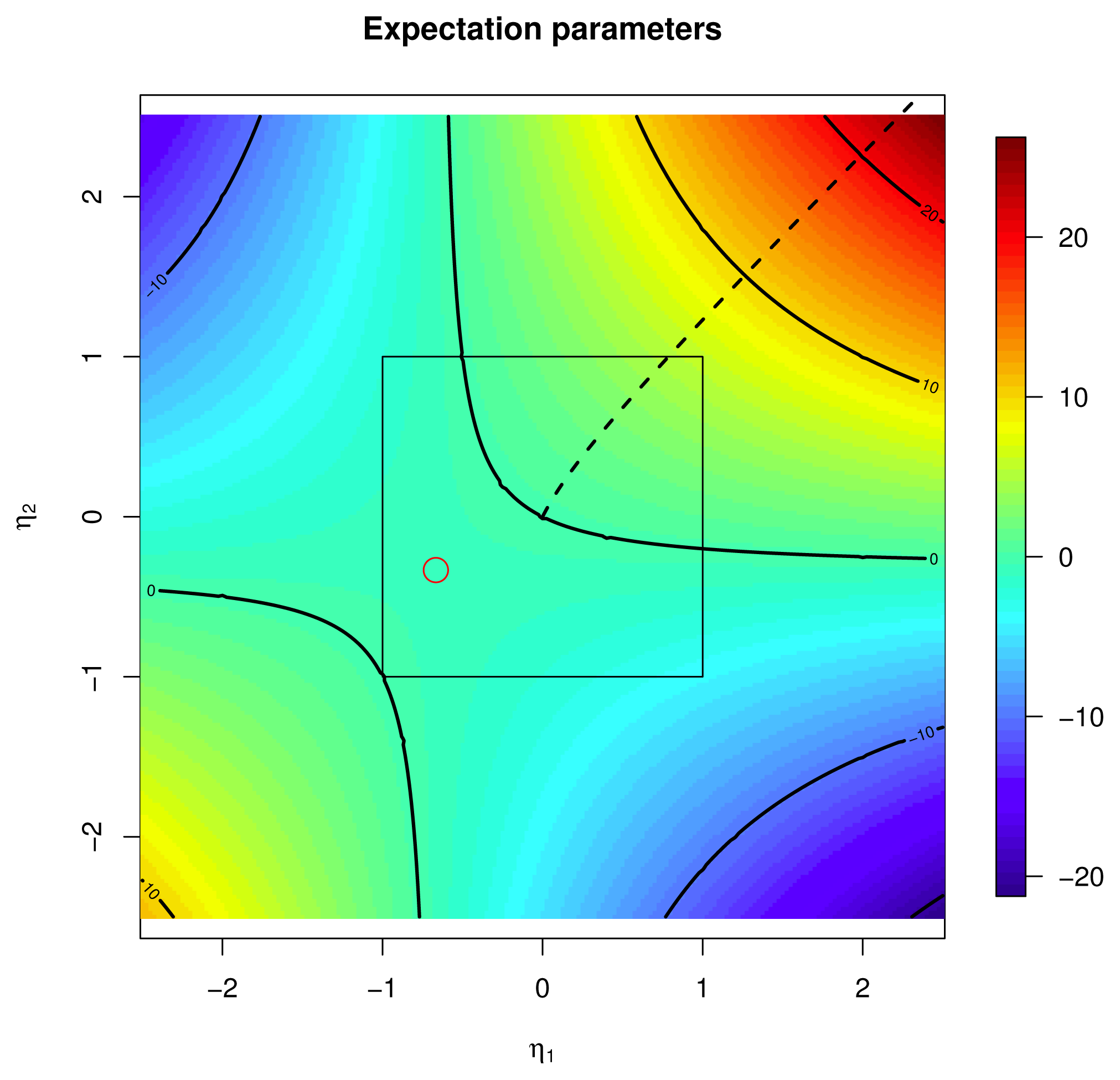
2.5.1. Expectation

Let f be any random variable, and define F : by F(p) = [f]. In the chart centered at p, we have:

$$F_p(\mathit{\theta })=\int f\text{exp}\hspace{0.17em}\left(\sum _j{\theta }^j\hspace{0.17em}{{}^e\mathbb{U}}^p{X}_j-{\psi }_p(\mathit{\theta })\right)·p\hspace{0.17em}d\mu$$

(52)

and the Euclidean gradient:

$$\nabla F_p(\mathbf{0})={\text{Cov}}_p(f,\mathit{X})\in {({\mathbb{R}}^m)}^{\prime }.$$

(53)

The natural gradient is:

$$\tilde{\nabla }F(p)={\text{Cov}}_p{(\mathit{X},\mathit{X})}^{-1}\hspace{0.17em}{\text{Cov}}_p(\mathit{X},f)\in {\mathbb{R}}^m,$$

(54)

and the Riemannian gradient is:

$$\nabla F(p)={(\tilde{\nabla }F(p))}^{\prime }{{}^e\mathbb{U}}^p\mathit{X}={\text{Cov}}_p(f,\mathit{X})\hspace{0.17em}{\text{Cov}}_p{(\mathit{X},\mathit{X})}^{-1}\hspace{0.17em}{{}^e\mathbb{U}}^p\mathit{X}\in T_p{\mathcal{E}}_{\mathcal{V}}.$$

(55)

From Equation (55), it follows that ∇F(p) is the L²(p)-projection f onto , while ∇̃F(p) in Equation (54) are the coordinates of the projection. Let us consider the family of curves:

$$\gamma (t,p)=\text{exp}\hspace{0.17em}\left(\sum _{j=1}^{m}t{(\tilde{\nabla }F(p))}^j\hspace{0.17em}{{}^e\mathbb{U}}^p{X}_j-{\psi }_p(t\tilde{\nabla }F(p))\right)·p,\mathrm{\hspace{0.17em} }\mathrm{\hspace{0.17em} }\mathrm{\hspace{0.17em} }t\in \mathbb{R}.$$

(56)

The velocity is:

$$\delta \gamma (t,p)=\frac{d}{dt}\hspace{0.17em}\left(\sum _{j=1}^{m}t{(\tilde{\nabla }F(p))}^j\hspace{0.17em}{{}^e\mathbb{U}}^p{X}_j-{\psi }_p(t\tilde{\nabla }F(p))\right)=\nabla F(p)-{\mathbb{E}}_{\gamma (t,p)}[\nabla F(p)],$$

(57)

which is different from ∇F(γ(t, p)), unless f ∈ ⊕ ℝ. Then, γ is not, in general, the flow of ∇F, but it is a local approximation, as δγ(0, p) = ∇F(p).

These computation are the basis of model-based methods in combinatorial optimization; see [10–14].

2.5.2. Binary Independent Variables

Here, we present, in full generality, the toy example of the Introduction; see [17] for more information on the application to combinatorial optimization. Our example is a very special case of Ising exactly solvable models [18], our aim being here to explore the geometric framework.

Let Ω = {+1, −1}^m with counting measure μ, and let the space be generated by the coordinate projections $ℬ$ = {X₁, . . . , X_d}. Note that we use here the coding +1, −1 (from physics) instead of the coding 0, 1, which is more common in combinatorial optimization. The exponential family is ${\mathcal{E}}_{\mathcal{V}}=\{\text{exp\hspace{0.17em}}({\sum }_{J=1}^m{\theta }^j{X}_j-{\psi }_{\lambda }(\mathit{\theta }))·2^{-m}\}$, λ(x) = 2^−m for x ∈Ω being the uniform density. The independence of the sufficient statistics X_j under all distributions in implies:

$${\psi }_{\lambda }(\mathit{\theta })=\sum _{j=1}^m\psi ({\theta }^j),\mathrm{\hspace{0.17em} }\mathrm{\hspace{0.17em} }\mathrm{\hspace{0.17em} }\psi (\theta )=\text{log\hspace{0.17em}}(\text{cosh}(\theta )).$$

(58)

We have:

$$\begin{array}{l}\nabla {\psi }_{\lambda }(\mathit{\theta })=[\text{tanh}({\theta }^j):j=1,\dots ,d]\\ ={\eta }_{\lambda }(\mathit{\theta }),\end{array}$$

(59)

$$\begin{array}{l}\text{Hess\hspace{0.17em}}{\psi }_{\lambda }(\mathit{\theta })=\text{diag\hspace{0.17em}}({\text{cosh}}^{-2}({\theta }^j):j=1,\dots ,d)\\ =\text{diag\hspace{0.17em}}\left({\text{e}}^{-2\psi ({\theta }^j)}:j=1,\dots ,d\right)\\ =I_{\mathcal{B},\lambda }(\mathit{\theta }),\end{array}$$

(60)

$$\begin{array}{l}{I}_{\mathcal{B},\lambda }{(\mathit{\theta })}^{-1}=\text{diag\hspace{0.17em}}({\text{cosh}}^2({\theta }^j):j=1,\dots ,d)\\ =\text{diag\hspace{0.17em}}\left({\text{e}}^{2\psi ({\theta }^j)}:j=1,\dots ,d\right).\end{array}$$

(61)

The quadratic function f(X) = a₀ +∑_j a_jX_j +∑_{i,j} a_i,jX_iX_j has expected value at p = e_λ(θ), i.e., relaxed value, equal to:

$$F(p)=F_{\lambda }(\mathit{\theta })={\mathbb{E}}_{\theta }\hspace{0.17em}[f(\mathit{X})]=a_0+\sum _j{a}_j\hspace{0.17em}\text{tanh}({\theta }^j)+\sum _{\{i,j\}}{a}_{i,j}\hspace{0.17em}\text{tanh}({\theta }^i)\hspace{0.17em}\text{tanh}({\theta }^j),$$

(62)

and covariance with X_k ∈ $ℬ$ equal to:

$$\begin{array}{l}{\text{Cov}}_{\mathit{\theta }}(f(\mathit{X}),X_k)=\sum _j{a}_j\hspace{0.17em}{\text{Cov}}_{\mathit{\theta }}(X_j,X_k)+\sum _{\{i,j\}}{a}_{i,j}\hspace{0.17em}{\text{Cov}}_{\mathit{\theta }}(X_i{X}_j,X_k)\\ =a_k\hspace{0.17em}{\text{Var}}_{\mathit{\theta }}(X_k)+\sum _{i\ne k}{a}_{i,k}\hspace{0.17em}{\mathbb{E}}_{\mathit{\theta }}\hspace{0.17em}[X_i]\hspace{0.17em}{\text{Var}}_{\mathit{\theta }}\hspace{0.17em}(X_k)\\ ={\text{cosh}}^{-2}({\theta }^k)\hspace{0.17em}\left(a_k+\sum _{i\ne k}{a}_{i,k}\hspace{0.17em}\text{tanh}({\theta }^i)\right).\end{array}$$

(63)

In the computation, we have used the independence and the special algebra of ±1, which implies $X_i^2=1$, so that Cov_θ (X_iX_j, X_k) = 0 if i, j ≠ k, otherwise Cov_θ (X_iX_k,X_k) = [X_i] − [X_i] [X_k]²; see [13].

The Euclidean gradient, the natural gradient and the Riemannian gradient are, respectively,

$$\nabla F_{\lambda }(\mathit{\theta })=\left[{\text{cosh}}^{-2}({\theta }^j)\hspace{0.17em}\left(a_j+\sum _{i\ne j}{a}_{i,j}\hspace{0.17em}\text{tanh}({\theta }^i)\right):j=1,\dots ,d\right],$$

(64)

$$\tilde{\nabla }F(e_{\lambda }(\mathit{\theta }))=\left[a_j+\hspace{0.17em}\sum _{i\ne j}{a}_{i,j}\hspace{0.17em}\text{tanh}({\theta }^i):j=1,\dots ,d\right],$$

(65)

$$\nabla F(e_{\lambda }(\mathit{\theta }))=\sum _{j=1}^m\left(a_j+\hspace{0.17em}\sum _{i\ne j}{a}_{i,j}\hspace{0.17em}{\mathbb{E}}_{\theta }[X_i]\right)\hspace{0.17em}(X_j-{\mathbb{E}}_{\theta }[X_j]).$$

(66)

The (natural) gradient flow equations are:

$${\dot{\theta }}^j(t)=a_j+\sum _{i\ne j}{a}_{i,j}\hspace{0.17em}\text{tanh}({\theta }^i(t)),\mathrm{\hspace{0.17em} }\mathrm{\hspace{0.17em} }\mathrm{\hspace{0.17em} }j=1,\dots ,d.$$

(67)

Equations (64)–(66) are usable in practice if the a_j’s and the a_i,j’s are estimable. Otherwise, one can use Equation (63) and the following forms of the gradients:

$$\nabla F_{\lambda }(\mathit{\theta })=[{\text{Cov}}_{\mathit{\theta }}(X_j,f(\mathit{X})):j=1,\dots ,d],$$

(68)

$$\tilde{\nabla }F(e_{\lambda }(\mathit{\theta }))=[{\text{cosh}}^2({\theta }^j)\hspace{0.17em}{\text{Cov}}_{\mathit{\theta }}(f(\mathit{X}),X_j):j=1,\dots ,d],$$

(69)

in which case, the gradient flow equations are:

$${\dot{\theta }}^j(t)={\text{cosh}}^2({\theta }^j)\hspace{0.17em}{\text{Cov}}_{\mathit{\theta }}(f(\mathit{X}),X_j),\mathrm{\hspace{0.17em} }\mathrm{\hspace{0.17em} }\mathrm{\hspace{0.17em} }j=1,\dots ,d.$$

(70)

Let us study the relaxed function in the expectation parameters η^j = η^j(θ), j = 1, . . . , d,

$$F_{\lambda }(\mathit{\eta })=a_0+\sum _j{a}_j{\eta }^j+\sum _{\{i,j\}}{a}_{i,j}{\eta }^i{\eta }^j,\mathrm{\hspace{0.17em} }\mathrm{\hspace{0.17em} }\mathrm{\hspace{0.17em} }\eta \in ]-1,+1{[}^m.$$

(71)

The Euclidean gradient with respect to η has components:

$${\partial }_j{F}_{\lambda }(\mathit{\eta })=a_j+\sum _{i\ne j}{a}_{i,j}{\eta }^i,$$

(72)

which are equal to the components of the natural gradient; see Section 2.4.1. As:

$${\dot{\eta }}^j(t)=\frac{d}{dt}\text{tanh}({\theta }^j(t))={\text{cosh}}^{-2}({\theta }^j(t)){\dot{\theta }}^j(t)=(1-{\eta }^j{(t)}^2)\hspace{0.17em}{\dot{\theta }}^j(t),\mathrm{\hspace{0.17em} }\mathrm{\hspace{0.17em} }\mathrm{\hspace{0.17em} }j=1,\dots ,m,$$

(73)

the gradient flow expressed in the η-parameters has equations:

$${\dot{\eta }}^j(t)=(1-{\eta }^j{(t)}^2)\hspace{0.17em}\left(a_j+\sum _{i\ne j}{a}_{i,j}{\eta }^i(t)\right),\mathrm{\hspace{0.17em} }\mathrm{\hspace{0.17em} }\mathrm{\hspace{0.17em} }j=1,\dots ,d.$$

(74)

Alternatively, in vector form,

$$\dot{\mathit{\eta }}(t)=\text{diag\hspace{0.17em}}(1-{\eta }^j{(t)}^2:j=1,\dots ,d)\hspace{0.17em}(\mathit{a}+A\mathit{\eta }(t)),$$

(75)

where a = [a_j : j = 1, . . . , d]^t and A_i,j = 0 if i = j, A_ij = a_i,j. The matrix A is symmetric with zero diagonal, and it has the meaning of the adjacency matrix of the (weighted) interaction graph. We do not know a closed-form solution of Equation (74). An example of a numerical solution is shown in Figure 3.

2.5.3. Escort Probabilities

For a given a > 0, consider the function C^(a) : defined by C^(a) (p) = ∫ p^a dμ. We have:

$$C_p^{(a)}(\mathit{\theta })=\int \text{exp}\hspace{0.17em}\left(a\sum _{j=1}^m{\theta }^j\hspace{0.17em}{{}^e\mathbb{U}}^p{X}_j-a{\psi }_p(\mathit{\theta })\right)\hspace{0.17em}{p}^a\hspace{0.17em}d\mu$$

(76)

and:

$$d{C}_p^{(a)}(\mathbf{0})\mathit{\alpha }=\int a\hspace{0.17em}\left(\sum _{j=1}^m{\alpha }^j\hspace{0.17em}{{}^e\mathbb{U}}^p{X}_j\right)\hspace{0.17em}{p}^a\hspace{0.17em}d\mu =\sum _{j=1}^m{\alpha }^j\int a\hspace{0.17em}{{}^e\mathbb{U}}^p{X}_j{p}^a\hspace{0.17em}d\mu =\sum _{j=1}^m{\alpha }^j\hspace{0.17em}{\text{Cov}}_p(X_j,{ap}^{a-1}),$$

(77)

that is, the Euclidean gradient is $\nabla C_p^{(a)}(\mathbf{0})={\text{Cov}}_p({ap}^{a-1},\mathit{X})$ (row vector). The natural gradient is computed from Equation (35) as:

$$\tilde{\nabla }{C}^{(a)}(p)=I_{\mathcal{B}}^{-1}(p){(\nabla C_p^{(a)}(\mathbf{0}))}^{\prime }={\text{Cov}}_p{(\mathit{X},\mathit{X})}^{-1}\hspace{0.17em}{\text{Cov}}_p(\mathit{X},{ap}^{a-1}),$$

(78)

while the Riemannian gradient follows from Equation (36):

$$\nabla C^{(a)}(p)={\text{Cov}}_p({ap}^{a-1},\mathit{X})\hspace{0.17em}{\text{Cov}}_p{(\mathit{X},\mathit{X})}^{-1}\hspace{0.17em}{{}^e\mathbb{U}}^p\mathit{X}.$$

(79)

Note that the Riemannian gradient is the orthogonal projection of the random variable ap^{a −1} onto the tangent space T_p = .

The probability density p^a/C(p) is called the escort density in the literature on non-extensive statistical mechanics; see, e.g., [19] (Section 7.4).

We compute now the tangent mapping of ∋ p ↦ p^a/C^(a)(a) ∈ ℘_>. Let us extend the basis X₁, . . . , X_m to a basis X₁, . . . , X_n, n ≥ m, whose exponential family is full, i.e., equal to ℘_>. The non-parametric coordinate of $q={\left(\text{exp}\hspace{0.17em}\left({\sum }_{j=1}^m{\theta }^j\hspace{0.17em}{{}^e\mathbb{U}}^p{X}_j-{\psi }_p(\mathit{\theta })\right)\hspace{0.17em}p\right)}^a/C_p^{(a)}(\mathit{\theta })$ in the chart centered at $\overline{p}=p^a/C_p^{(a)}(\mathbf{0})$ is the p̄-centering of the random variable:

$$\begin{array}{l}\text{log}\hspace{0.17em}\left(\frac{q}{\overline{p}}\right)=\text{log}\hspace{0.17em}\left(\frac{{\left(\text{exp}\hspace{0.17em}\left({\sum }_{j=1}^m{\theta }^j\hspace{0.17em}{{}^e\mathbb{U}}^p{X}_j-{\psi }_p(\mathit{\theta })\right)\hspace{0.17em}p\right)}^a/C_p^{(a)}(\mathit{\theta })}{p^a/C_p^{(a)}(\mathbf{0})}\right)\\ =a\sum _{j=1}^m{\theta }^j\hspace{0.17em}{{}^e\mathbb{U}}^p{X}_j-a{\psi }_p(\mathit{\theta })+\text{ln\hspace{0.17em}}{C}_p^{(a)}(\mathbf{0})-\text{ln\hspace{0.17em}}{C}_p^{(a)}(\mathit{\theta }),\end{array}$$

(80)

that is,

$$v=a\sum _{j=1}^m{\theta }^j\hspace{0.17em}{{}^e\mathbb{U}}^{\overline{p}}{X}_j.$$

(81)

The coordinates of v in the basis X₁, . . . , X_n are (aθ¹, . . . , aθ^m, 0, . . . , 0), and the Jacobian of θ ∋ (aθ, 0_n−m) is the m × n matrix [aI_m|0_{m×(n −m)}].

2.5.4. Polarization Measure

The polarization measure has been introduced in Economics by [20]. Here, we consider the qualitative version of [21]. If π is a distribution of a finite set, the probability that in three independent samples from π there are exactly two equal is $3{\sum }_j{\pi }_j^2(1-{\pi }_j)$. If p ∈ , define:

$$Gp=\int p^2(1-p)\hspace{0.17em}d\mu =C^{(2)}(p)-C^{(3)}(p),$$

(82)

where C⁽²⁾ and C⁽³⁾ are defined as in Example 2.5.3.

From Equation (78), we find the natural gradient:

$$\tilde{\nabla }G(p)={\text{Cov}}_p{(\mathit{X},\mathit{X})}^{-1}\hspace{0.17em}{\text{Cov}}_p(\mathit{X},2p-3p^2).$$

(83)

Note that ∇̃G(p) = 0 if p is constant; see Figure 4.

3. Second Order Calculus

In this section, we turn to considering second order calculus, in particular Hessians, in order to prepare the discussion of the Newton method for the relaxed optimization of Section 4.

3.1. Metric Derivative (Levi–Civita connection)

Let V, W : be vector fields, that is, V (p), W(p) ∈ T_p = , p ∈ . Consider the real function R = g(V,W) : → ℝ, whose value at p ∈ is R(p) = g_p(V (p), W(p)) = [V (p)W(p)]. Assuming smoothness, we want to compute the derivative of R along the vector field Y : , that is, (D_Y R)(p) = dR_p(0)α, with α = σ̇_p(Y (p)). The expression of R in the chart centered at p is, according to Equation (27),

$$\mathit{\theta }\mapsto R_p(\mathit{\theta })={\dot{\sigma }}_p{(V(e_p(\mathit{\theta })))}^{\prime }{I}_{\mathcal{B}}(e_p(\mathit{\theta })){\dot{\sigma }}_p(W(e_p(\mathit{\theta })))=V_p{(\mathit{\theta })}^{\prime }{I}_{\mathcal{B},p}(\mathit{\theta })W_p(\mathit{\theta }),$$

(84)

where V_p and W_p are the presentation in the chart of the vector fields V and W, respectively.

The i-th component ∂_iR_p(θ) of the Euclidean gradient ∇R_p(θ) is:

$$\begin{array}{l}{\partial }_i{R}_p(\mathit{\theta })={\partial }_i(V_p{(\mathit{\theta })}^{\prime }{I}_{\mathcal{B},p}(\mathit{\theta })W_p(\mathit{\theta }))=\\ {\partial }_i{V}_p{(\mathit{\theta })}^{\prime }{I}_{\mathcal{B},p}(\mathit{\theta })W_p(\mathit{\theta })+V_p{(\mathit{\theta })}^{\prime }{\partial }_i{I}_{\mathcal{B},p}(\mathit{\theta })W_p(\mathit{\theta }))+V_p{(\mathit{\theta })}^{\prime }{I}_{\mathcal{B},p}(\mathit{\theta }){\partial }_i{W}_p(\mathit{\theta })=\\ {\left({\partial }_i{V}_p(\mathit{\theta })+\frac{1}{2}{I}_{\mathcal{B},p}^{-1}(\mathit{\theta }){\partial }_i{I}_{\mathcal{B},p}(\mathit{\theta })V_p(\mathit{\theta })\right)}^{\prime }{I}_{\mathcal{B},p}(\mathit{\theta })W_p(\mathit{\theta })+\\ V_p{(\mathit{\theta })}^{\prime }{I}_{\mathcal{B},p}(\mathit{\theta })\hspace{0.17em}\left({\partial }_i{W}_p(\mathit{\theta })+\frac{1}{2}{I}_{\mathcal{B},p}^{-1}(\mathit{\theta }){\partial }_i{I}_{\mathcal{B},p}(\mathit{\theta })W_p(\mathit{\theta })\right),\end{array}$$

(85)

so that the derivative at θ along α = σ̇_ep(θ)(Y (e_p(θ))) is:

$$d{R}_p(\mathit{\theta })\mathit{\alpha }={\left(d{V}_p(\mathit{\theta })\mathit{\alpha }+\frac{1}{2}{I}_{\mathcal{B},p}^{-1}(\mathit{\theta })\hspace{0.17em}(d{I}_{\mathcal{B},p}(\mathit{\theta })\mathit{\alpha })\hspace{0.17em}{V}_p(\mathit{\theta })\right)}^{\prime }{I}_{\mathcal{B},p}(\mathit{\theta })W_p(\mathit{\theta })+V_p{(\mathit{\theta })}^{\prime }{I}_{\mathcal{B},p}(\mathit{\theta })\hspace{0.17em}\left(d{W}_p(\mathit{\theta })\mathit{\alpha }+\frac{1}{2}{I}_{\mathcal{B},p}^{-1}(\mathit{\theta })\hspace{0.17em}(d{I}_{\mathcal{B},p}(\mathit{\theta })\mathit{\alpha })\hspace{0.17em}{W}_p(\mathit{\theta })\right).$$

(86)

Proposition 1

If we define D_Y V to be the vector field on , whose value at q = e_p(θ) has coordinates centered at p given by:

$${\dot{\sigma }}_p(D_{Y}V\hspace{0.17em}(q))=d{V}_p(\mathit{\theta })\mathit{\alpha }=\frac{1}{2}{I}_{\mathcal{B}}^{-1}(p)\hspace{0.17em}(d{I}_{\mathcal{B},p}(\mathit{\theta })\mathit{\alpha })\hspace{0.17em}{V}_p(\mathit{\theta }),\mathrm{\hspace{0.17em} }\mathrm{\hspace{0.17em} }\mathrm{\hspace{0.17em} }\mathit{\alpha }={\dot{\sigma }}_p(Y(q)),$$

(87)

then:

$$D_{Y}g(V,W)=g(D_{Y}V,W)+g(V,D_{Y}W),$$

(88)

i.e., Equation (87) is a metric covariant derivative; see [6] (Ch. 2 §3), [8] (VIII §4), [4] (§5.3.2).

The metric derivative Equation (87) could be computed from the flow of the vector field Y. Let (t, p) ↦ γ(t, p) be the flow of the vector field V, i.e., δγ(t, p) = V (γ (t, p)) and γ (0, p) = p. Using Equation (23), we have:

$$\begin{array}{l}{\frac{d}{dt}\dot{\sigma }(V(\gamma (t,p)))|}_{t=0}={\frac{d}{dt}{V}_p({\sigma }_p(\gamma (t,p)))|}_{t=0}\\ ={d{V}_p({\sigma }_p(\gamma (t,p)))\frac{d}{dt}{\sigma }_p(\gamma (t,p))|}_{t=0}\\ =d{V}_p(\mathbf{0}){\dot{\sigma }}_p(\delta \gamma (0,p))=d{V}_p(\mathbf{0}){\dot{\sigma }}_p(Y(p)),\end{array}$$

(89)

and:

$${\frac{d}{dt}{I}_{\mathcal{V}}(\gamma (t,p))|}_{t=0}={\frac{d}{dt}{I}_{\mathcal{B},p}({\sigma }_p\gamma (t,p))|}_{t=0}=d{I}_{\mathcal{B},p}(\mathbf{0}){\dot{\sigma }}_p(\delta \gamma (\mathbf{0},p))=d{I}_{\mathcal{B},p}(\mathbf{0}){\dot{\sigma }}_p(Y(p))V_p(\mathbf{0}),$$

(90)

so that:

$$\dot{\sigma }(D_{Y}V(p))={\frac{d}{dt}\dot{\sigma }V(\gamma (t,p))|}_{t=0}+{\frac{1}{2}{I}_{\mathcal{V}}^{-1}(p)\frac{d}{dt}{I}_{\mathcal{V}}(\gamma (t,p))|}_{t=0}.$$

(91)

Let us check the symmetry of the metric covariant derivative to show that it is actually the unique Riemannian or Levi–Civita affine connection; see [6] (Th. 3.6).

The Lie bracket of the vector fields V and W is the vector field [V, W], whose coordinates are:

$${[V,W]}_p(\mathit{\theta })=d{V}_p(\mathbf{0}){\dot{\sigma }}_p(W(p))-d{W}_p(\mathbf{0}){\dot{\sigma }}_p(V(p)).$$

(92)

As the ij entry of ∂_kI_$ℬ$;p(0) is ∂_k∂_i∂_jψ_p(0), then the symmetry (dI_$ℬ$,p(0)α)β = (dI_$ℬ$,p(0)β)α holds, and we have:

$$\begin{array}{l}{\dot{\sigma }}_p(D_{W}V(p)-D_{V}W(p))=d{V}_p(\mathbf{0}){\dot{\sigma }}_p(W(p))+\frac{1}{2}{I}_{\mathcal{B}}^{-1}(p)\hspace{0.17em}(d{I}_{\mathcal{B},p}(\mathbf{0}){\dot{\sigma }}_p(W(p)))\hspace{0.17em}{V}_p(\mathbf{0})\\ -d{W}_p(\mathbf{0}){\dot{\sigma }}_p(V(p))-\frac{1}{2}{I}_{\mathcal{B}}^{-1}(p)\hspace{0.17em}(d{I}_{\mathcal{B},p}(\mathbf{0}){\dot{\sigma }}_p(V(p)))W_p(\mathbf{0})=\dot{\sigma }[V,W](p).\end{array}$$

(93)

The term ${\mathrm{\Gamma }}^k(p)=\frac{1}{2}{I}_p^{-1}(\mathbf{0}){\partial }_{k}d{I}_{\mathcal{B},p}(\mathbf{0})$ of Equation (87) is sometimes referred to as the Christoffel matrix, but we do not use this terminology in this paper. As:

$$I_{\mathcal{B},p}(\mathit{\theta })=I_{\mathcal{B}}(e_p(\mathit{\theta }))={[{\text{Cov}}_{e_p(\mathit{\theta })}(X_i,X_j)]}_{i,j=1,\dots ,m}={[{\partial }_i{\partial }_j{\psi }_p(\mathit{\theta })]}_{i,j=i,\dots ,m},$$

(94)

we have ∂_kI_$ℬ$(e_p(θ)) = [∂_i∂_j∂_kψp(θ)]_i,j=i,...,m = [Cov_ep(θ) (X_i, X_j, X_k)]_i,j=i,...,m and:

$${\mathrm{\Gamma }}^k(p)=\frac{1}{2}{[{\text{Cov}}_p(X_i,X_j)]}_{i,j=i,\dots ,m}^{-1}[{\text{Cov}}_p{(X_i,X_j,X_k]}_{i,j=i,\dots ,m}$$

(95)

If V, W are vector fields of T , we have:

$$\begin{array}{l}\mathrm{\Gamma }(p,V,W)=\frac{1}{2}{I}_{\mathcal{B}}^{-1}(p)\hspace{0.17em}{\text{Cov}}_p(\mathit{X},V,W)\\ =\frac{1}{2}{I}_{\mathcal{B}}^{-1}(p)\hspace{0.17em}{\mathbb{E}}_p\hspace{0.17em}[{{}^e\mathbb{U}}^p\mathit{X}VW],\end{array}$$

(96)

which is the projection of V (p)W(p)/2 on .

Notice also that:

$$(d{I}_p^{-1}(\mathbf{0})\mathit{\alpha })I_{\mathcal{B},p}(\mathbf{0})=-I_p^{-1}(\mathbf{0})\hspace{0.17em}(d{I}_{\mathcal{B},p}(\mathbf{0})\mathit{\alpha })I_p^{-1}(\mathbf{0})I_{\mathcal{B},p}(\mathbf{0})\mathit{y}=-I_p^{-1}(\mathbf{0})\hspace{0.17em}(d{I}_{\mathcal{B},p}(\mathbf{0})\mathit{\alpha }).$$

(97)

3.2. Acceleration

Let p(t), t ∈ I, be a smooth curve in . Then, the velocity $\delta p(t)=\frac{d}{dt}\text{log\hspace{0.17em}}(p(t))$ is a vector field V (p(t)) = δp(t), defined on the support p(I) of the curve. As the curve is the flow of the velocity field, we can compute the metric derivative of the velocity along the the velocity itself D_δpδp from Equation (91) with V (p(0)) = δp(0); we can use Equation (91) to get:

$$\begin{array}{l}{\dot{\sigma }}_p(D_{\delta p}\delta p)(p(0))={\frac{d}{dt}{\dot{\sigma }}_{p(0)}(\delta (p(t)))|}_{t=0}+{\frac{1}{2}{I}_{\mathcal{B}}^{-1}(p(0))\frac{d}{dt}{I}_{\mathcal{B}}(p(t))|}_{t=0}\\ ={\frac{d^2}{d{t}^2}{\sigma }_{p(0)}(p(t))|}_{t=0}+{\frac{1}{2}{I}_{\mathcal{B}}^{-1}(p(0))\frac{d}{dt}{I}_{\mathcal{B}}(p(t))|}_{t=0}.\end{array}$$

(98)

which can be defined to be the Riemannian acceleration of the curve at t = 0.

Let us write θ(t) = σ_p(p(t)), p = p(0) and:

$$p(t)=\text{exp\hspace{0.17em}}\left(\sum _{j=1}^m{\theta }^j(t){{}^e\mathbb{U}}^p{X}_j-{\psi }_p(\mathit{\theta }(t))\right)·p,$$

(99)

so that σ̇_p(δp)(0) = θ̇(0) and ${\frac{d^2}{d{t}^2}{\sigma }_p(p(t))|}_{t=0}=\ddot{\mathit{\theta }}(0)$. We have:

$${\frac{d}{dt}{I}_{\mathcal{B}}(p(t))|}_{t=0}={\frac{d}{dt}{I}_{\mathcal{B},p}(\mathit{\theta }(t))|}_{t=0}={\frac{d}{dt}\text{Hess\hspace{0.17em}}{\psi }_p(\mathit{\theta }(t))|}_{t=0}={\text{Cov}}_p(\mathit{X},\mathit{X},\sum _{j=1}^m{\dot{\theta }}^j(t)X_j)$$

(100)

so that the acceleration at p has coordinates:

$$\ddot{\mathit{\theta }}(0)+\frac{1}{2}\sum _{i,j=1}^m{\dot{\theta }}^i(0){\dot{\theta }}^j(0)\hspace{0.17em}{\text{Cov}}_p{(\mathit{X},\mathit{X})}^{-1}\hspace{0.17em}{\text{Cov}}_p(\mathit{X},X_i,X_j)=\ddot{\mathit{\theta }}(0)=\frac{1}{2}{\text{Cov}}_p{(\mathit{X},\mathit{X})}^{-1}\hspace{0.17em}{\text{Cov}}_p(\mathit{X},\sum _i^m{\dot{\theta }}^i(0)X_i,\sum _{j=1}^m{\dot{\theta }}^j(0)X_j).$$

(101)

A geodesic is a curve whose acceleration is zero at each point. The exponential map is the mapping Exp: T → defined by:

$$(p,U)\mapsto {\text{Exp}}_p\hspace{0.17em}U=p(1),$$

(102)

where t ↦ p(t) is the geodesic, such that p(0) = p and δp(0) = U, for all U, such that the geodesic exists for t = 1.

The exponential map is a particular retraction, that is, a family of mappings R_p, p ∈ $ℰ$, from the tangent space at p to the manifold; here R: T_p$ℰ$ → $ℰ$, such that R_p(0) = p and dR_p(0) = Id; see [4] (§5.4). It should be noted that exponential manifolds have natural retractions other than Exp, a notable one being the exponential family itself. A retraction provides a crucial step in a gradient search algorithms by mapping a direction of increase of the objective function to a new trial point.

3.2.1. Example: Binary Independent 2.5.2 Continued

Let us consider the binary independent model of Section 2.5.2. We have

$$I_{\mathcal{B}}(e_{\lambda }(\mathit{\theta }))=I_{\mathcal{B},\lambda }(\mathit{\theta })=\text{diag\hspace{0.17em}}({\text{cosh}}^{-2}({\theta }^j):j=1,\dots ,d),$$

(103)

it follows that

$$\begin{array}{l}{\partial }_k{I}_{\mathcal{B},\lambda }(\mathit{\theta })={\partial }_k\hspace{0.17em}\text{diag\hspace{0.17em}}({\text{cosh}}^{-2}({\theta }^j):j=1,\dots ,d)\\ =-2\hspace{0.17em}{\text{cosh}}^{-3}({\theta }^k)\hspace{0.17em}\text{sinh}({\theta }^h)\hspace{0.17em}{E}^{kk},\end{array}$$

(104)

where E^kk is the d × d matrix with entry one at (k, k), zero otherwise. The k-th Christoffel’s matrix in the second term in the definition of the metric derivative (aka Levi–Civita connection) is:

$${\mathrm{\Gamma }}_{\mathcal{B}}^k(e_{\lambda }(\mathit{\theta }))={\mathrm{\Gamma }}_{\lambda }^k(\mathit{\theta })=\frac{1}{2}{I}_{\mathcal{B},\lambda }^{-1}(\mathit{\theta }){\partial }_k{I}_{\mathcal{B},\lambda }(\mathit{\theta })=-\text{tanh}({\theta }^k)E^{kk}.$$

(105)

In terms of the moments, we have I_$ℬ$λ(θ) = Cov_θ (X, X′) = Hess ψ_λ(θ). As ∂_k∂_i∂_jψ_λ(θ) = Cov_θ (X_k, X_i, X_j), we that can write:

$$\begin{array}{l}{\partial }_k{I}_{\mathcal{B},\lambda }(\mathit{\theta })={\partial }_k\hspace{0.17em}\text{diag\hspace{0.17em}}({\text{Var}}_{\mathit{\theta }}\hspace{0.17em}(X_j):j=1,\dots ,d)\\ ={\text{Cov}}_{\mathit{\theta }}(X_k,X_k,X_k)\hspace{0.17em}{E}^{kk}\end{array}$$

(106)

and:

$$\begin{array}{l}{\mathrm{\Gamma }}_{\lambda }^k(\mathit{\theta })=\frac{1}{2}{\text{Cov}}_{\mathit{\theta }}{(X_k,X_k)}^{-1}\hspace{0.17em}{\text{Cov}}_{\mathit{\theta }}(X_k,X_k,X_k)\hspace{0.17em}{E}^{kk}\\ =\frac{1}{2}{(1-{({\eta }^k)}^2)}^{-1}(-2{\eta }^k+2{({\eta }^k)}^3)E^{kk}=-{\eta }^k{E}^{kk}.\end{array}$$

(107)

The equations for the geodesics starting from θ(0) with velocity θ̇(0) = u are:

$${\ddot{\theta }}^k(t)+\sum _{ij=1}^m{\mathrm{\Gamma }}_{ij}^k(\mathit{\theta }(t)){\dot{\theta }}^i(t){\dot{\theta }}^j(t)={\ddot{\theta }}^k(t)-\text{tanh}({\theta }^k(t)){({\dot{\theta }}^k(t))}^2=0,\mathrm{\hspace{0.17em} }\mathrm{\hspace{0.17em} }\mathrm{\hspace{0.17em} }k=1,\dots ,d.$$

(108)

The ordinary differential equation:

$$\ddot{\theta }-\text{tanh}(\theta ){\dot{\theta }}^2=0$$

(109)

has the closed form solution:

$$\theta (t)={\text{gd}}^{-1}\hspace{0.17em}\left(\text{gd}(\theta (0))+\frac{\dot{\theta }(0)}{\text{cosh}(\theta (0))}t\right)={\text{tanh}}^{-1}\hspace{0.17em}\left(\text{sin\hspace{0.17em}}\left(\text{gd}(\theta (0)+\frac{\dot{\theta }(0)}{\text{cosh}(\theta (0))}t\right)\right)$$

(110)

for all t, such that:

$$-\pi /2<\text{gd}(\theta (0))+\frac{\dot{\theta }(0)}{\text{cosh}(\theta (0))}t<\pi /2,$$

(111)

where gd: ℝ →] −π/2,+ π/2[ is the Gudermannian function, that is, gd′(x) = 1/cosh x, gd(0) = 0; in closed form, gd(x) = arcsin(tanh(x)). In fact, if θ is a solution of Equation (109), then:

$$\frac{d}{dt}\text{gd}(\theta (t))=\frac{\ddot{\theta }(t)}{\text{cosh}(\theta (t))}$$

(112)

$$\begin{array}{l}\frac{d^2}{d{t}^2}\text{gd}(\theta (t))=-\frac{\text{sinh}(\theta (t)){(\dot{\theta }(t))}^2}{{\text{cosh}}^2(\theta (t))}+\frac{\ddot{\theta }(t)}{\text{cosh}(\theta (t))}\\ =\frac{1}{\text{cosh}(\theta (h))}\left(\ddot{\theta }(t)-\text{tanh}(\theta (t)){(\dot{\theta }(t))}^2\right)=0,\end{array}$$

(113)

so that t ↦ gd(θ(t)) coincides (where it is defined) with an affine function characterized by the initial conditions.

In particular, at t = 1, the geodesic Equation (110) defines the Riemannian exponential Exp: T → . If (p, U) ∈ T , that is, p ∈ and U ∈ T_p , then σ_λ(p) = θ(0) and U = ∑u_j X_j, σ̇_λ(U) = u. If:

$$-\pi /2<\text{gd}({\theta }^j)+\frac{u_j}{\text{cosh}({\theta }^j)}<\pi /2,$$

(114)

then we can take θ̇(0) = u and t = 1, so that:

$$\begin{array}{l}{\text{Exp}}_p:U\stackrel{{\dot{\sigma }}_{\lambda }}{\mapsto }\mathit{u}\mapsto \left[{\text{gd}}^{-1}\hspace{0.17em}\left(\text{gd}({\theta }^j)+\frac{u_j}{\text{cosh}({\theta }^j)}\right):j=1,\dots ,d\right]\stackrel{e_{\lambda }}{\mapsto }\\ \prod _{j=1}^m\text{exp}\hspace{0.17em}\left({\text{gd}}^{-1}\hspace{0.17em}\left(\text{gd}({\theta }^j)+\frac{u_j}{\text{cosh}({\theta }^j)}\right)\hspace{0.17em}{X}_j-\psi \hspace{0.17em}\left({\text{gd}}^{-1}\hspace{0.17em}\left(\text{gd}({\theta }^j)+\frac{u_j}{\text{cosh}({\theta }^j)}\right)\right)\right)\hspace{0.17em}{2}^{-m}.\end{array}$$

(115)

We have:

$$\text{exp\hspace{0.17em}}({\text{gd}}^{-1}(v))=\text{exp\hspace{0.17em}}({\text{tanh}}^{-1}(\text{sin}(v)))=\sqrt{\frac{1+\text{sin\hspace{0.17em}}v}{1-\text{sin\hspace{0.17em}}v}}$$

(116)

and:

$$\hspace{0.17em}\psi \hspace{0.17em}({\text{gd}}^{-1}(v))=+\text{log\hspace{0.17em}}({\text{gd}}^{-1}(\text{sin\hspace{0.17em}}v))=\text{log}\hspace{0.17em}\left(\frac{1}{\text{cos}\hspace{0.17em}v}\right),$$

(117)

hence $\mathit{u}\mapsto {\text{Exp}}_p\hspace{0.17em}\left({\sum }_{j=1}^d{u}_j\hspace{0.17em}{{}^e\mathbb{U}}^p{X}_j\right)$ is given for:

$$\mathit{u}\in \underset{j=1}{\overset{d}{✕}}]\text{cosh}({\theta }^j)(-\pi /2-\text{gd}({\theta }^j)),\text{cosh}({\theta }^j)(\pi /2-\text{gd}({\theta }^j))[,$$

(118)

by:

$${\text{Exp}}_{\theta }(\mathit{u})=\prod _{j=1}^m\text{cos\hspace{0.17em}}\left(\text{gd}({\theta }^j)+\frac{u_j}{\text{cosh}({\theta }^j)}\right)\mathrm{\hspace{0.17em} }{\left(\frac{1+\text{sin\hspace{0.17em}}\left(\text{gd}({\theta }^j)+\frac{u_j}{\text{cosh}({\theta }^j)}\right)}{1-\text{sin\hspace{0.17em}}\left(\text{gd}({\theta }^j)+\frac{u_j}{\text{cosh}({\theta }^j)}\right)}\right)}^{\frac{X_j}{2}}=\prod _{j=1}^m\left(1+\text{sin\hspace{0.17em}}\left(\text{gd}({\theta }^j)+\frac{u_j}{\text{cosh}({\theta }^j)}\right)\hspace{0.17em}{X}_j\right)\hspace{0.17em}{2}^{-m}\in {\mathcal{E}}_{\mathcal{V}}.$$

(119)

The expectation parameters are:

$${\eta }^i(t)={\mathbb{E}}_{\mathit{\theta }=\mathbf{0}}\hspace{0.17em}\left[X_i\prod _{j=1}^m\left(1+\text{sin}\hspace{0.17em}\left(\text{gd}({\theta }^j)+\frac{t{u}_j}{\text{cosh}({\theta }^j)}\right)\hspace{0.17em}{X}_j\right)\right]=\text{sin\hspace{0.17em}}\left(\text{gd}({\theta }^j)+\frac{t{u}_j}{\text{cosh}({\theta }^j)}\right),$$

(120)

and:

$$\text{gd}({\theta }^j)=\text{arcsin}({\eta }^j),\mathrm{\hspace{0.17em} }\mathrm{\hspace{0.17em} }\mathrm{\hspace{0.17em} }\text{cosh}({\theta }^j)=\frac{1}{{(1-{({\eta }^j)}^2)}^{\frac{1}{2}}},$$

(121)

so that the exponential in terms of the expectation parameters is:

$${\text{Exp}}_{\eta }(\mathit{u})=\left(\text{sin\hspace{0.17em}}\left(\text{arcsin\hspace{0.17em}}{\eta }^j+{(1-{({\eta }^j)}^2)}^{\frac{1}{2}}{u}_j\right):j=1,\dots ,m\right).$$

(122)

The inverse of the Riemannian exponential provides a notion of translation between two elements of the exponential model, which is a particular parametrization of the model:

$$\overrightarrow{{\mathit{\eta }}_1{\mathit{\eta }}_2}={\text{Exp}}_{{\mathit{\eta }}_1}^{-1}\hspace{0.17em}{\mathit{\eta }}_2=\left[{\left((1-{({\eta }_i^2)}^2\right)}^{-\frac{1}{2}}\hspace{0.17em}\left(\text{arcsin\hspace{0.17em}}{\eta }_2^j-\text{arcsin\hspace{0.17em}}{\eta }_1^j\right):j=1,\dots ,m\right]$$

(123)

In particular, at θ = 0, we have the geodesic:

$$t\mapsto \prod _{j=1}^d(1+\text{sin}(t{u}_j)X_j)\hspace{0.17em}{2}^{-m},\mathrm{\hspace{0.17em} }\mathrm{\hspace{0.17em} }\mathrm{\hspace{0.17em} }\mid t\mid \hspace{0.17em}<\frac{\pi }{2\hspace{0.17em}\text{max}\mid u_j\mid }$$

(124)

See in Figure 5 some geodesic curves.

3.3. Riemannian Hessian

Let φ: → ℝ with Riemannian gradient ∇φ(p) = ∑_i(∇̃φ)_i(p) X_i, $\tilde{\nabla }\phi (p)=I_{\mathcal{B}}^{-1}(p)\nabla {\phi }_p(\mathbf{0})$. The Riemannian Hessian of φ is the metric derivative of the gradient ∇φ along the vector field Y, that is, Hess_Y φ = D_Y∇φ; see [6] (Ch. 6, Ex. 11), [4] (§5.5). in the following, we denote by the symbol Hess, without a subscript, the ordinary Hessian matrix.

From Equation (87), we have the coordinates of Hess_Y φ(p). Given a generic tangent vector α, we compute from Equation (38):

$$\begin{array}{l}d{(\nabla \phi )}_p(\mathit{\theta })\mathit{\alpha }{\mid }_{\mathit{\theta }=\mathbf{0}}=d\hspace{0.17em}\left(I_{\mathcal{B},p}^{-1}(\mathit{\theta })\nabla {\phi }_p(\mathit{\theta })\right)\hspace{0.17em}\mathit{\alpha }{\mid }_{\mathit{\theta }=\mathbf{0}}\\ =(d{I}_{\mathcal{B},p}^{-1}(\mathbf{0})\mathit{\alpha })\nabla {\phi }_p(\mathbf{0})+I_{\mathcal{B},p}^{-1}(\mathbf{0})\hspace{0.17em}\text{Hess\hspace{0.17em}}{\phi }_p(\mathbf{0})\mathit{\alpha }\\ =-I_{\mathcal{B}}^{-1}(p)(d{I}_{\mathcal{B},p}(\mathbf{0})\mathit{\alpha })\tilde{\nabla }\phi (p)+I_{\mathcal{B}}^{-1}(p)\hspace{0.17em}\text{Hess\hspace{0.17em}}{\phi }_p(\mathbf{0})\mathit{\alpha }\end{array}$$

(125)

and, upon substitution of (∇φ)_p to V_p in Equation (87),

$$\begin{array}{l}{\dot{\sigma }}_p({\text{Hess}}_Y\hspace{0.17em}\phi (p))=d{(\nabla \phi )}_p(\mathbf{0})\mathit{\alpha }+\frac{1}{2}{I}_{\mathcal{B}}^{-1}(p)\hspace{0.17em}(d{I}_{\mathcal{B},p}(\mathbf{0})\mathit{\alpha })\hspace{0.17em}{(\nabla \phi )}_p(\mathbf{0}),\mathrm{\hspace{0.17em} }\mathrm{\hspace{0.17em} }\mathrm{\hspace{0.17em} }\mathit{\alpha }=S_p(Y(p))\\ =-I_{\mathcal{B}}^{-1}(p)(d{I}_{\mathcal{B},p}(\mathbf{0})\mathit{\alpha })\tilde{\nabla }\phi (p)+I_{\mathcal{B}}^{-1}(p)\hspace{0.17em}\text{Hess\hspace{0.17em}}{\phi }_p(\mathbf{0})+\frac{1}{2}{I}_{\mathcal{B}}^{-1}(p)\hspace{0.17em}(d{I}_{\mathcal{B},p}(\mathbf{0})\mathit{\alpha })\tilde{\nabla }\phi (p)\\ =I_{\mathcal{B}}^{-1}(p)\hspace{0.17em}\text{Hess\hspace{0.17em}}{\phi }_p(\mathbf{0})\mathit{\alpha }-\frac{1}{2}{I}_{\mathcal{B}}^{-1}(p)\hspace{0.17em}(d{I}_{\mathcal{B},p}(\mathbf{0})\mathit{\alpha })\tilde{\nabla }\phi (p)\\ =I_{\mathcal{B}}^{-1}(p)\hspace{0.17em}\left(\text{Hess\hspace{0.17em}}{\phi }_p(\mathbf{0})\mathit{\alpha }-\frac{1}{2}(d{I}_{\mathcal{B},p}(\mathbf{0})\mathit{\alpha })\tilde{\nabla }\phi (p)\right)\end{array}$$

(126)

Hess_Y φ is characterized by knowing the value of g(Hess_Y φ, X) : for all vector fields X. We have from Equation (126), with α = σ̇_p(Y (p)) and β = σ̇_p(X(p)),

$$g_p({\text{Hess}}_{Y(p)}\hspace{0.17em}\phi (p),X(p))={\mathit{\beta }}^{\prime }\hspace{0.17em}\text{Hess\hspace{0.17em}}{\phi }_p(\mathbf{0})\mathit{\alpha }-\frac{1}{2}{\mathit{\beta }}^{\prime }(d{I}_{\mathcal{B},p}(\mathbf{0})\mathit{\alpha })\hspace{0.17em}\tilde{\nabla }\phi (p).$$

(127)

This is the presentation of the Riemannian Hessian as a bi-linear form on T ; see the comments in [4] (Prop. 5.5.2-3). Note that the Riemannian Hessian is positive definite if:

$${\mathit{\alpha }}^{\prime }\hspace{0.17em}\text{Hess\hspace{0.17em}}{\phi }_p(\mathbf{0})\mathit{\alpha }\ge \frac{1}{2}{\mathit{\alpha }}^{\prime }(d{I}_{\mathcal{B},p}(\mathbf{0})\mathit{\alpha })\tilde{\nabla }\phi (p),\mathrm{\hspace{0.17em} }\mathrm{\hspace{0.17em} }\mathrm{\hspace{0.17em} }\mathit{\alpha }\in {\mathbb{R}}^m.$$

(128)

4. Application to Combinatorial Optimization

We conclude our paper by showing how the geometric method applies to the problem of finding the maximum of the expected value of a function.

4.1. Hessian of a Relaxed Function

Here is a key example of vector field. Let f be any bounded random variable, and define the relaxed function to be φ(p) = [f], p ∈ ℘_>. Define F(p) to be the projection of f, as an element of L²(p), onto T_p = , i.e., F(p) is the element of , such that:

$${\mathbb{E}}_p\hspace{0.17em}[(f-F(p))v]=0,\mathrm{\hspace{0.17em} }\mathrm{\hspace{0.17em} }\mathrm{\hspace{0.17em} }v\in {{}^e\mathbb{U}}^p\mathcal{V}$$

(129)

In the basis $ℬ$, we have F(p) = ∑_if̂_p,i X_i and:

$${\text{Cov}}_p(f,X_j)=\sum _i{\widehat{f}}_{p,i}\hspace{0.17em}{\mathbb{E}}_p\hspace{0.17em}[{{}^e\mathbb{U}}^p{X}_i\hspace{0.17em}{{}^e\mathbb{U}}^p{X}_j],\mathrm{\hspace{0.17em} }\mathrm{\hspace{0.17em} }\mathrm{\hspace{0.17em} }j=1,\dots ,m,$$

(130)

so that ${\widehat{\mathit{f}}}_p=I_{\mathcal{B}}^{-1}(p)\hspace{0.17em}{\text{Cov}}_p(\mathit{X},f)$ and

$$F(p)={\widehat{\mathit{f}}}_p^{\prime }{{}^e\mathbb{U}}^p\mathit{X}={\text{Cov}}_p(f,\mathit{X})\hspace{0.17em}{I}_{\mathcal{B}}^{-1}(p){{}^e\mathbb{U}}^p\mathit{X}.$$

(131)

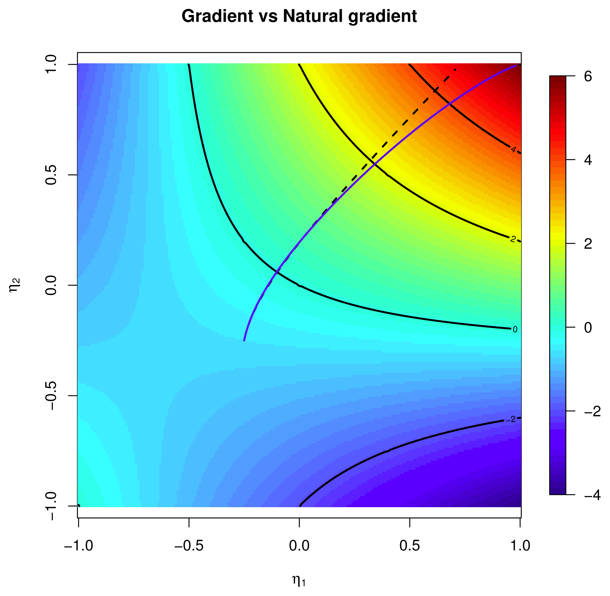
Let us compute the gradient of the relaxed function φ = . [f] : . We have φ_p(θ) = [f], and from the properties of exponential families, the Euclidean gradient is ∇φ_p(0) = Cov_p (f, X). It follows that the natural gradient is:

$$\tilde{\nabla }{\phi }_p(\mathbf{0})=I_{\mathcal{B}}^{-1}(p)\hspace{0.17em}{\text{Cov}}_p(\mathit{X},f)=\widehat{\mathit{f}},$$

(132)

and the Riemannian gradient is ∇φ(p) = F(p).

From the properties of exponential families, we have:

$$\text{Hess\hspace{0.17em}}{\phi }_p(\mathbf{0})={\text{Cov}}_p(\mathit{X},\mathit{X},f),$$

so that, in this case, Equation (127), when written in terms of the moments, is:

$${\mathit{\beta }}^{\prime }\hspace{0.17em}{\text{Cov}}_p(\mathit{X},\mathit{X},f)\hspace{0.17em}\mathit{\alpha }-\frac{1}{2}{\mathit{\beta }}^{\prime }\hspace{0.17em}{\text{Cov}}_p(\mathit{X},\mathit{X},\mathit{\alpha }·\mathit{X})\hspace{0.17em}{\text{Cov}}_p{(\mathit{X},\mathit{X})}^{-1}\hspace{0.17em}{\text{Cov}}_p(\mathit{X},f).$$

(133)

4.1.1. Example: Binary Independent 2.5.2 and 3.2.1 Continued

We list below the computation of the Hessian in the case of two binary independent variables. Computations were done with Sage [22], which allows both the reduction $x_i^2=1$ in the ring of polynomials and the simplifications in the symbolic ring of parameters.

$${\text{Cov}}_{\mathit{\eta }}(\mathit{X},f)=\left(\begin{array}{l}-({\eta }_1^2-1)a_1-({\eta }_1^2{\eta }_2-{\eta }_2)a_{12}\hfill \\ -({\eta }_2^2-1)a_2-({\eta }_1{\eta }_2^2-{\eta }_1)a_{12}\hfill \end{array}\right)=\left(\begin{array}{l}-({\eta }_1-1)({\eta }_1+1)(a_{12}{\eta }_2+a_1)\hfill \\ -({\eta }_2-1)({\eta }_2+1)(a_{12}{\eta }_1+a_2)\hfill \end{array}\right)$$

(134)

$${\text{Cov}}_{\mathit{\eta }}(\mathit{X},\mathit{X})=\left(\begin{array}{rr}\hfill -{\eta }_1^2+1& \hfill 0\\ \hfill 0& \hfill -{\eta }_2^2+1\end{array}\right)=\left(\begin{array}{rr}\hfill -({\eta }_1-1)({\eta }_1+1)& \hfill 0\\ \hfill 0& \hfill -({\eta }_2-1)({\eta }_2+1)\end{array}\right)$$

(135)

$${\text{Cov}}_{\mathit{\eta }}{(\mathit{X},\mathit{X})}^{-1}\hspace{0.17em}{\text{Cov}}_{\mathit{\eta }}(\mathit{X},f)=\left(\begin{array}{c}{a}_{12}{\eta }_2+a_1\\ a_{12}{\eta }_1+a_2\end{array}\right)=\nabla F(\mathit{\eta })$$

(136)

$$\begin{array}{l}{\text{Cov}}_{\mathit{\eta }}(\mathit{X},\mathit{X},f)=\\ \left(\begin{array}{rr}\hfill 2\hspace{0.17em}({\eta }_1^3-{\eta }_1)a_1+2\hspace{0.17em}({\eta }_1^3{\eta }_2-{\eta }_1{\eta }_2)a_{12}& \hfill ({\eta }_1^2{\eta }_2^2-{\eta }_1^2-{\eta }_2^2+1)a_{12}\\ \hfill ({\eta }_1^2{\eta }_2^2-{\eta }_1^2-{\eta }_2^2+1)a_{12}& \hfill 2\hspace{0.17em}({\eta }_1{\eta }_2^3-{\eta }_1{\eta }_2)a_{12}+2\hspace{0.17em}({\eta }_2^3-{\eta }_2)a_2\end{array}\right)=\\ \left(\begin{array}{rr}\hfill 2\hspace{0.17em}({\eta }_1-1)({\eta }_1+1)(a_{12}{\eta }_2+a_1){\eta }_1& \hfill ({\eta }_2-1)({\eta }_2+1)({\eta }_1-1)({\eta }_1+1)a_{12}\\ \hfill ({\eta }_2-1)({\eta }_2+1)({\eta }_1-1)({\eta }_1+1)a_{12}& \hfill 2\hspace{0.17em}({\eta }_2-1)({\eta }_2+1)(a_{12}{\eta }_1+a_2){\eta }_2\end{array}\right)\end{array}$$

(137)

$${\text{Cov}}_{\mathit{\eta }}{(\mathit{X},\mathit{X})}^{-1}\hspace{0.17em}{\text{Cov}}_{\mathit{\eta }}(\mathit{X},\mathit{X},f)=\left(\begin{array}{rr}\hfill -2\hspace{0.17em}(a_{12}{\eta }_2+a_1){\eta }_1& \hfill -a_{12}{\eta }_2^2+a_{12}\\ \hfill -a_{12}{\eta }_1^2+a_{12}& \hfill -2\hspace{0.17em}(a_{12}{\eta }_1+a_2){\eta }_2\end{array}\right)$$

(138)

$${\text{Cov}}_{\mathit{\eta }}(\mathit{X},\mathit{X},\nabla F(\eta ))=\left(\begin{array}{rr}\hfill -2\hspace{0.17em}(a_{12}{\eta }_2+a_1)({\eta }_1+1)({\eta }_1-1){\eta }_1& \hfill 0\\ \hfill 0& \hfill 2\hspace{0.17em}(a_{12}{\eta }_1+a_2)({\eta }_2+1)({\eta }_2-1){\eta }_2\end{array}\right)$$

(139)

$${\text{Cov}}_{\mathit{\eta }}{(\mathit{X},\mathit{X})}^{-1}\hspace{0.17em}{\text{Cov}}_{\mathit{\eta }}(\mathit{X},\mathit{X},\nabla F(\mathit{\eta }))=\left(\begin{array}{rr}\hfill -2\hspace{0.17em}(a_{12}{\eta }_2+a_1){\eta }_1& \hfill 0\\ \hfill 0& \hfill -2\hspace{0.17em}(a_{12}{\eta }_1+a_2){\eta }_2\end{array}\right)$$

(140)

The Riemannian Hessian as a matrix in the basis of the tangent space is:

$$\text{Hess\hspace{0.17em}}F(\mathit{\eta })=\hspace{0.17em}{\text{Cov}}_{\mathit{\eta }}{(\mathit{X},\mathit{X})}^{-1}\left({\text{Cov}}_{\mathit{\eta }}(\mathit{X},\mathit{X},f)-\frac{1}{2}{\text{Cov}}_{\mathit{\eta }}(\mathit{X},\mathit{X},\nabla F(\mathit{\eta }))\right)=\left(\begin{array}{rr}\hfill -(a_{12}{\eta }_2+a_1){\eta }_1& \hfill -a_{12}({\eta }_2+1)({\eta }_2-1)\\ \hfill -a_{12}({\eta }_1+1)({\eta }_1-1)& \hfill -(a_{12}{\eta }_1+a_2){\eta }_2\end{array}\right)$$

(141)

As a check, let us compute the Riemannian Hessian as a natural Hessian in the Riemannian parameters, Hess φ ∘ Exp_p(u) | _u=0; see [4] (Prop. 5.5.4). We have:

$$\begin{array}{l}F\circ {\text{Exp}}_{\mathit{\eta }}(\mathit{u})=a_{12}\hspace{0.17em}\text{sin\hspace{0.17em}}\left(\sqrt{-{\eta }_1^2+1}{u}_1+\text{arcsin\hspace{0.17em}}({\eta }_1)\right)\hspace{0.17em}\text{sin\hspace{0.17em}}\left(\sqrt{-{\eta }_2^2+1}{u}_2+\text{arcsin\hspace{0.17em}}({\eta }_2)\right)+\\ a_1\hspace{0.17em}\text{sin\hspace{0.17em}}\left(\sqrt{-{\eta }_1^2+1}{u}_1+\text{arcsin\hspace{0.17em}}({\eta }_1)\right)+a_2\hspace{0.17em}\text{sin\hspace{0.17em}}\left(\sqrt{-{\eta }_2^2+1}{u}_2+\text{arcsin\hspace{0.17em}}({\eta }_2)\right)\end{array}$$

(142)

and:

$$\begin{array}{l}\text{Hess\hspace{0.17em}}F\circ {\text{Exp}}_{\mathit{\eta }}(\mathit{u}){\mid }_{\mathit{u}=\mathbf{0}}=\\ \left(\begin{array}{rr}\hfill ({\eta }_1^2-1)a_{12}{\eta }_1{\eta }_2+({\eta }_1^2-1)a_1{\eta }_1& \hfill ({\eta }_1^2-1)({\eta }_2^2-1)a_{12}\\ \hfill ({\eta }_1^2-1)({\eta }_2^2-1)a_{12}& \hfill ({\eta }_2^2-1)a_{12}{\eta }_1{\eta }_2+({\eta }_2^2-1)a_2{\eta }_2\end{array}\right)=\\ \left(\begin{array}{rr}\hfill (a_{12}{\eta }_2+a_1)({\eta }_1+1)({\eta }_1-1){\eta }_1& \hfill a_{12}({\eta }_1+1)({\eta }_1-1)({\eta }_2+1)({\eta }_2-1)\\ \hfill a_{12}({\eta }_1+1)({\eta }_1-1)({\eta }_2+1)({\eta }_2-1)& \hfill (a_{12}{\eta }_1+a_2)({\eta }_2+1)({\eta }_2-1){\eta }_2\end{array}\right).\end{array}$$

(143)

Note the presence of the factor Cov_η (X,X).

4.2. Newton Method

The Newton method is an iterative method that generates a sequence of points p_t, with t = 0, 1, . . . , that converges towards a stationary point p̂ of a F(p) = [f], p ∈ , that is, a critical point of the vector field p ↦ ∇F(p), ∇F(p̂) = 0. Here, we follow [4] (Ch. 5–6), and in particular Algorithm 5 on Page 113.

Let ∇F be a gradient field. We reproduce in our case the basic derivation of the Newton method in the following. Note that, in this section, we use the notation Hess •[α] to denote Hess_α •. Using the definition of metric derivative, we have for a geodesic curve [0, 1] ∋ t ↦ p(t) ∈ connecting p = p(0) to p̂ = p(1) that:

$$\frac{d}{dt}{g}_{p(t)}(\nabla F(p(t)),\delta p(t))=g_{p(t)}\hspace{0.17em}(\text{Hess\hspace{0.17em}}F(p(t))[\delta p(t)],\delta p(t))$$

(144)

hence the increment from p to p̂ is:

$$g_{\widehat{p}}(\nabla F(\widehat{p}),\delta p(1))-g_p(\nabla F(p),\delta p(0))={\int }_0^1{g}_{p(t)}\hspace{0.17em}(\text{Hess\hspace{0.17em}}F(p(t))[\delta p(t)],\delta p(t))\mathrm{\hspace{0.17em} }dt.$$

(145)

Now, we assume that ∇F(p̂) = 0 and that in Equation (145), the integral is approximated by the initial value of the integrand, that is to say, the Hessian is approximately constant on the geodesic from p to p̂; we obtain:

$$-g_p\hspace{0.17em}(\nabla F(p),\delta p(0))-g_p(\text{Hess\hspace{0.17em}}F(p)[\delta p(0)],\delta p(0))+∊.$$

(146)

If we can solve the Newton equation:

$$\text{Hess\hspace{0.17em}}F(p(t))[\mathit{u}]=-\nabla F(p)$$

(147)

then u is approximately equal to the initial velocity of the geodesic connecting p to p̂, that is, p̂ = Exp_p(u).

The particular structure of the exponential manifold suggests at least two natural retractions that could be used to move from u to p̂. Namely, we have the Riemannian exponential (θ_t, θ_t+1) ↦ Exp_θt (θ_t+1 – θ_t) and the e-retraction coming from the exponential family itself and defined by (θ_t, θ_t+1) ↦ e_θt (θ_t+1 – θ_t), with θ_t+1 – θ_t = u_t.

In the θ parameters, with the e-retraction, the Newton method generates a sequence (θ_t) according to the following updating rule:

$${\mathit{\theta }}_{t+1}={\mathit{\theta }}_t-\lambda \hspace{0.17em}\text{Hess\hspace{0.17em}}F{({\mathit{\theta }}_t)}^{-1}\tilde{\nabla }F({\mathit{\theta }}_t)$$

(148)

where λ > 0 is an extra parameter intended to control the step size and, in turn, the convergence to θ̂; see [5].

We can rewrite Equation (148) in terms of covariances as:

$${\mathit{\theta }}_{t+1}={\mathit{\theta }}_t-\lambda \hspace{0.17em}{\left({\text{Cov}}_{{\mathit{\theta }}_t}(\mathit{X},\mathit{X},f)-\frac{1}{2}{\text{Cov}}_{{\mathit{\theta }}_t}(\mathit{X},\mathit{X},\tilde{\nabla }F({\mathit{\theta }}_t))\right)}^{-1}\tilde{\nabla }F({\mathit{\theta }}_t).$$

(149)

4.3. Example: Binary Independent

In the η parameters, the Newton step is:

$$\mathit{u}=-\text{Hess\hspace{0.17em}}F{(\mathit{\eta })}^{-1}\nabla F(\mathit{\eta })=\left(\begin{array}{c}\frac{a_{12}^2{\eta }_1+a_{12}{a}_2+(a_1{a}_{12}{\eta }_1+a_1{a}_2){\eta }_2}{a_{12}^2{\eta }_1^2+\left(a_{12}{a}_2{\eta }_1+a_{12}^2\right){\eta }_2^2-a_{12}^2+(a_1{a}_1{\eta }_1^2+a_1{a}_2{\eta }_1){\eta }_2}\\ \frac{a_1{a}_2{\eta }_1+a_1{a}_{12}+(a_{12}{a}_2{\eta }_1+a_{12}^2){\eta }_2}{a_{12}^2{\eta }_1^2+\left(a_{12}{a}_2{\eta }_1+a_{12}^2\right){\eta }_2^2-a_{12}^2+(a_1{a}_{12}{\eta }_1^2+a_1{a}_2{\eta }_1){\eta }_2}\end{array}\right)$$

(150)

and the new η in the Riemannian retraction is:

$${\text{Exp}}_{\mathit{\eta }}(\mathit{u})=\left(\begin{array}{c}\text{sin\hspace{0.17em}}\left(\frac{(a_{12}^2{\eta }_1+a_{12}{a}_2+(a_1{a}_{12}{\eta }_1+a_1{a}_2){\eta }_2)\sqrt{-{\eta }_1^2+1}}{a_{12}^2{\eta }_1^2+(a_{12}{a}_2{\eta }_1+a_{12}^2){\eta }_2^2-a_{12}^2+(a_1{a}_{12}{\eta }_1^2+a_1{a}_2{\eta }_1){\eta }_2}+\text{arcsin\hspace{0.17em}}({\eta }_1)\right)\\ \text{sin}\hspace{0.17em}\left(\frac{(a_1{a}_2{\eta }_1+a_1{a}_{12}+(a_{12}{a}_2{\eta }_1+a_{12}^2){\eta }_2)\sqrt{-{\eta }_2^2+1}}{a_{12}^2{\eta }_1^2+(a_{12}{a}_2{\eta }_1+a_{12}^2)\hspace{0.17em}{\eta }_2^2-a_{12}^2+(a_1{a}_{12}{\eta }_1^2+a_1{a}_2{\eta }_1){\eta }_2}+\text{arcsin\hspace{0.17em}}({\eta }_2)\right).\end{array}\right)$$

(151)

In Figure 6, we represented the vector field associated with the Newton step in the η parameters, with λ = 0.05, using the Riemannian retraction, for the case a₁ = 1, a₂ = 2 and a₁₂ = 3, with:

$${\text{Exp}}_{\mathit{\eta }}(\mathit{u})=\left(\begin{array}{c}\text{sin\hspace{0.17em}}\left(\lambda \frac{\sqrt{-{\eta }_1^2+1}((3\hspace{0.17em}{\eta }_1+2){\eta }_2+9\hspace{0.17em}{\eta }_1+6)}{3\hspace{0.17em}(2\hspace{0.17em}{\eta }_1+3)\hspace{0.17em}{\eta }_2^2+9\hspace{0.17em}{\eta }_1^2+(3\hspace{0.17em}{\eta }_1^2+2\hspace{0.17em}{\eta }_1)\hspace{0.17em}{\eta }_2-9}+\text{arcsin\hspace{0.17em}}({\eta }_1)\right)\\ \text{sin\hspace{0.17em}}\left(\lambda \frac{(3\hspace{0.17em}(2\hspace{0.17em}{\eta }_1+3){\eta }_2+2\hspace{0.17em}{\eta }_1+3)\sqrt{-{\eta }_2^2+1}}{3(2\hspace{0.17em}{\eta }_1+3){\eta }_2^2+9\hspace{0.17em}{\eta }_1^2+(3\hspace{0.17em}{\eta }_1^2+2\hspace{0.17em}{\eta }_1)\hspace{0.17em}{\eta }_2-9}+\text{arcsin\hspace{0.17em}}({\eta }_2)\right)\end{array}\right).$$

(152)

The red dotted lines represented in the figure identify the basins of attraction of the vector field and correspond to the solutions of the explicit equation in η for which the Newton step u is not defined. This vector field can be compared to that in Figure 7, associated with the Newton step for F(η) using the Euclidean geometry. In the Euclidean geometry, F(η) is a quadratic function with one saddle point, so that from any η, the Newton step points in the direction of the critical point. This makes the Newton step unsuitable for an optimization algorithm. On the other side, in the Riemannian geometry, the vertices of the polytope are critical points for F(η), and they determine the presence of multiple basins of attraction, as expected.

Figure 8 shows the Newton step in the θ parameters based on the e-retraction of Equation (149), while Figure 9 represents the Newton step evaluated with respect to the Euclidean geometry. A comparison of the two vector fields shows that, differently from the η parameters, the number of basins of attraction is the same in the two geometries; however, the scale of the vectors is different. In particular, notice how on the plateau, for diverging θ, the Newton step in the Euclidean geometry vanishes, while in the Riemannian geometry, it gets larger. This behavior suggests better convergence properties for an optimization algorithm based on the Newton step evaluated using the proper Riemannian geometry. In the θ parameters, the boundaries of the basins of attraction represented by the red dotted lines have been computed numerically and correspond to the values of θ for which the update step is not defined.

Finally, notice that in both the η and θ parameters, the step is not always in the direction of descent for the function, a common behavior of the Newton method, which converges to the critical points.

5. Discussion and Conclusions

In this paper, we introduced second-order calculus over a statistical manifold, following the approach described in [4], which has been adapted to the special case of exponential statistical models [2,3]. By defining the Riemannian Hessian and using the notion of retraction, we developed the proper machinery necessary for the definition of the updating rule of the Newton method for the optimization of a function defined over an exponential family.

The examples discussed in the paper show that by taking into account the proper Riemannian geometry of a statistical exponential family, the vector fields associated with the Newton step in the different parametrizations change profoundly. Not only new basins of attraction associated with local and global minima appear, as for the expectation parameters, but also the magnitude of the Newton step is affected, as over the plateau in the natural parameters. Such differences are expected to have a strong impact on the performance of an optimization algorithm based on the Newton step, from both the point of view of achievable convergence and the speed of convergence to the optimum.

The Newton method is a popular second order optimization technique based on the computation of the Hessian of the function to be optimized and is well known for its super-linear convergence properties. However, the use of the Newton method poses a number of issues in practice.

First of all, as the examples in Figures 6 and 8 show, the Newton step does not always point in the direction of the natural gradient, and the algorithm may not converge to a (local) optimum of the function. Such behavior is not unexpected; indeed the Newton method tends to converge to critical points of the function to be optimized, which include local minima, local maxima and saddle points. In order to obtain a direction of ascent for the function to be optimized, the Hessian must be negative-definite, i.e., its eigenvalues must be strictly negative, which is not guaranteed in the general case. Another important remark is related to the computational complexity associated with the evaluation of the Hessian, compared to the (natural) gradient. Indeed, to obtain the Newton step d, Christoffel matrices have to be evaluated, together with the third order covariances between sufficient statistics and the function, and the Hessian has to be inverted. Finally, notice that when the Hessian is close to being non-invertible, numerical problems may arise in the computation of the Newton step, and the algorithm may become unstable and diverge.

In the literature, different methods have been proposed to overcome these issues. Among them, we mention quasi-Newton methods, where the update vector is obtained using a modified Hessian, which has been made negative-definite, for instance, by adding a proper correction matrix.

This paper represents the first step in the design of an algorithm based on the Newton method for the optimization over a statistical model. The authors are working on the computational aspects related to the implementation of the method, and a new paper with experimental results is in progress.

References

- Brown, L.D. Fundamentals of Statistical Exponential Families with Applications in Statistical Decision Theory; Number 9 in IMS Lecture Notes. Monograph Series; Institute of Mathematical Statistics: Hayward, CA, USA, 1986; p. 283. [Google Scholar]
- Amari, S.; Nagaoka, H. Methods of Information Geometry; American Mathematical Society: Providence, RI, USA, 2000; p. 206. [Google Scholar]
- Pistone, G. Nonparametric Information Geometry. In Geometric Science of Information; Proceedings of the First International Conference, GSI 2013, Paris, France, 28–30 August 2013, Nielsen, F., Barbaresco, F., Eds.; Lecture Notes in Computer Science, Volume 8085; Springer: Berlin/Heidelberg, Germany, 2013; pp. 5–36. [Google Scholar]
- Absil, P.A.; Mahony, R.; Sepulchre, R. Optimization Algorithms on Matrix Manifolds; Princeton University Press: Princeton, NJ, USA, 2008; p. xvi+224. [Google Scholar]
- Nocedal, J.; Wright, S.J. Numerical Optimization, 2nd ed.; Springer Series in Operations Research and Financial Engineering; Springer: New York, NY, USA, 2006; p. xxii+664. [Google Scholar]
- Do Carmo, M.P. Riemannian geometry; Mathematics: Theory & Applications; Birkhäuser Boston Inc.: Boston, MA, USA, 1992; p. xiv+300. [Google Scholar]
- Abraham, R.; Marsden, J.E.; Ratiu, T. Manifolds, Tensor Analysis, and Applications, 2nd ed; Applied Mathematical Sciences, Volume 75; Springer: New York, NY, USA, 1988; p. x+654. [Google Scholar]
- Lang, S. Differential and Riemannian Manifolds, 3rd ed.; Graduate Texts in Mathematics; Springer: New York, NY, USA, 1995; p. xiv+364. [Google Scholar]
- Pistone, G. Algebraic varieties vs. differentiable manifolds in statistical models. In Algebraic and Geometric Methods in Statistics; Gibilisco, P., Riccomagno, E., Rogantin, M.P., Wynn, H.P., Eds.; Cambridge University Press: Cambridge, UK, 2010. [Google Scholar]
- Malagò, L.; Matteucci, M.; Dal Seno, B. An information geometry perspective on estimation of distribution algorithms: Boundary analysis. Proceedings of the 2008 GECCO Conference Companion On Genetic and Evolutionary Computation (GECCO ’08); ACM: New York, NY, USA, 2008; pp. 2081–2088. [Google Scholar]
- Malagò, L.; Matteucci, M.; Pistone, G. Stochastic Relaxation as a Unifying Approach in 0/1 Programming. Proceedings of the NIPS 2009 Workshop on Discrete Optimization in Machine Learning: Submodularity, Sparsity & Polyhedra (DISCML), Whistler Resort & Spa, BC, Canada, 11–12 December 2009.
- Malagò, L.; Matteucci, M.; Pistone, G. Stochastic Natural Gradient Descent by Estimation of Empirical Covariances. Proceedings of the IEEE Congress on Evolutionary Computation (CEC), New Orleans, LA, USA, 5–8 June 2011; pp. 949–956.
- Malagò, L.; Matteucci, M.; Pistone, G. Towards the geometry of estimation of distribution algorithms based on the exponential family. Proceedings of the 11th Workshop on Foundations of Genetic Algorithms (FOGA ’11), Schwarzenberg, Austria, 5–8 January 2011; ACM: New York, NY, USA, 2011; pp. 230–242. [Google Scholar]
- Malagò, L.; Matteucci, M.; Pistone, G. Natural gradient, fitness modelling and model selection: A unifying perspective. Proceedings of the IEEE Congress on Evolutionary Computation (CEC), Cancun, Mexico, 20–23 June 2013; pp. 486–493.
- Amari, S.I. Natural gradient works efficiently in learning. Neural Comput 1998, 10, 251–276. [Google Scholar]
- Shima, H. The Geometry of Hessian Structures; Scientific Publishing Co Pte. Ltd. World: Hackensack, NJ, USA, 2007; p. xiv+246. [Google Scholar]
- Malagò, L. On the Geometry of Optimization Based on the Exponential Family Relaxation. Ph.D. Thesis, Politecnico di Milano, Milano, Italy, 2012. [Google Scholar]
- Gallavotti, G. Statistical Mechanics: A Short Treatise; Texts and Monographs in Physics; Springer: Berlin, Germany, 1999; p. xiv+339. [Google Scholar]
- Naudts, J. Generalised exponential families and associated entropy functions. Entropy 2008, 10, 131–149. [Google Scholar]
- Esteban, J.; Ray, D. On the Measurement of Polarization. Econometrica 1994, 62, 819–851. [Google Scholar]
- Montalvo, J.; Reynal-Querol, M. Ethnic polarization, potential conflict, and civil wars. Am. Econ. Rev 2005, 796–816. [Google Scholar]
- Stein, W.; et al. Sage Mathematics Software (Version 6.0); The Sage Development Team, 2013. Available online: http://www.sagemath.org (accessed on 27 March 2014).
© 2014 by the authors; licensee MDPI, Basel, Switzerland This article is an open access article distributed under the terms and conditions of the Creative Commons Attribution license (http://creativecommons.org/licenses/by/3.0/).
Share and Cite
Malagò, L.; Pistone, G. Combinatorial Optimization with Information Geometry: The Newton Method. Entropy 2014, 16, 4260-4289. https://doi.org/10.3390/e16084260
Malagò L, Pistone G. Combinatorial Optimization with Information Geometry: The Newton Method. Entropy. 2014; 16(8):4260-4289. https://doi.org/10.3390/e16084260
Chicago/Turabian StyleMalagò, Luigi, and Giovanni Pistone. 2014. "Combinatorial Optimization with Information Geometry: The Newton Method" Entropy 16, no. 8: 4260-4289. https://doi.org/10.3390/e16084260
APA StyleMalagò, L., & Pistone, G. (2014). Combinatorial Optimization with Information Geometry: The Newton Method. Entropy, 16(8), 4260-4289. https://doi.org/10.3390/e16084260