An Estimation of the Entropy for a Rayleigh Distribution Based on Doubly-Generalized Type-II Hybrid Censored Samples

Abstract

In this paper, based on a doubly generalized Type II censored sample, the maximum likelihood estimators (MLEs), the approximate MLE and the Bayes estimator for the entropy of the Rayleigh distribution are derived. We compare the entropy estimators’ root mean squared error (RMSE), bias and Kullback–Leibler divergence values. The simulation procedure is repeated 10,000 times for the sample size n = 10, 20, 40 and 100 and various doubly generalized Type II hybrid censoring schemes. Finally, a real data set has been analyzed for illustrative purposes.

1. Introduction

Let Y be a random variable with a continuous distribution function (cdf) G(y) and a probability density function (pdf) g(y). The differential entropy H(Y) of the random variable is defined by Cover and Thomas [1] to be:

$$H\left(Y\right)=H\left(f\right)=-{\int }_{-\infty }^{\infty }g\left(y\right)\text{log}g\left(y\right)\mathit{dy}.$$

The cdf and pdf of the random variable Y having the Rayleigh distribution are given by:

$$G\left(y;\sigma \right)=1-\text{exp}\left(-\frac{y^2}{2{\sigma }^2}\right),\hspace{0.17em}\hspace{0.17em}\hspace{0.17em}\hspace{0.17em}y>0,\hspace{0.17em}\hspace{0.17em}\hspace{0.17em}\hspace{0.17em}\sigma >0,$$

(1)

and:

$$g\left(y;\sigma \right)=\frac{x}{{\sigma }^2}\text{exp}\hspace{0.17em}\hspace{0.17em}\left(-\frac{y^2}{2{\sigma }^2}\right),\hspace{0.17em}\hspace{0.17em}\hspace{0.17em}y>0,\hspace{0.17em}\hspace{0.17em}\hspace{0.17em}\hspace{0.17em}\sigma >0.$$

(2)

Let Z = Y/σ; then Z has a standard form of the Rayleigh distribution with the cdf written as:

$$\begin{array}{ll}F\left(z\right)\hfill & =1-\text{exp}\left(-\frac{z^2}{2}\right),\hfill \\ f\left(z\right)\hfill & =z\left(1-F\left(z\right)\right).\hfill \end{array}$$

(3)

For the pdf (2), the entropy simplifies to:

$$H\left(f\right)=1+\text{log}\left(\frac{\sigma }{\sqrt{2}}\right)+\frac{\gamma }{2},$$

(4)

where γ is the Euler–Mascheroni constant.

The estimation of the parameters of the censored samples has been investigated by many authors, such as Harter and Moore [2], Dyer and Whisenand [3], Balakrishnan [4], Fernández [5] and Kim and Han [6]. Hater and Moore [2] derived an explicit form of the maximum likelihood estimators (MLEs) of the scale parameter σ based on Type II censored data. Dyer and Whisenand [3] considered the best linear unbiased estimator of σ based on Type II censored data. Balakrishnan [4] considered an approximate MLE of σ based on the doubly generalized Type II censored data. Fernández [5] considered a Bayes estimation of σ based on the doubly-generalized Type II censored data. Recently, Kim and Han [6] considered a Bayes estimation of σ based on the multiply Type II censored data.

In this paper, we derive the estimators for the entropy function of the Rayleigh distribution with an unknown scale parameter under doubly-generalized Type II hybrid censoring. We also compare the proposed estimators in the sense of the root mean squared error (RMSE) for various censored samples.

The rest of this paper is organized as follows. In Section 2, we introduce a doubly generalized Type II hybrid censoring scheme. In Section 3, we describe the computation of the entropy function with MLE and approximate the MLE and Bayes estimator of the unknown scale parameter in the Rayleigh distribution under doubly generalized Type II hybrid censored samples. A real data set has been analyzed in Section 4. In Section 5, the description of different estimators that are compared by performing the Monte Carlo simulation is presented, and Section 6 concludes.

2. Doubly-Generalized Type II Hybrid Censoring Scheme

Consider a life testing experiment in which n units are tested. Epstein [7] introduced a hybrid censoring scheme in which the test is terminated at a random time $T_1^{*}=\text{min}\left\{Y_{r:n},T\right\}$, where r ∈ {1, 2, ···,n}, T ∈ (0, ∞) are pre-fixed and Y_r:n denote the r-th ordered failure time when the sample size is n. Next, Childs et al. [8] introduced a Type I hybrid censoring scheme and a Type II hybrid censoring scheme. The disadvantage of the Type I hybrid censoring scheme is that there is a possibility that very few failures may occur before time T. However, the Type II hybrid censoring scheme can guarantee a pre-fixed number of failures. In this case, the termination point is $T_2^{*}=\text{max}\left\{Y_{r:n},T\right\}$, where r ∈ {1, 2, ···,n} and T ∈ (0, ∞) are pre-fixed. Though the Type II hybrid censored scheme guarantees a pre-fixed number of failures, it might take a long time to observe r failures. In order to provide a guarantee in terms of the number of failures observed, as well as the time to complete the test, Chandrasekar et al. [9] introduced a generalized Type II hybrid censoring scheme.

Lee et al. [10] introduced a doubly generalized Type II hybrid censoring scheme that can be described as follows. Fix 1 ≤ r ≤ n and T₁,T₂,T₃ ∈ (0, ∞), such that T₁ < T₂ < T₃. If the l-th failure occurs before time T₁, start the experiment at T₁; if the l-th failure occurs after time T₁, start at Y_l:n. If the r-th failure occurs before time T₂, terminate the experiment at T₂; if the r-th failure occurs between T₂ and T₃, terminate at Y_r:n; and in other cases, terminate the test at T₃. Therefore, T₁ represents the time at which the researcher starts the observation in the experiment. T₂ represents the least time for which the researcher conducts the experiment. T₃ represents the longest time for which the researcher allows the experiment to continue. 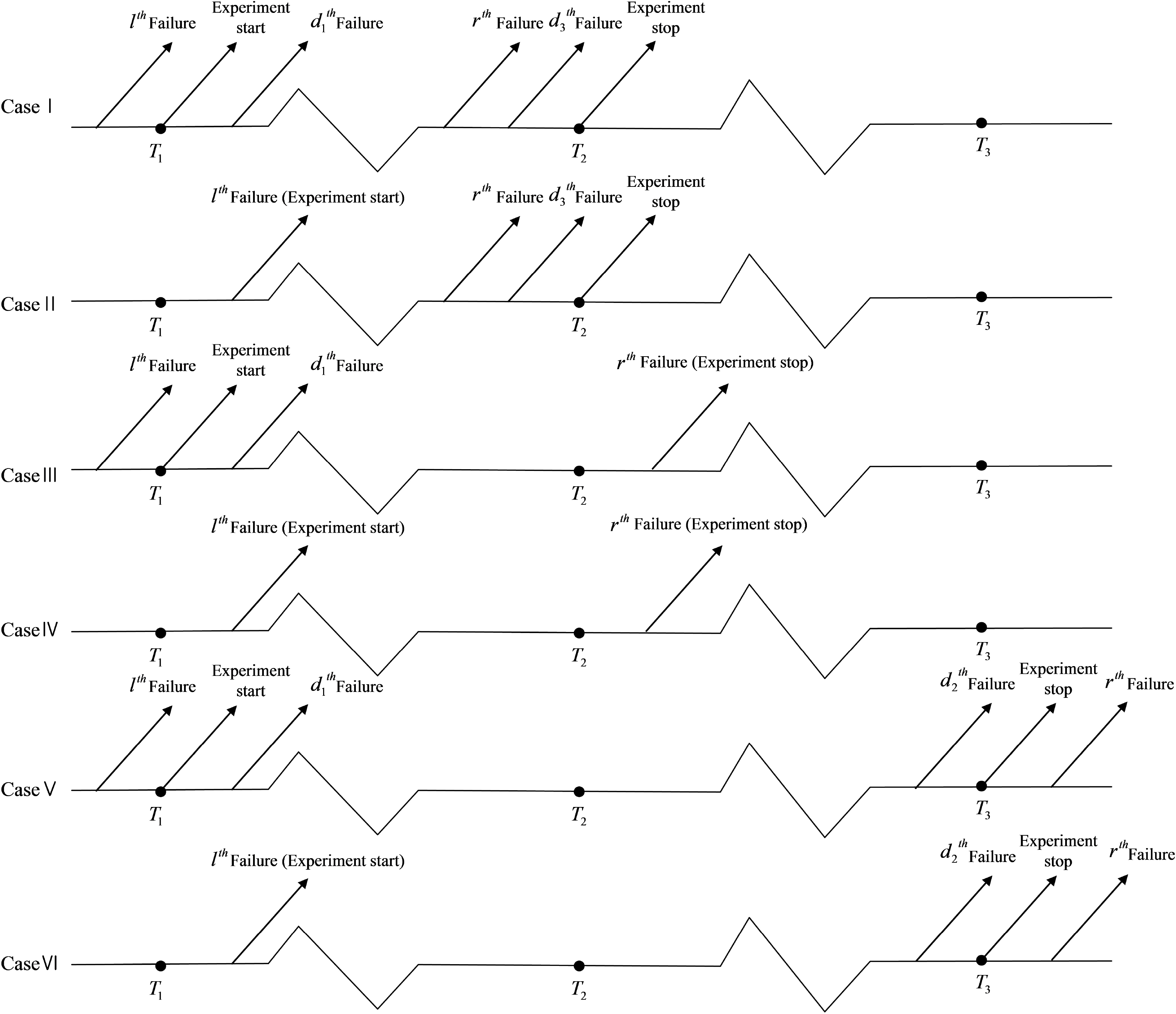For known r, l, T₁, T₂, T₃, we can observe the following six cases of observations.

• Case I : y₁ < ··· <y_l:n < ··· <y_d1−1:n <T₁ <y_d1:n < ··· <y_r:n <y_d3:n <T₂ < ··· <y_d3+1:n, if y_l:n <T₁ and y_r:n <T₂.
• Case II : y₁ < ··· <T₁ < ··· <y_l:n < ··· <y_r:n < ··· <y_d3:n <T₂ <y_d3+1:n, if y_l:n >T₁ and y_r:n <T₂.
• Case III : y₁ < ··· <y_l:n < ··· <y_d1−1:n <T₁ <y_d1:n < ··· <T₂ < ··· <y_r:n, if y_l:n <T₁ and y_r:n >T₂.
• Case IV : y₁ < ··· <T₁ < ··· <y_l:n < ··· <T₂ < ··· <y_r:n, if y_l:n >T₁ and y_r:n >T₂.
• Case V : y₁ < ··· <y_l:n < ··· <y_d1−1:n <T₁ <y_d1:n < ··· <y_d2:n <T₃ <y_d2+1 < ··· <y_r:n, if y_l:n <T₁ and y_r:n >T₃.
• Case VI : y₁ < ··· <T₁ < ··· <y_l:n < ··· <y_d2:n <T₃ <y_d2+1:n < ··· <y_r:n, if y_l:n >T₁ and y_r:n >T₃.

Note that, in Case I, Case III and Case V, we do not observe y_d1−1:n, but y_d1−1:n <T₁ <y_d1:n means that the d₁-th failure took place after T₁, and no failure took place between y_d1:n and T₁. In Case I and Case II, we do not observe y_d3+1:n, but y_d3:n < T₂ < y_d3+1:n means that the d₃-th failure took place before T₂ and no failure took place between y_d3:n and T₂. In Case V and Case VI, we do not observe y_d2+1:n, but y_d2:n < T₃ < y_d2+1:n means that the d₂-th failure took place before T₃, and no failure took place between y_d2:n and T₃. A doubly-generalized Type II hybrid censoring scheme is presented in Figure 1.

3. Estimation of the Entropy

3.1. Maximum Likelihood Estimators

Assume that the failure times of the units are the Rayleigh distribution with cdf (1) and pdf (2). The likelihood functions for six different cases are as follows.

• Case I

  $$L_1\left(\sigma \right)=K_{\text{I}}{\sigma }^{-\left(d_3-d_1+1\right)}{\left[F\left(z_{T_1}\right)\right]}^{d_1-1}{\left[1-F\left(z_{T_2}\right)\right]}^{n-d_3}\prod _{i=d_1}^{d_3}f\left(z_{i:n}\right),$$
• Case II

  $$L_{\text{II}}\left(\sigma \right)=K_{\text{II}}{\sigma }^{-\left(d_3-l+1\right)}{\left[F\left(z_{l:n}\right)\right]}^{l-1}{\left[1-F\left(z_{T_2}\right)\right]}^{n-d_3}\prod _{i=1}^{d_3}f\left(z_{i:n}\right),$$
• Case III

  $$L_{\text{III}}\left(\sigma \right)=K_{\text{III}}{\sigma }^{-\left(r-d_1+1\right)}{\left[F\left(z_{T_1}\right)\right]}^{d_1-1}{\left[1-F\left(z_{r:n}\right)\right]}^{n-r}\prod _{i=d_1}^{r}f\left(z_{i:n}\right),$$
• Case IV

  $$L_{\text{IV}}\left(\sigma \right)=K_{\text{IV}}{\sigma }^{-\left(r-l+1\right)}{\left[F\left(z_{l:n}\right)\right]}^{l-1}{\left[1-F\left(z_{r:n}\right)\right]}^{n-r}\prod _{i=1}^{r}f\left(z_{i:n}\right),$$
• Case V

  $$L_{\text{V}}\left(\sigma \right)=K_{\text{V}}{\sigma }^{-\left(d_2-d_1+1\right)}{\left[F\left(z_{T_1}\right)\right]}^{d_1-1}{\left[1-F\left(z_{T_3}\right)\right]}^{n-d_2}\prod _{i=1}^{d_2}f\left(z_{i:n}\right),$$
• Case VI

  $$L_{\text{VI}}\left(\sigma \right)=K_{\text{VI}}{\sigma }^{-\left(d_2-l+1\right)}{\left[F\left(z_{l:n}\right)\right]}^{l-1}{\left[1-F\left(z_{T_3}\right)\right]}^{n-d_2}\prod _{i=l}^{d_2}f\left(z_{i:n}\right),$$

where K_I = n!/(d₁ − 1)!(n − d₃)!, K_II = n!/(l − 1)!(n − d₃)!, K_III = n!/(d₁ − 1)!(n − r)!, K_IV = n!/(l − 1)!(n − r)!, K_V = n!/(d₁ − 1)!(n − d₂)!, K_VI = n!/(l − 1)!(n − d₂)!, z_T1 = T₁/σ, z_T2 = T₂/σ, and z_T3 = T₃/σ.

Cases I, II, III, IV, V and VI can be combined and be represented as:

$$L\left(\sigma \right)=K{\sigma }^{-A}{\left[F\left(z_{U_1}\right)\right]}^{D_1-1}{\left[1-F\left(z_{U_2}\right)\right]}^{n-D_2}\prod _{i=D_1}^{D_2}f\left(z_{i:n}\right).$$

(5)

Here, U₁ = T₁, U₂ = T₂,D₁ = d₁ and D₂ = d₃ for Case I, U₁ = y_l:n, U₂ = T₂,D₁ = l and D₂ = d₃ for Case II, U₁ = T₁, U₂ = y_r:n,D₁ = d₁ and D₂ = r for Case III, U₁ = y_l:n, U₂ = y_r:n,D₁ = l and D₂ = r for Case IV, U₁ = T₁, U₂ = T₃,D₁ = d₁ and D₂ = d₂ for Case V and U₁ = y_l:n, U₂ = T₃,D₁ = l and D₂ = d₂ for Case VI. Furthermore, z_U1 = U₁/σ, z_U2 = U₂/σ, K = n!/(D₁ − 1)!(n − D₂)! and A = D₂ − D₁ + 1.

From (5), the log-likelihood function can be expressed as:

$$\text{ln}L=-A\text{ln}\sigma +\left(D_1-1\right)\text{ln}F\left(z_{U_1}\right)+\left(n-D_2\right)\text{ln}\left[1-F\left(z_{U_2}\right)\right]+\sum _{i=D_1}^{D_2}\text{ln}f\left(z_{i:n}\right).$$

(6)

On differentiating the log-likelihood function (6) with respect to σ and equating to zero, we obtain the estimating equation:

$$\frac{\partial \text{ln}L}{\partial \sigma }=-\frac{1}{\sigma }\left[2A+\left(D_1+1\right)\frac{f\left(z_{U_1}\right)}{F\left(z_{U_1}\right)}{z}_{U_1}-\left(n-D_2\right)z_{U_2}^2-\sum _{i=D_1}^{D^2}{z}_{i:n}^2\right]=0.$$

(7)

Equation (7) can be solved numerically using the Newton–Raphson method, and an estimate of the entropy function (4) is:

$$\widehat{H}=1+\text{log}\left(\frac{\widehat{\sigma }}{\sqrt{2}}\right)+\frac{\gamma }{2}.$$

3.2. Approximate Maximum Likelihood Estimators

Because the log-likelihood equations cannot be solved explicitly, it will be desirable to consider an approximation to the likelihood equations that will provide explicit estimators of σ. We expand the function f(z_U1)z_U1/F (z_U1) in Taylor series around the points ξ, where $\xi =F^{-1}\left(p\right)=\sqrt{-2\text{ln}\left(q\right)}$, (p) = D₁/(n+ 1) and q = 1−p

We can approximate the functions by:

$$\frac{f\left(z_{U_1}\right)}{F\left(z_{U_1}\right)}{z}_{U_1}\simeq \alpha +\beta z_{U_1},$$

(8)

where:

$$\alpha =\frac{2q\text{ln}q}{p}\left(1+\frac{2\text{ln}q}{p}\right),\hspace{0.17em}\hspace{0.17em}\beta =\frac{2\xi q}{p}\left(1+\frac{\text{ln}q}{p}\right).$$

By substituting Equation (8) into Equation (7), we obtain:

$$\frac{\partial \text{ln}{L}^{*}}{\partial \sigma }=-\frac{1}{\sigma }\left[2A+\left(D_1-1\right)\left(\alpha +\beta z_{U_1}\right)-\left(n-D_2\right)z_{U_2}^2-\sum _{i=D_1}^{D_2}{z}_{i:n}^2\right]=0.$$

(9)

From Equation (9), we obtain σ̂as the solution of the quadratic equation:

$$K{\sigma }^2+B\sigma -C=0,$$

where K = 2A +(D₁ − 1)α > 0, B = (D₁ − 1)βU₁, and $C=(n-D_2)U_2^2+{\sum }_{i=D_1}^{D_2}{y}_{i:n}^2>0$. Therefore,

$${\widehat{\sigma }}_A=\frac{-B+\sqrt{B^2+4KC}}{2K}$$

(10)

is the only positive root.

With σ replaced by the σ̂_A, in Equation (4), the entropy estimators of the Rayleigh distribution based on doubly generalized Type II hybrid censored samples are obtained as:

$${\widehat{H}}_A=1+\text{log}\left(\frac{{\widehat{\sigma }}_A}{\sqrt{2}}\right)+\frac{\gamma }{2}.$$

3.3. Bayes Estimation

In the Bayesian estimation, unknown parameters are assumed to behave as random variables with distributions commonly known as prior probability distributions. In practice, usually, a squared error loss function is taken in to consideration to produce Bayesian estimates. However, under this loss function, overestimation and underestimation are equally penalized, which is not a good criterion from a practical point of view. As an example, in reliability estimation, overestimation is considered to be more serious than the underestimation. Due to such restrictions various asymmetric loss functions are introduced in the literature, such as general entropy loss function. These loss functions have been proven useful for performing Bayesian analysis in different fields of reliability estimation and life testing problems (Rastogi and Tripathi [11]).

A very well-known symmetric loss function is the squared error loss function, which is defined as L₁ d(σ), d̂(σ) = (d̂(σ) − d (σ))² with d̂(σ) being an estimate of d (σ). Here, d (σ) denotes some parametric function of σ. For this situation, the Bayesian estimate, say d̂_S (σ), is given by the posterior mean of d (σ).

One of the most commonly used asymmetric loss function is the general entropy loss given by:

$$L_2\left(d\left(\sigma \right),\widehat{d}\left(\sigma \right)\right)\propto {\left(\frac{\widehat{d}\left(\sigma \right)}{d\left(\sigma \right)}\right)}^q-q\text{log}\left(\frac{\widehat{d}\left(\sigma \right)}{d\left(\sigma \right)}\right)-1,\hspace{0.17em}\hspace{0.17em}\hspace{0.17em}q\ne 0.$$

In this case, the Bayes estimate of d (σ) is obtained as:

$${\widehat{d}}_E\left(\sigma \right)={\left(E_{\sigma }\left({\sigma }^{-q}|x\right)\right)}^{-\frac{1}{q}},$$

provided the above exception exists.

3.3.1. Non-Informative Prior

Since σ based on the doubly generalized Type II censored data is a random variable, we consider the non-informative prior distributions for σ, as:

$${\pi }_1\left(\sigma \right)\propto {\left(\frac{1}{\sigma }\right)}^c.$$

(11)

By combining (5) with (11), the joint density function of σ and Y is given by:

$${\pi }_1\left(\sigma |Y\right)\propto \sum _{j=0}^{D_1-1}\left(\begin{array}{c}{D}_1-1\\ j\end{array}\right){\left(-1\right)}^j{\sigma }^{-\left(2A+c\right)}\text{exp}\left[-\frac{V_1+j{U}_1^2}{2{\sigma }^2}\right],$$

where $V_1=\left(n-D_2\right)U_2^2+{\sum }_{i=D_1}^{D_2}{y}_{i:n}^2$.

Further, the posterior density function of σ is given by:

$${\pi }_1\left(\sigma |Y\right)=\frac{V_1^{A+\left(c-1\right)/2}{\sigma }^{-\left(2A+c-1\right)-1}\text{exp}\left(-\frac{V_1}{2{\sigma }^2}\right){\left[1-\text{exp}\left(\frac{U_1^2}{2{\sigma }^2}\right)\right]}^{D_1-1}}{2^{A+\left(c-3\right)/2}\Gamma \left(A+\left(c-1\right)/2\right){\sum }_{j=0}^{D_1-1}\left(\begin{array}{c}{D}_1-1\\ j\end{array}\right){\left(-1\right)}^j{\left[1+\frac{j{U}_1^2}{V_1}\right]}^{-A-\left(c-1\right)/2}}.$$

Under a squared error loss function, the Bayes estimator of σ is the mean of the posterior density given by:

$${\tilde{\sigma }}_{S_1}=E_1\left[\sigma |Y\right]=\frac{\Gamma \left(A+\left(c-2\right)/2\right){{\sum }_{j=0}^{D_1-1}\left(\begin{array}{c}{D}_1-1\\ j\end{array}\right){\left(-1\right)}^j\left[1+\frac{j{U}_1^2}{V_1}\right]}^{-A\left(c-2\right)/2}}{\Gamma \left(A+\left(c-1\right)/2\right){\sum }_{j=0}^{D_1-1}\left(\begin{array}{c}{D}_1-1\\ j\end{array}\right){\left(-1\right)}^j{\left[1+\frac{j{U}_1^2}{V_1}\right]}^{-A-\left(c-1\right)/2}}{\left(\frac{V_1}{2}\right)}^{1/2}.$$

(12)

Similarly, the Bayes estimator of σ for the general entropy loss function is:

$${\tilde{\sigma }}_{E_1}={\left\{E_1\left[{\sigma }^{-q}|x\right]\right\}}^{-1/q},$$

(13)

where:

$$E_1\left[{\sigma }^{-q}|x\right]=\frac{\Gamma \left(A+\left(c+q-2\right)/2\right){{\sum }_{j=0}^{D_1-1}\left(\begin{array}{c}{D}_1-1\\ j\end{array}\right){\left(-1\right)}^j\left[1+\frac{j{U}_1^2}{V_1}\right]}^{-A\left(c+q-1\right)/2}}{\Gamma \left(A+\left(c-1\right)/2\right){\sum }_{j=0}^{D_1-1}\left(\begin{array}{c}{D}_1-1\\ j\end{array}\right){\left(-1\right)}^j{\left[1+\frac{j{U}_1^2}{V_1}\right]}^{-A-\left(c-1\right)/2}}{\left(\frac{2}{V_1}\right)}^{q/2}.$$

With σ replaced by the σ̃_S1 and σ̃_E1, in Equation (4), the entropy estimator of the Rayleigh distribution based on doubly generalized Type II hybrid censored samples are obtained as:

$${\tilde{H}}_{E_1}=1+\text{log}\left(\frac{{\tilde{\sigma }}_{E_1}}{\sqrt{2}}\right)+\frac{\gamma }{2},\hspace{0.17em}\hspace{0.17em}{\tilde{H}}_{S_1}=1+\text{log}\left(\frac{{\tilde{\sigma }}_{S_1}}{\sqrt{2}}\right)+\frac{\gamma }{2}.$$

3.3.2. Natural Conjugate Prior

Since σ based on the doubly generalized Type II censored data is a random variable, we consider the natural conjugate family of prior distributions for σ that were used by Fernández [5], as:

$${\pi }_2\left(\sigma \right)\propto {\left(\frac{1}{\sigma }\right)}^{2\alpha +1}\hspace{0.17em}\hspace{0.17em}\text{exp}\left(-\frac{\beta }{2{\sigma }^2}\right),\hspace{0.17em}\hspace{0.17em}\hspace{0.17em}\hspace{0.17em}\hspace{0.17em}\sigma >0,$$

(14)

where shape parameter α> 0 and scale parameter β> 0. This is known as the square root inverted gamma density. For β = 0, π(σ) reduces to a general class of improper priors. For α = β = 0, π(σ) reduces to the Jeffreys prior [12].

By combining (5) with (14), the joint density function of σ and Y is given by:

$${\pi }_2\left(\sigma |Y\right)\propto \sum _{j=0}^{D_1-1}\left(\begin{array}{c}{D}_1-1\\ j\end{array}\right){\left(-1\right)}^j{\sigma }^{-\left(2A+2\alpha +1\right)}\text{exp}\left[-\frac{V_2+j{U}_1^2}{2{\sigma }^2}\right],$$

where $V_2=\beta +\left(n-D_2\right)U_2^2+{\sum }_{i=D_1}^{D_2}{y}_{i:n}^2$.

Further, the posterior density function of σ is given by:

$${\pi }_2\left(\sigma |Y\right)=\frac{V_2^{A+\alpha }{\sigma }^{-2{\left(A+\alpha \right)}^{-1}}\text{exp}\left(-\frac{V_2}{2{\sigma }^2}\right){\left[1-\text{exp}\left(\frac{U_1^2}{2{\sigma }^2}\right)\right]}^{D_1-1}}{2^{A+\alpha -1}\Gamma \left(A+\alpha \right){\sum }_{j=0}^{D_1-1}\left(\begin{array}{c}{D}_1-1\\ j\end{array}\right){\left(-1\right)}^j{\left[1+\frac{j{U}_1^2}{V_2}\right]}^{-A-\alpha }}.$$

Under squared error loss function, the Bayes estimator of σ is the mean of the posterior density given by:

$${\tilde{\sigma }}_{S2}=E_2\left[\sigma |Y\right]=\frac{\Gamma \left(A+\alpha -\frac{1}{2}\right){{\sum }_{j=0}^{D_1-1}\left(\begin{array}{c}{D}_1-1\\ j\end{array}\right){\left(-1\right)}^j\left[1+\frac{j{U}_1^2}{V_2}\right]}^{-A-\alpha +\frac{1}{2}}}{\Gamma \left(A+\alpha \right){\sum }_{j=0}^{D_1-1}\left(\begin{array}{c}{D}_1-1\\ j\end{array}\right){\left(-1\right)}^j{\left[1+\frac{j{U}_1^2}{V_1}\right]}^{-A-\alpha }}{\left(\frac{V_2}{2}\right)}^{1/2}.$$

(15)

Similarly, the Bayes estimator of σ for the general entropy loss function is:

$${\tilde{\sigma }}_{E_2}={\left\{E_2\left[{\sigma }^{-q}|x\right]\right\}}^{-1/q},$$

(16)

where:

$$E_2\left[{\sigma }^{-q}|x\right]=\frac{\Gamma \left(A+\alpha +\frac{q}{2}\right){{\sum }_{j=0}^{D_1-1}\left(\begin{array}{c}{D}_1-1\\ j\end{array}\right){\left(-1\right)}^j\left[1+\frac{j{U}_1^2}{V_2}\right]}^{-A-\alpha -\frac{q}{2}}}{\Gamma \left(A+\alpha \right){\sum }_{j=0}^{D_1-1}\left(\begin{array}{c}{D}_1-1\\ j\end{array}\right){\left(-1\right)}^j{\left[1+\frac{j{U}_1^2}{V_2}\right]}^{-A-\alpha }}{\left(\frac{2}{V_2}\right)}^{q/2}.$$

With σ replaced by the σ̃_S2 and σ̃_E2, in Equation (4), the entropy estimators of the Rayleigh distribution based on doubly generalized Type II hybrid censored samples are obtained as:

$${\tilde{H}}_{E_2}=1+\text{log}\left(\frac{{\tilde{\sigma }}_{E_2}}{\sqrt{2}}\right)+\frac{\gamma }{2},\hspace{0.17em}\hspace{0.17em}\hspace{0.17em}\hspace{0.17em}{\tilde{H}}_{S_2}=1+\text{log}\left(\frac{{\tilde{\sigma }}_{S_2}}{\sqrt{2}}\right)+\frac{\gamma }{2}.$$

3.3.3. Bayes Estimation Based on the Balanced Loss Function

From a Bayesian perspective, the choice of loss function is an essential part in the estimation and prediction problems. Recently, a more generalized loss function, called the balanced loss function (Jozani et al.[13]), of the form:

$$L_{\rho ,w,{\delta }_0}\left(\sigma ,\delta \right)=w\rho \left(\delta ,{\delta }_0\right)+\left(1-w\right)\rho \left(\sigma ,\delta \right),$$

(17)

obtained, for instance, using the criterion of MLE, and the weight w takes values in [0,1). Here, ρ is an arbitrary loss function, while δ₀ is a chosen a prior ‘target’ estimator of σ. A general development with regard to Bayesian estimators under L_ρ,w,δ0 is given, namely by relating such estimators to Bayesian solutions to the unbalanced case, i.e., L_ρ,w,δ0 with = 0. L_ρ,w,δ0 can be specialized to various choices of loss function, such as for squared error loss and entropy (Ahmed [14]).

By choosing ρ(σ, δ) = (δ, σ)², Equation (17) reduces to the balanced squared error loss function, in the form:

$$L_{w,{\delta }_0}\left(\sigma ,\delta \right)=w{\left(\delta -{\delta }_0\right)}^2+\left(1-w\right){\left(\delta -\sigma \right)}^2,$$

and the corresponding Bayes estimate of the unknown parameter σ is given by:

$${\delta }_{w,{\delta }_0}\left(y\right)=w{\delta }_0+\left(1+w\right)E\left(\sigma |Y\right).$$

By choosing $\rho \left(\sigma ,\delta \right)={\left(\frac{\sigma }{\delta }\right)}^q-q\text{log}\frac{\sigma }{\delta }-1;$q ≠ 0, Equation (17) reduced to the balanced entropy loss function, in the form:

$$L_{w,{\delta }_0}\left(\sigma ,\delta \right)=w\left\{\frac{{\delta }_0}{\delta }-\text{log}\left(\frac{{\delta }_0}{\delta }\right)-1\right\}+\left(1-w\right)\left\{{\left(\frac{\sigma }{\delta }\right)}^2-\text{log}\left(\frac{\sigma }{\delta }\right)-1\right\},$$

and the corresponding Bayes estimate of the unknown parameter σ is given by:

$${\delta }_{w,{\delta }_0}\left(y\right)={\left\{\frac{w}{{\left({\delta }_0\left(x\right)\right)}^q}+\left(1-w\right)E\left(\frac{1}{{\sigma }^q}\right)\right\}}^{-1/q}.$$

It is clear that the balanced loss functions are more general, which include the maximum likelihood estimate and both symmetric and asymmetric Bayes estimates as special cases.

Based on the balanced squared error loss function, given by Equations (12) and (15), the approximate Bayes estimates of the σ are given, respectively, by:

$${\tilde{\sigma }}_{B{S}_1}=w\widehat{\sigma }+\left(1+w\right){\tilde{\sigma }}_{S_1},\hspace{0.17em}\hspace{0.17em}\hspace{0.17em}{\tilde{\sigma }}_{B{S}_2}=w\widehat{\sigma }+\left(1-w\right){\tilde{\sigma }}_{S_2}.$$

Furthermore, based on the balanced entropy loss function, given by Equations (13) and (16), the approximate Bayes estimates of the σ are given, respectively, by:

$${\tilde{\sigma }}_{B{E}_1}=w\widehat{\sigma }+\left(1+w\right){\tilde{\sigma }}_{E_1},\hspace{0.17em}\hspace{0.17em}\hspace{0.17em}{\tilde{\sigma }}_{B{E}_2}=w\widehat{\sigma }+\left(1-w\right){\tilde{\sigma }}_{E_2}.$$

With σ replaced by the σ̃_BS1, σ̃_BS2, σ̃_BE1 and σ̃_BS2, in Equation (4), the entropy estimators of the Rayleigh distribution based on doubly generalized Type II hybrid censored samples are obtained as:

$${\tilde{H}}_{B{S}_1}=1+\text{log}\left(\frac{{\tilde{\sigma }}_{B{S}_1}}{\sqrt{2}}\right)+\frac{\gamma }{2},\hspace{0.17em}\hspace{0.17em}\hspace{0.17em}\hspace{0.17em}{\tilde{H}}_{B{S}_2}=1+\text{log}\left(\frac{{\tilde{\sigma }}_{B{S}_2}}{\sqrt{2}}\right)+\frac{\gamma }{2},$$

$${\tilde{H}}_{B{E}_1}=1+\text{log}\left(\frac{{\tilde{\sigma }}_{B{E}_1}}{\sqrt{2}}\right)+\frac{\gamma }{2},\hspace{0.17em}\hspace{0.17em}\hspace{0.17em}\hspace{0.17em}{\tilde{H}}_{B{E}_2}=1+\text{log}\left(\frac{{\tilde{\sigma }}_{B{E}_2}}{\sqrt{2}}\right)+\frac{\gamma }{2},$$

4. Illustrative Example

Leiblen and Zelen [15] performed life tests and determined the number of revolutions to failure for 23 ball bearings. The data are doubly generalized Type II hybrid censored data: 23 components were tested. The observed failure times are as follows: 0.1788, 0.2852, 0.3300, 0.4152, 0.4212, 0.4560, 0.4848, 0.5186, 0.5196, 0.5412, 0.5556, 0.6780, 0.6864, 0.6864, 0.6888, 0.8412, 0.9312, 0.9864, 1.0512, 1.0584, 1.2792, 1.2804, 1.7340.

In this example, we assume that the underlying distribution of this data is the Rayleigh distribution based on the doubly generalized Type II hybrid censoring scheme. We take Case I (T₁=0.32, T₂=0.7, T₁=1.2, l=1 and r=17), Case II (T₁=0.32, T₂=0.7, T₁=1.2, l=4 and r=20), Case III (T₁=0.32, T₂=0.7, T₁=1.2, l=7 and r=23), Case IV (T₁=0.64, T₂=0.7, T₁=1.5, l=1 and r=17), Case V (T₁=0.64, T₂=0.7, T₁=1.5, l=3 and r=20) and Case VI (T₁=0.64, T₂=0.7, T₁=1.5, l=7 and r=23). For the Bayesian inference, the prior parameters are chosen (α, β)=(2.0, 2.0) and c = 3. The Bayes estimator based on the natural conjugate prior and non-informative prior is obtained. Furthermore, the Bayes estimator based on the balanced loss function with w = 0.3, 0.5 and 0.7 is obtained.

Table 1. Estimation of entropy for example.

		Complete	Case I	Case II	Case III	Case IV	Case V	Case VI
Ĥ		0.3846	0.3684	0.3479	0.3804	0.3623	0.3404	0.3762
ĤA		0.3846	0.3661	0.3476	0.3804	0.3006	0.2861	0.3312
H̃S1		0.3792	0.3611	0.3416	0.3740	0.3541	0.3335	0.3701
H̃BS1	w = 0.3	0.3808	0.3633	0.3435	0.3759	0.3565	0.3356	0.3719
	w = 0.5	0.3819	0.3648	0.3448	0.3772	0.3582	0.3370	0.3732
	w = 0.7	0.3830	0.3662	0.3460	0.3785	0.3598	0.3383	0.3744
H̃E1		0.3634	0.3398	0.3234	0.3558	0.3323	0.3150	0.3533
H̃BE1	w = 0.3	0.3697	0.3482	0.3307	0.3630	0.3411	0.3225	0.3600
	w = 0.5	0.3739	0.3539	0.3555	0.3679	0.3471	0.3275	0.3646
	w = 0.7	0.3782	0.3597	0.3404	0.3729	0.3531	0.3326	0.3692
H̃S2		0.4204	0.4179	0.3935	0.4216	0.4131	0.3875	0.4148
H̃BS2	w = 0.3	0.4098	0.4033	0.3801	0.4094	0.3981	0.3736	0.4034
	w = 0.5	0.4027	0.3935	0.3710	0.4012	0.3880	0.3642	0.3957
	w = 0.7	0.3955	0.3835	0.3618	0.3929	0.3778	0.3548	0.3880
H̃E2		0.4052	0.3978	0.3762	0.4042	0.3927	0.3699	0.3987
H̃BE2	w = 0.3	0.3989	0.3888	0.3675	0.3969	0.3834	0.3609	0.3919
	w = 0.5	0.3948	0.3829	0.3618	0.3922	0.3772	0.3549	0.3873
	w = 0.7	0.3907	0.3771	0.3562	0.3874	0.3712	0.3491	0.3829

presents estimation of entropy of doubly generalized Type II censoring schemes.

5. Results and Discussion

To compare the performance of the proposed estimators, we simulated the RMSE, bias and Kullback–Leibler divergence of all proposed estimators, by employing the Monte Carlo simulation method. We have used three different doubly generalized Type II hybrid censored sampling schemes, namely: Scheme I: T₁=0.3, T₁=1.7 and T₁=2.0; Scheme II: T₁=0.6, T₁=1.7 and T₁=2.0; and Scheme III: T₁=0.3, T₁=1.7 and T₁=2.3. The doubly generalized Type II hybrid censored samples are generated from the Rayleigh distribution with σ = 1. Using these samples, the RMSE, bias and Kullback–Leibler divergence of entropy estimators are simulated by the Monte Carlo method based on 10,000 runs for the sample size n = 10, 20, 40 and 100. The prior parameters are chosen (α, β) = (2.0, 2.0) and c = 3. The Bayes estimator based on the natural conjugate prior and non-informative prior is obtained. Furthermore, the Bayes estimator based on the balanced loss function with w = 0.3, 0.5 and 0.7 is obtained. The simulation results are presented in Table S1 ∼ Table S10, respectively.

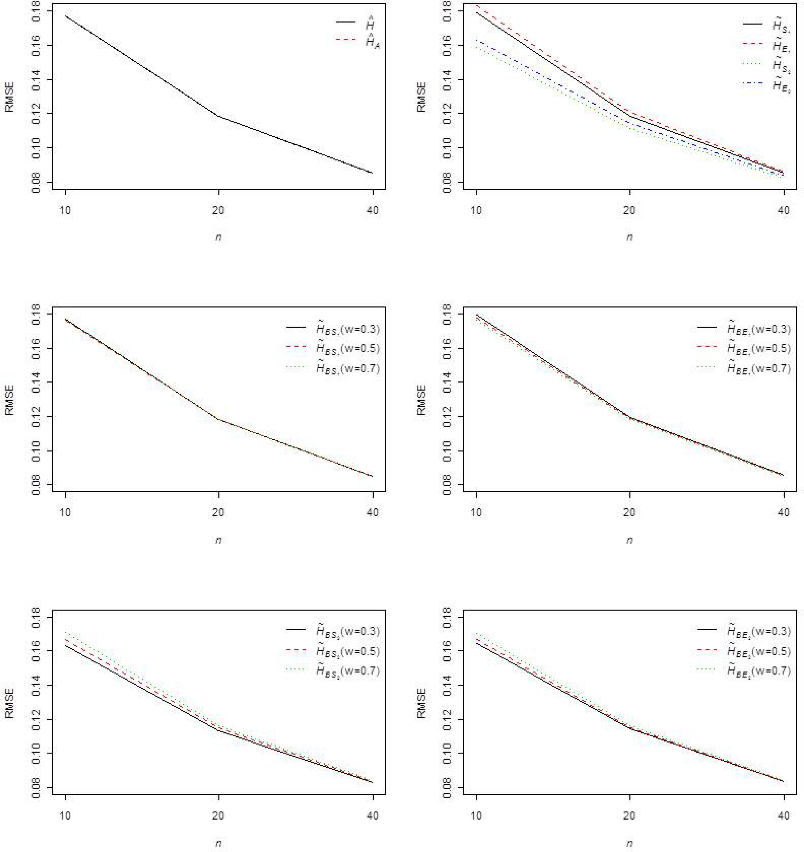
From Table S1 ∼ Table S10, the following general observations can be made. The RMSEs and Kullback–Leibler divergence decrease as sample size n increases. For a fixed sample size, the RMSEs and Kullback–Leibler divergence decrease generally as the number of censored samples decreases. For fixed sample and censored samples size, the RMSEs and Kullback–Leibler divergence decrease generally as the times T₂ and T₃ increases. It is also observed that the left censoring scheme has smaller RMSEs and Kullback–Leibler divergence than the corresponding estimators for right and doubly generalized censoring schemes. For Scheme I and the left censoring case, we presented these in Figure 2.

In Table S1, the average RMSEs and biases of the entropy estimator with MLE and approximate MLE are presented for various choices of n, l, r and censoring schemes. In general, we observed that MLE and approximate MLE behave quite similarly in terms of RMSE. From Table S2 ∼ Table S3, average RMSEs and the bias of the entropy estimator with Bayes estimators based on non-informative prior are presented for various choices of n, l, r and censoring schemes. In general, we observed that entropy estimator with Bayes estimator under the squared error loss function is superior to the respective entropy estimator with Bayes estimator under the general entropy loss function in terms of bias and RMSE. For estimating the entropy, the choice w = 0.7 seems to be a reasonable choice under balanced-square error loss and balanced-entropy loss function. From Table S4 ∼ Table S5, average RMSEs and the biases of the entropy estimator with the Bayes estimator based on the natural conjugate prior are presented for various choices of n, l, r and censoring schemes. In general, we observed that entropy estimator with the Bayes estimator under the squared error loss function is superior to the respective entropy estimator with the Bayes estimator under the general entropy loss function in terms of bias and RMSE. For estimating the entropy, the choice w = 0.3 seems to be a reasonable choice under balanced-square error loss and the balanced-entropy loss function.

In Table S6, the average Kullback–Leibler divergences of the entropy estimator with MLE and approximate MLE are presented for various choices of n, l, r and censoring schemes. In general, we observed that MLE is superior to the respective approximate MLE in terms of Kullback–Leibler divergence. From Table S7 ∼ Table S8, average Kullback–Leibler divergences of the entropy estimator with the Bayes estimator based on the non-informative prior are presented for various choices of n, l, r and censoring schemes. In general, we observed that the entropy estimator with the Bayes estimator under the squared error loss function is superior to the respective entropy estimator with the Bayes estimator under the general entropy loss function in terms of Kullback–Leibler divergence. For estimating the entropy, the choice w = 0.7 seems to be a reasonable choice under balanced square error loss and the balanced entropy loss function. From Table S9 ∼ Table S10, average Kullback–Leibler divergences of the entropy estimator with the Bayes estimator based on the natural conjugate prior are presented for various choices of n, l, r and censoring schemes. In general, we observed that the entropy estimator with the Bayes estimator under the squared error loss function is superior to the respective entropy estimator with the Bayes estimator under the general entropy loss function in terms of the Kullback–Leibler divergence. For estimating the entropy, the choice w = 0.3 seems to be a reasonable choice under the balanced-square error loss and the balanced-entropy loss function. Overall, the Bayes estimator using the squared error loss function based on the natural conjugate prior provide better estimates compared with other estimates.

6. Conclusions

In many life testing experiments, the experimenter may not observe the lifetimes of all inspected units in the life test. Censored data arises in these situations wherein the experimenter does not obtain complete information for all of the units under study. Different types of censoring arise based on how the data are collected from the life testing experiment. In order to provide a guarantee in terms of the number of failures observed, as well as the time to complete the test, Chandrasekar et al. [9] introduced a generalized Type II hybrid censoring scheme. Lee et al. [10] introduced a doubly generalized Type II hybrid censoring scheme, which can handle both right-censoring and left-censoring.

In this paper, we discussed entropy estimators for the Rayleigh distribution based on doubly-generalized Type II hybrid censored samples. The paper derived entropy estimators by using the MLE, approximate MLE and Bayes estimators of the σ in the Rayleigh distribution based on doubly generalized Type II hybrid censored samples and compared them in terms of their RMSE, bias and Kullback–Leibler divergence. Bayesian estimates using the non-informative and natural conjugate prior are obtained under three types of loss function, and it is observed that the Bayes estimate with respect to the natural conjugate prior under the squared error loss function works quite well in this case. Although we focused on the entropy estimate of the Rayleigh distribution in this article, the proposed estimation can be easily extended to other distributions. Particularly, the Bayes estimation can be applied to any other distributions. In contrast, an approximate MLE cannot be simply applied to the distributions with a shape parameter. Estimation on entropy parameters from other distributions is of potential interest in future research.

References

1. Cover, T.M.; Thomas, J.A. Elements of Information Theory; Wiley: Hoboken, NJ, USA, 2005. [Google Scholar]
2. Harter, H.L.; Moore, A.H. Point and interval estimators based on m order statistics for the scale parameter of a Weibull population with known shape parameter. Technometrics 1965, 7, 405–422. [Google Scholar]
3. Dyer, D.D.; Whisenand, C.W. Best linear estimator of the parameter of the Rayleigh distribution-Part I: small sample theory for censored order statistics. IEEE Trans. Reliab 1973, 22, 27–34. [Google Scholar]
4. Balakrishnan, N. Approximate MLE of the scale parameter of the Rayleigh distribution with censoring. IEEE Trans. Reliab 1989, 38, 355–357. [Google Scholar]
5. Fernández, A.J. Bayesian inference from type II doubly censored Rayleigh data. Stat. . Probab. . Lett 2000, 48, 393–399. [Google Scholar]
6. Kim, C.; Han, K. Estimation of the scale parameter of the Rayleigh distribution with multiply type II censored sample. J. Stat. Comput. Simul 2009, 79, 965–976. [Google Scholar]
7. Epstein, B. Truncated life tests in the exponential case. Ann. Math. Stat 1954, 25, 555–564. [Google Scholar]
8. Childs, A.; Chandrasekar, B.; Balakrishnan, N.; Kundu, D. Exact likelihood inference based on type I and type II hybrid censored samples from the exponential distribution. Ann. Inst. Stat. Math 2003, 55, 319–330. [Google Scholar]
9. Chandrasekar, B.; Childs, A.; Balakrishnan, N. Exact likelihood inferance for the exponential distribution under generalized type I and type II hybrid censoring. Nav. Res. Logist 2004, 51, 994–1004. [Google Scholar]
10. Lee, K.; Park, C.; Cho, Y. Inference based on doubly generalized type II hybrid censored sample from a Half Logistic distribution. Commu. Korean Stat. Soc 2011, 18, 645–655. [Google Scholar]
11. Rastogi, M.K.; Tripathi, Y.M. Estimating the parameters of a Burr distribution under progressive type II censoring. Stat. Meth 2012, 9, 381–391. [Google Scholar]
12. Jeffreys, H. Theory of Probability; Clarendon Press: Oxford, UK, 1961. [Google Scholar]
13. Jozani, M.J.; Marchand, E.; Parsian, A. Bayesian and robust Bayesian estimation under a general class of balanced loss function. Stat. Pap 2012, 53, 51–60. [Google Scholar]
14. Ahmed, E.A. Bayesian estimation based on progressive Type II censoring from two-parameter bathtub-shaped lifetime model: an Markov chain Monte Carlo approach. J. Appl. Stat 2014, 41, 752–768. [Google Scholar]
15. Leiblein, J.; Zelen, M. Statistical investigation of the fatigue life of deep-groove ball bearings. J. Res. Nat. Bur. Stand 1952. [Google Scholar]
Figure 1. The doubly generalized Type II hybrid censoring schemes.
Entropy 16 03655f1
Figure 2. The RMSEs of the estimators for Scheme I and left censoring.
Entropy 16 03655f2