Exact Test of Independence Using Mutual Information

Abstract

Using a recently discovered method for producing random symbol sequences with prescribed transition counts, we present an exact null hypothesis significance test (NHST) for mutual information between two random variables, the null hypothesis being that the mutual information is zero (i.e., independence). The exact tests reported in the literature assume that data samples for each variable are sequentially independent and identically distributed (iid). In general, time series data have dependencies (Markov structure) that violate this condition. The algorithm given in this paper is the first exact significance test of mutual information that takes into account the Markov structure. When the Markov order is not known or indefinite, an exact test is used to determine an effective Markov order.

1. Introduction

Mutual information is an information theoretic measure of dependency between two random variables [1]. Unlike correlation, which characterizes linear dependence, mutual information is completely general. The mutual information (in bits) of two discrete random variables X and Y is defined as

$$I(X;Y)={\displaystyle \sum _{x\in X}{\displaystyle \sum _{y\in Y}p(x,y)lo{g}_2}\left(\frac{p(x,y)}{p(x)p(y)}\right).}$$

(1)

Zero dependence occurs if and only if p(x, y) = p(x)p(y); otherwise I(X; Y) is a positive quantity.

In this article we are interested in the case that the marginal and joint probabilities are not known beforehand, but are approximated from data, so that estimates of I(X; Y) will not be exactly zero when X and Y are independent. Thus, in order to make a decision as to whether I(X; Y) > 0, a significance test is necessary. A significance test allows an investigator to specify the stringency for rejection of the null hypothesis I(X; Y) = 0.

The problem of determining significance of dependency can be formulated as a chi-squared test [2] or as an exact test (such as Fisher’s test [3] or permutation tests [4]). The great advantage of exact tests is that they are valid for small datasets; chi-squared tests are only valid in the asymptotic limit of infinite data. Unfortunately, the exact tests reported in the literature assume that consecutive data samples are drawn independently from identical distributions (iid). In general, time series data have dependencies (Markov structure) that violate this condition. In this paper we give the first exact significance test of mutual information that takes into account Markov structure.

2. Testing the Significance of the Null Hypothesis I(X; Y) = 0

To introduce the need for a significance test, suppose the random variables X and Y are the values obtained from the rolls of a pair of six-sided dice, each die independent from the other and equally likely to land on any of its six sides. In the limit of infinite data, the mutual information between X and Y computed using Equation (1) is zero. However, what should we expect for a small number of rolls, say, 75?

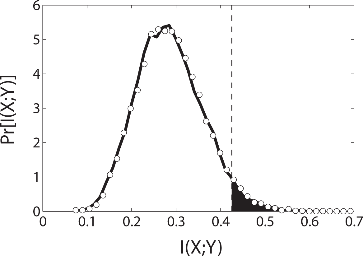
In Figure 1 we plot the result of a numerical simulation of 10, 000 trials of 75 rolls each; the horizontal axis is I(X; Y) and the vertical axis is the probability distribution. The marginals p(x) and p(y) in Equation (1) are estimated by counting the number of occurrences of each of the six symbols {1, 2, 3, 4, 5, 6} for each die and dividing by the total size of the dataset (75). Similarly, the joint probability p(x, y) is obtained by counting the number of occurrences of each of the possible die value pairs, symbols {(1, 1); (1, 2),…, (6, 6)}, divided by the total dataset size. Bias correction is typically employed in practice [7]; however the issue of estimation accuracy is separate from significance testing. The procedure we give here for significance testing is applicable for any choice of bias correction.

The most probable value of mutual information is 0.3 bits/roll, which—if we did not know better—might seem significant considering that the total uncertainty in one die roll is log₂ 6 ≈ 2.585 bits.

The true significance of I, however, can only be determined knowing the distribution I(X; Y) for independent dice (solid line, Figure 1). Knowing this distribution, we would not regard a measurement of I = 0.3 as being significant, since the values of I around 0.3 are, in fact, the most probable to occur when X and Y are independent.

The logic we are describing is that of a null hypothesis significance test (NHST) for mutual information, the null hypothesis being that the mutual information is zero. The probability of obtaining the measured I(X; Y) value, or one larger, is the p-value, and the p-value at which we reject the null hypothesis is the significance level, typically denoted by α A significance level of α = 0.05 means that we reject the null hypothesis if the p-value is less than or equal to 0.05. For the dice example, rejection would occur at I ≥ 0.42 if α = 0.05.

To be clear, the p-value is the probability, assuming the null hypothesis, of the mutual information attaining its observed value or larger. (It is not the probability of the null hypothesis being correct.) While a very small p-value leads one to reject the null hypothesis of independence, a large p-value only implies that the data is consistent with the null hypothesis, not that the null hypothesis should be accepted. In addition, the significance threshold for rejection is entirely up to the investigator to decide.

3. Generating the Mutual Information Distribution from Surrogates

To perform an NHST we need to know the distribution of the test statistic given the null hypothesis. In general, this distribution is not known a priori, but in some cases it can be estimated from the data. Fortunately, the mutual information NHST lends itself to resampling methods [8,9]. Resampling is a procedure that creates multiple datasets—referred to hereafter as surrogates—from the original data. The null hypothesis distribution is extracted from the surrogate data. For an exact NHST, surrogates need to meet two conditions: (1) the null hypothesis must be true for the surrogates; and (2) in every other way they should be like the original data.

In the case of dice, these conditions can be met exactly by randomly permuting the elements of X and Y. Permutation destroys any dependence that may have existed between the datasets but preserves symbol frequencies. Referring to Figure 1, the solid line is the actual distribution of I estimated from 10, 000 trials of 75 data points each. The open circles are the null hypothesis distribution estimated from 10, 000 permutation surrogates of a single time series of 75 data points. We have chosen a data length for which the permutation surrogates recreate the actual distribution well; in contrast, if the original dataset is very small or atypical, the null hypothesis distribution obtained using surrogates will depart from the true distribution.

Also shown in Figure 1 is the significance level, α = 0.05 (dashed line), occurring at approximately I = 0.42. Measured I values that are equal to or greater than 0.42 (shaded region) require rejection of the null hypothesis that the dice are independent. Notice that α = 0.05 implies a five per cent chance of incorrectly rejecting the null hypothesis, known as a Type I error. Lowering the significance level reduces the Type I error rate, but also reduces the sensitivity of the test. In any case, an ideal NHST test will have a Type I error rate equal to the significance level. For the independent die scenario, we repeated the experiment 10, 000 times and found 503 rejections of the null hypothesis, compared with the expected number of rejections 10, 000 × 0.05 = 500.

An equivalent way to compute exact p-values is to create a set of contingency tables and use Fisher’s exact test [3,6]. The elements c_ij of the contingency table are the number of times (x_n, y_n) = (I, j) are observed in the data. Here subscript n is used to indicate x, y pairs that occur at the same time. The table elements, along with the row and column sums, define the joint and marginal probabilities, respectively, and therefore the mutual information I. The probability of obtaining the observed contingency table is equal to the number of possible sequences having the observed contingency table divided by the number of possible sequences having the observed row and column sums. For iid data, the probability of obtaining a particular table is given by the hypergeometric distribution. Finally, the p-value is obtained by summing up the probabilities of all tables with I values equal to or greater than the observed I value.

In this context, counting tables is equivalent to counting sequences with fixed marginals, neither of which is remotely practical except for very small data sets. For the case of 75 rolls of a fair 6-sided die, the number of permutation surrogates is in the order of 10⁵³. In contrast to Fisher’s exact test, the permutation test requires only a uniform sampling from the set of sequences with fixed marginals, rather than a full enumeration. The exact p-value is approximated as the fraction of samples that have mutual information equal to or greater than the observed I. In the limit of infinite surrogate samples the approximated p-value equals the exact p-value. In practice, 10, 000 surrogates are sufficient to perform the NHST when α = 0.05.

4. Accounting for Markov Structure

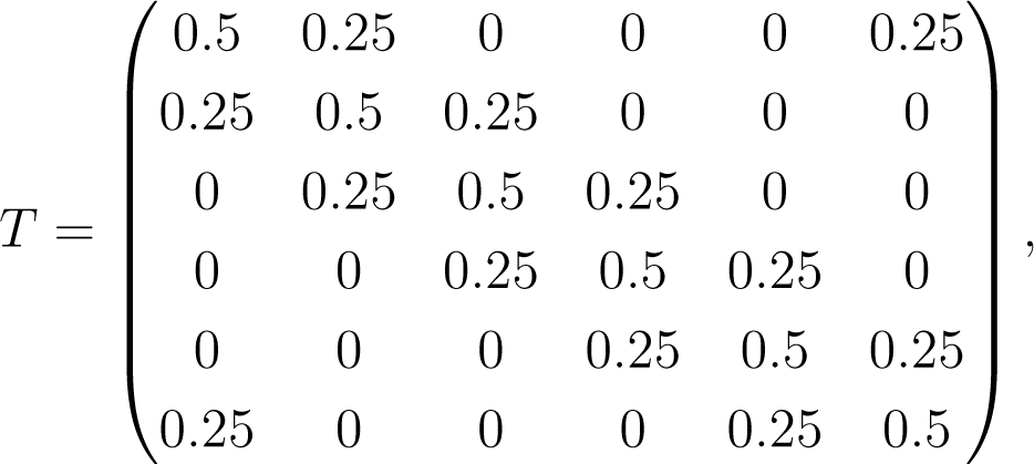
Permutation surrogates preserve single symbol frequencies but not multiple symbol (or word) frequencies. For the dice roll distributions, which are iid, this approach is perfectly adequate, but in general we must take into account that future states may depend on present and past states. For example, let us endow a pair of dice with a Markov property, i.e., the result of the next roll for each die depends probabilistically on its present roll. Suppose we use the following 6 × 6 transition probability matrix for each die:

(2)

where T_ij is the transition probability of going from state i to state j. Inspecting T we see that each die has probability 0.5 of repeating the result of the last roll, probability 0.25 of turning up one higher than the last roll, and 0.25 probability of being one lower. The entropy rate for each Markov die is 1.5 bits/roll.

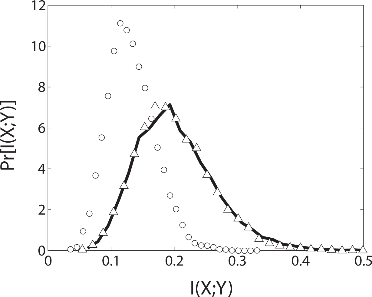
We use simulation to discover the true distribution for I(X; Y) assuming the null hypothesis, this time using 10, 000 trials of 150 rolls each. The results are plotted in Figure 2. As before, the solid line is the true null distribution and the open circles represent the null distribution obtained from permutation surrogates of a single time series. In this case, the permutation distribution, being biased towards smaller values, does not fit the true distribution. Using permutation surrogates, the most probable observed mutual information value (I ≈ 0.2) would lead to an incorrect rejection of the null hypothesis at significance level α = 0.05. This error is due to the fact that the permutation surrogates do not preserve the Markov structure of the original data and thus do not meet the second condition for exactness.

To create an exact test, the surrogates need to be constrained such that not only single symbol counts but also the counts of consecutive symbol pairs are preserved. By preserving the counts of both single and consecutive symbol pairs, the transition probability of the surrogate sequences is made identical to that of the observed sequence.

To be more general, let x^k = x_n, x_n−1,…, x_n−k ∈ X^k+1 denote a (k + 1)-length word and let N(x^k) be the number of such words appearing the data. A surrogate of Markov order k is one that has exactly the same N(x^k) as the original data. A surrogate of Markov order zero is obtained by simple permutation. In the Appendix, we provide an efficient algorithm for producing surrogate sequences with prescribed word counts N(x^k) for any k 0. For an exact test of the I(X; Y) = 0 null hypothesis, the Markov order of the surrogates must match the order of the data.

Knowing that our Markov dice are order one, we generate the correct null hypothesis distribution from surrogates of order one (Figure 2, open triangles). Performing 1000 trials using order-preserving surrogates we found 44 Type I errors, which is in line with the expected number of 1000 × 0.05 = 50. Importantly, the permutation test, which does not preserve Markov order, resulted in 489 Type I errors! Using permutation NHSTs in the presence of Markov structure yields invalid inferences.

The algorithm described in the Appendix can be simply modified to enumerate every sequence of a given Markov order and given marginals. The exact p-value is the fraction of such sequences that have mutual information greater than or equal to the observed I. More usefully, the algorithm can also provide uniform sampling of the set of such sequences so that the first few digits of the exact p-value can be obtained quickly. To the best of our knowledge, this is the only practical method for performing an exact significance test of the null hypothesis that I(X; Y) = 0 when the processes are not iid.

5. Finding the Markov Order

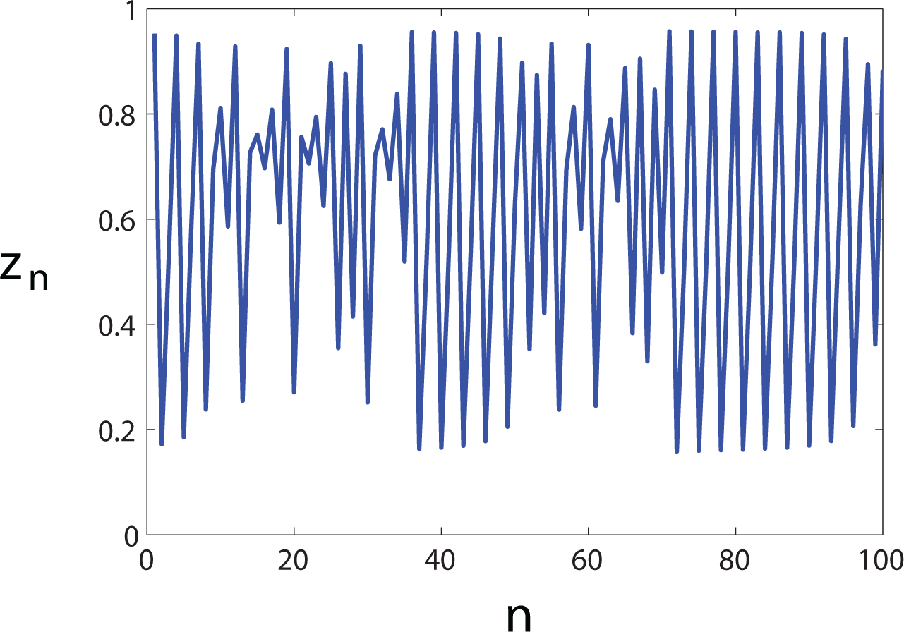
Our algorithm enables the investigator to produce surrogates of a given order but introduces another issue: finding the Markov order of the data. To illustrate, let us take the X and Y processes to be independent instantiations of the logistic map, z_n+1 = rz_n(1 − z_n), where r = 3.827 is in the intermittent chaos regime (Figure 3). For the purpose of computing the mutual information using Equation (1), we partition the interval [0, 1] into 10 equally sized bins and collect statistics from time series of 250 samples. Unlike the previous example, the partitioned logistic map data does not correspond to a Markov process of definite order.

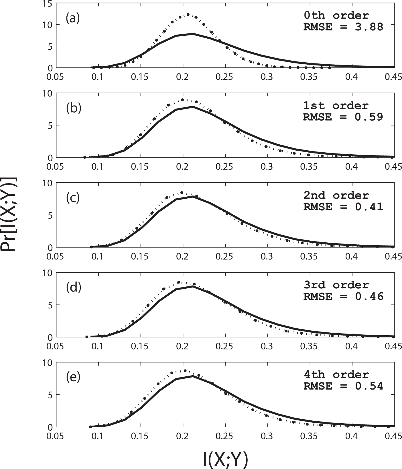
In Figure 4 we plot the distribution of I(X; Y) computed from 10, 000 trials of two independent logistic maps, r = 3.827, 250 iterations per trial (solid line). Subplots (a)–(e) show distribution estimates from surrogates of Markov orders k = 0, 1, 2, 3, 4, respectively (dashed lines).

For the 250-sample logistic map data, the null distribution estimate improves up to order two and then degrades gradually thereafter, based on the root mean square error between the estimated and actual distributions.

What is needed is a method for selecting the optimal order. Fortunately, this is the context in which the order-preserving surrogates were originally developed [5]. In short, to compute the p-value of the null hypothesis that a process is order k, the distribution of a (k + 1)-order test statistic is obtained from an ensemble of order k surrogates. The p-value is the probability of obtaining a test statistic equal to or more extreme than the one observed. A convenient test statistic is the block entropy of the next highest order

$$H_{k+1}={\displaystyle \sum _{x^{k+1}\in X^{k+2}}p}(x^{k+1}){\log }_{2}p(x^{k+1}).$$

(3)

Note that because entropy is reduced by the presence of higher order structure, the p-value is the probability of obtaining a block entropy less than or equal to the observed value. For further explanation, see [5].

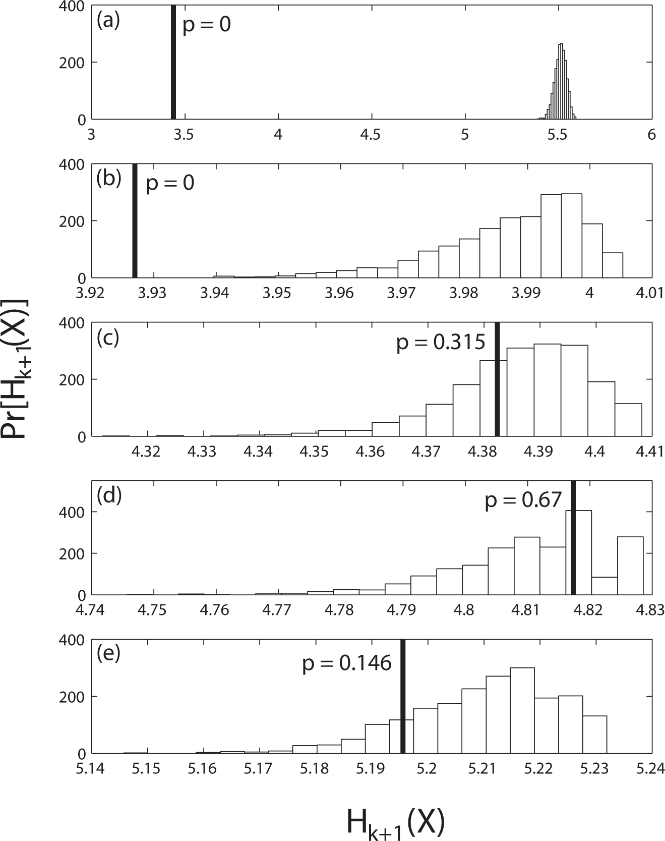
The results of the significance tests for orders k = 0, 1, 2, 3, 4 are shown in Figure 5. The horizontal axes are the block entropies for length k + 2 words. The heavy vertical line indicates the observed block entropy and the bars represent the distribution of the entropies obtained from the surrogates of order k. The p-value, shown next to the vertical line, is the fraction of the surrogate block entropy distribution that lies below the observed block entropy.

Using the standard significance level (α = 0.05), the zeroth and first order hypotheses are rejected, whereas the significance test fails to reject second through fourth order hypotheses. To select an adequate order but prevent over-fitting, we propose choosing the lowest order in which the p-value equals or exceeds the significance level. Note that this test should be performed for each process because different orders may be required for X and Y. In this trial, second order was selected for both processes, but only the X data order tests are shown.

Using this methodology to select the Markov orders, we repeated the exact NHST I(X; Y) = 0, where X and Y are generated from independent logistic maps, 1000 times and found 54 Type I errors, compared with the expected number of 1000 × 0.05 = 50. For the X data, the order test selected second order 576 times, third order 369 times, fourth order 45 times, fifth 8 times, and first and sixth order once each. Because the sampled logistic map data does not have a definite Markov order, the effective order will vary sensitively depending on the sample. In spite of the variation, the above methodology achieves a near ideal Type I error rate.

6. Conclusions

In summary, we have described an exact significance test for I(X; Y) = 0 that can be performed for data of any Markov order. There are two parts: (1) an exact test for selecting the appropriate orders of the X and Y data, and (2) an efficient method for generating order-preserving X and Y surrogates. While a complete enumeration of all order-preserving surrogates is possible (thus giving the exact p-value to all digits), we show how to implement uniform sampling for efficiently determining the first few digits of the p-value. The new method should be used in place of a permutation test any time non-iid data is suspected. We avoided any discussion of entropy bias corrections [7] or bin sizing strategies because these choices do not affect the implementation of the significance test. In the Appendix we give the details of the algorithms needed to generate the order-preserving surrogates.

As a final comment, we wish to point out that this exact test is not sufficient for conditional mutual information quantities, such as transfer entropy [12], although permutation tests are presently being used for this purpose. Permutation tests assume zero mutual information, whereas conditional mutual information quantities can be zero even when mutual information is not. An exact test for conditional mutual information remains an outstanding problem.

References

- Cover, T.M.; Thomas, J.A. Elements of Information Theory; Wiley: New York, NY, USA, 1991. [Google Scholar]
- Greenwood, P.E.; Nikulin, M.S. A Guide to Chi-Squared Testing; Wiley: New York, NY, USA, 1996. [Google Scholar]
- Fisher, R.A. On the interpretation of 2 from contingency tables and the calculation of P. J. R. Stat. Soc 1922, 85, 87–94. [Google Scholar]
- Good, P. Permutation, Parametric, and Bootstrap Tests; Springer: New York, NY, USA, 2005. [Google Scholar]
- Pethel, S.D.; Hahs, D.W. Exact significance test for Markov order. Physica D 2014, 269, 42–47. [Google Scholar]
- Agresti, A. A survey of exact inference for contingency tables. Stat. Sci 1992, 7, 131–153. [Google Scholar]
- Schürmann, T. Bias analysis in entropy estimation. J. Phys. A Math. Gen 2004, 37, L295–L301. [Google Scholar]
- Steuer, R.; Kurths, J.; Daub, C.O.; Weise, J.; Selbig, J. The mutual information: Detecting and evaluating dependencies between variables. Bioinformatics 2002, 18, S231–S240. [Google Scholar]
- Roulston, M. Significance testing of information theoretic functionals. Physica D 1997, 110, 62–66. [Google Scholar]
- Pethel, S.D. Whittle Surrogate. MATLAB Central File Exchange, Available online: http://www.mathworks.com/matlabcentral/fileexchange/40188-whittle-surrogate (accessed on 21 May 2014).
- Billingsley, P. Statistical methods in Markov chains. Ann. Math. Stat 1961, 32, 12–40. [Google Scholar]
- Schreiber, T. Measuring information transfer. Phys. Rev. Lett 2000, 85, 461–464. [Google Scholar]
© 2014 by the authors; licensee MDPI, Basel, Switzerland This article is an open access article distributed under the terms and conditions of the Creative Commons Attribution license (http://creativecommons.org/licenses/by/3.0/).
Share and Cite
Pethel, S.D.; Hahs, D.W. Exact Test of Independence Using Mutual Information. Entropy 2014, 16, 2839-2849. https://doi.org/10.3390/e16052839
Pethel SD, Hahs DW. Exact Test of Independence Using Mutual Information. Entropy. 2014; 16(5):2839-2849. https://doi.org/10.3390/e16052839
Chicago/Turabian StylePethel, Shawn D., and Daniel W. Hahs. 2014. "Exact Test of Independence Using Mutual Information" Entropy 16, no. 5: 2839-2849. https://doi.org/10.3390/e16052839
APA StylePethel, S. D., & Hahs, D. W. (2014). Exact Test of Independence Using Mutual Information. Entropy, 16(5), 2839-2849. https://doi.org/10.3390/e16052839