Application of Entropy and Fractal Dimension Analyses to the Pattern Recognition of Contaminated Fish Responses in Aquaculture


Abstract
:
1. Introduction
2. Materials and Methods
2.1. Experimental Cases
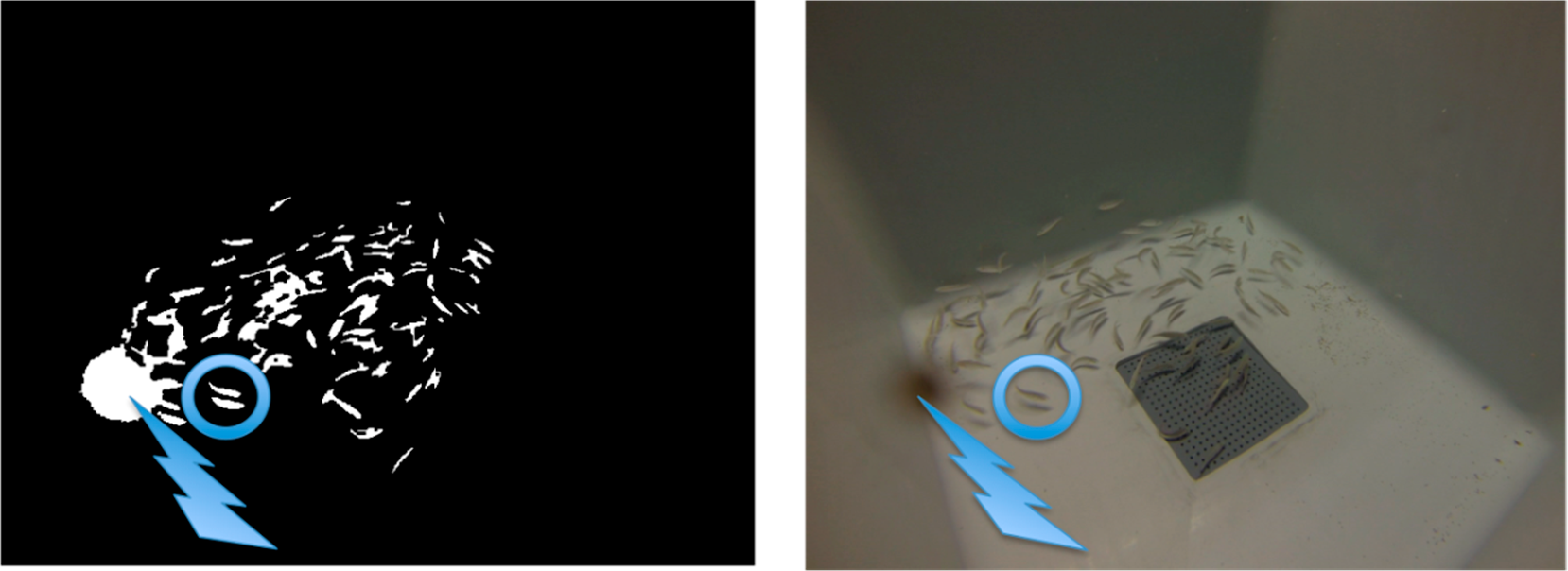
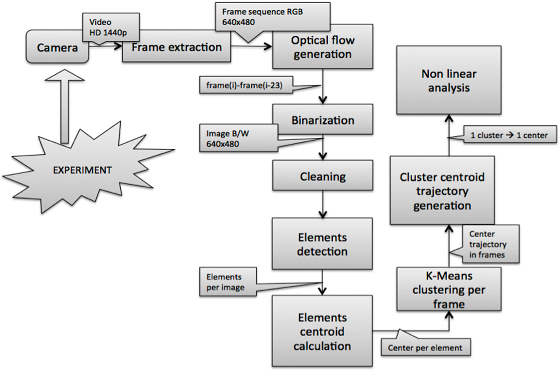
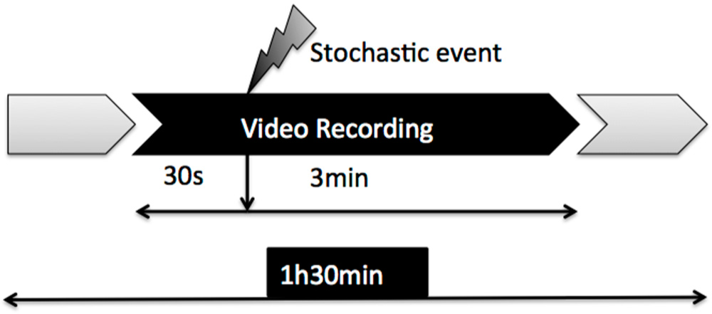
2.2. Image Acquisition and Pre-Processing
2.3. Detection of Objects and Motion Estimation
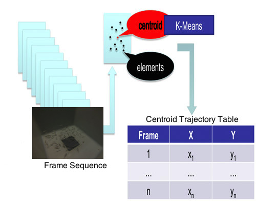
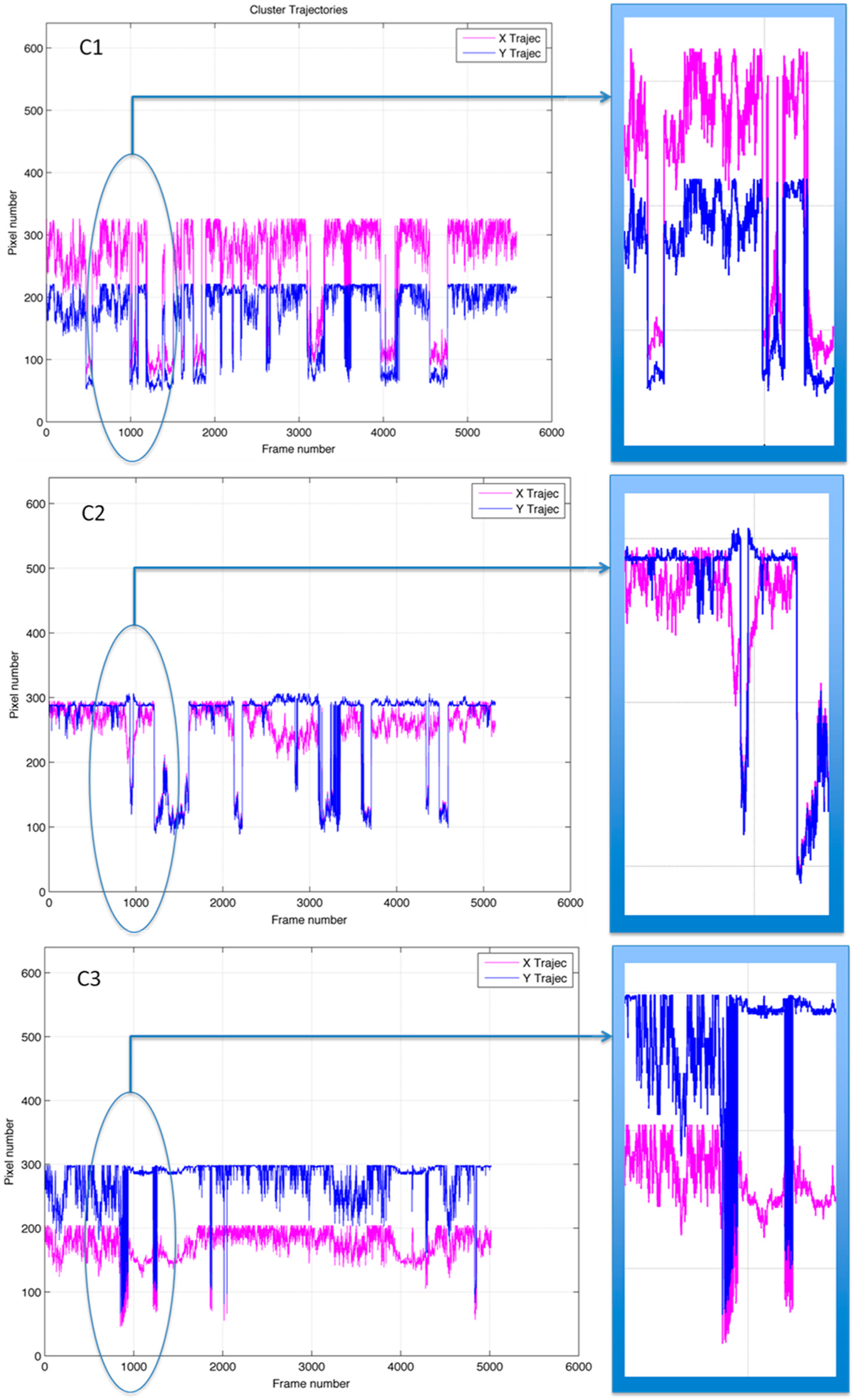
2.4. Clustering and Trajectory Generation
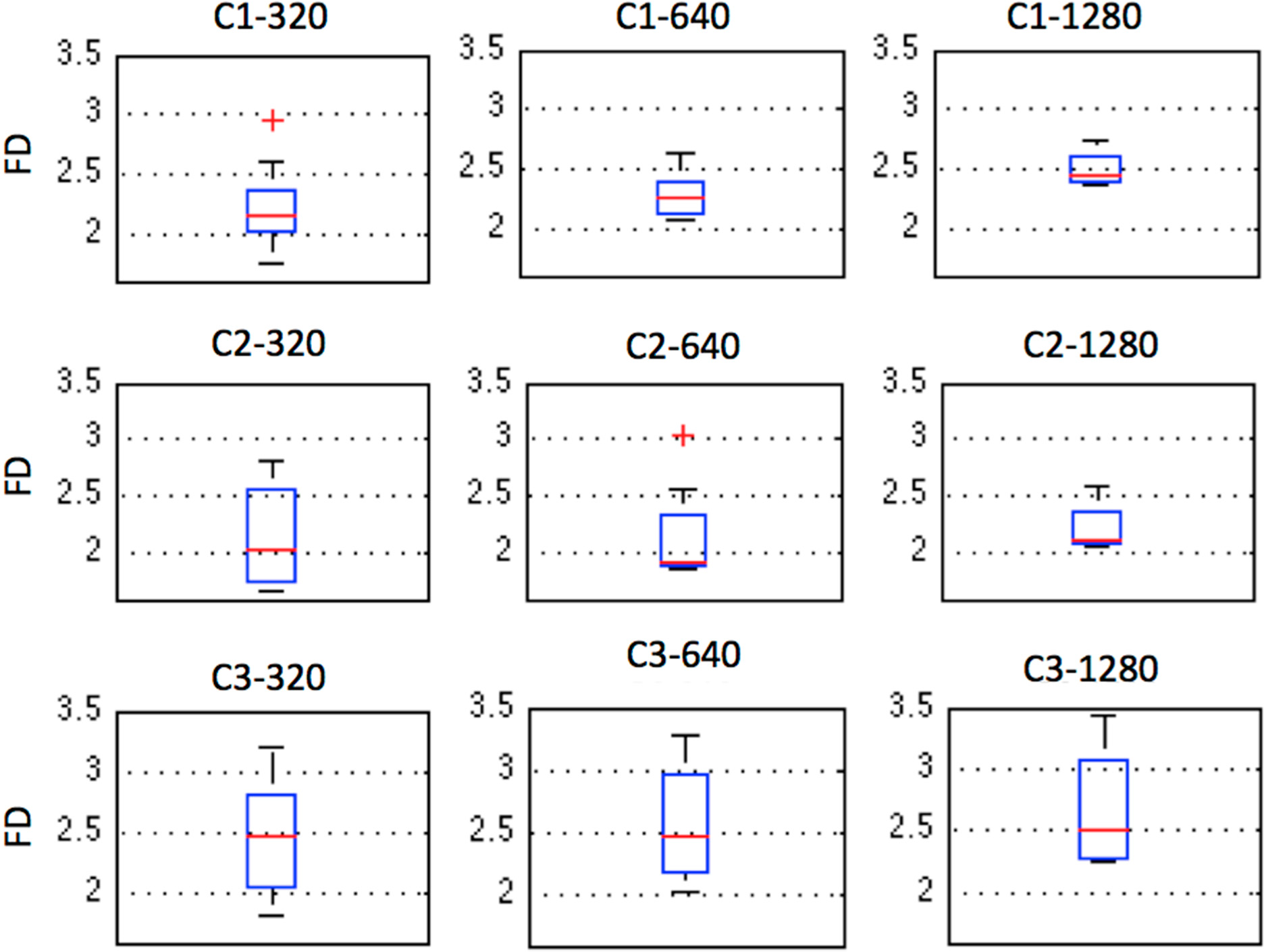
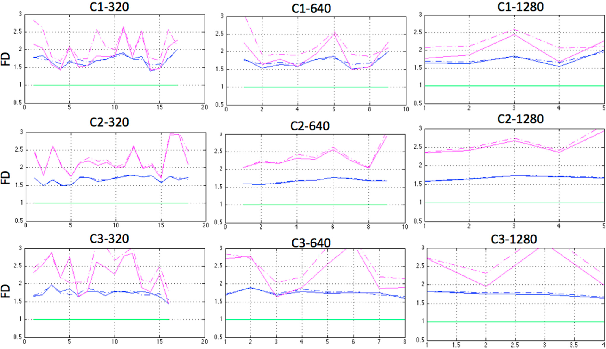
2.5. Fractal Dimension (FD)
2.6. Shannon Entropy
2.7. Permutation Entropy
3. Results and Discussion
4. Conclusions and Future Work
Acknowledgments
Author Contributions
Conflicts of Interest
References
- Kitano, H. Computational systems biology. Nature 2002, 420, 206–210. [Google Scholar]
- Costa, M.; Goldberger, A.; Peng, C.-K. Multiscale entropy analysis of biological signals. Phys. Rev. E 2005, 71, 021906:1–021906:18. [Google Scholar]
- Travieso, C.M.; Alonso, J.B. Special Issue on Advanced Cognitive Systems Based on Nonlinear Analysis. Cogn. Comput. 2013, 5, 397–398. [Google Scholar]
- Spasic, S.; Savi, A.; Nikoli, L.; Budimir, S.; Janoševi, D. Applications of Higuchi’s fractal dimension in the Analysis of Biological Signals. Proceedings of 20th Telecommunications Forum TELFOR 2012, Belgrade, Serbia, 20–22 November 2012; pp. 639–641.
- Accardo, A.; Affinito, M.; Carrozzi, M.; Bouquet, F. Use of the fractal dimension for the analysis of electroencephalographic time series. Biol. Cybern. 1997, 77, 339–350. [Google Scholar]
- Cáceres, J.H.; Sibat Foyaca, H.; Hong, R.; Sautié, M.; Namugowa, A. Towards The Estimation of the Fractal Dimension of Heart Rate Variability Data. Internet J. Cardiovasc. Res. 2004, 2(number 1). [Google Scholar]
- Spasic, S.; Kesic, S.; Kalauzi, A.; Saponjic, J. Different anesthesia in rat induces distinct inter-structure brain dynamic detected by Higuchi fractal dimension. Fractals 2011, 11, 113–123. [Google Scholar]
- Ezeiza, A.; López de Ipiña, K.; Hernández, C.; Barroso, N. Enhancing the Feature Extraction Process for Automatic Speech Recognition with Fractal Dimensions. Cogn. Comput. 2013, 5, 545–550. [Google Scholar]
- Sekine, M.; Tamura, T.; Akay, M.; Fujimoto, T.; Togawa, T.; Fukui, Y. Discrimination of walking patterns using wavelet-based fractal analysis. IEEE Trans. Neural Syst. Rehabil. Eng. 2002, 10, 188–196. [Google Scholar]
- Alados, C.L.; Escos, J.M.; Emlen, J.M. Fractal structure of sequential behaviour patterns: An indicator of stress. Anim. Behav. 1996, 51, 437–443. [Google Scholar]
- Inada, Y.; Kawachi, K. Order and flexibility in the motion of fish schools. J. Theor. Biol. 2002, 214, 371–387. [Google Scholar]
- Tikhonov, D.A.; Enderlein, J.; Malchow, H.; Medvinsky, A.B. Chaos and fractals in fish school motion. Chaos Solitons Fractals 2001, 12, 277–288. [Google Scholar]
- Tikhonov, D.A.; Malchow, H. Chaos and fractals in fish school motion, II. Chaos Solitons Fractals 2003, 16, 287–289. [Google Scholar]
- Kith, K.; Sourina, O.; Kulish, V.; Khoa, N.M. An algorithm for fractal dimension calculation based on Renyi entropy for short time signal analysis. Proceedings of the 7th International Conference on Information, Communications and Signal Processing (ICICS), Macao, China, 7 December 2009; pp. 1–5.
- López-de-Ipiña, K.; Alonso, J.-B.; Travieso, C.M.; Solé-Casals, J.; Eguiraun, H.; Faundez-Zanuy, M.; Ezeiza, A.; Barroso, N.; Ecay-Torres, M.; Martinez-Lage, P.; et al. On the selection of non-invasive methods based on speech analysis oriented to automatic Alzheimer disease diagnosis. Sensors 2013, 13, 6730–6745. [Google Scholar]
- Nimkerdphol, K.; Nakagawa, M. Effect of sodium hypochlorite on zebrafish swimming behavior estimated by fractal dimension analysis. J. Biosci. Bioeng. 2008, 105, 486–492. [Google Scholar]
- Kulish, V.; Sourin, A.; Sourina, O. Human electroencephalograms seen as fractal time series: Mathematical analysis and visualization. Comput. Biol. Med. 2005, 36, 291–302. [Google Scholar]
- Li, X.; Ph, D.; Cui, S.; Voss, L.J. Using permutation entropy to measure the electroencephalographic effects of sevoflurane. Anesthesiology 2008, 109, 448–456. [Google Scholar]
- Liu, Y.; Chon, T.-S.; Baek, H.; Do, Y.; Choi, J.H.; Chung, Y.D. Permutation entropy applied to movement behaviors of Drosophila Melanogaster. Mod. Phys. Lett. B 2011, 25, 1133–1142. [Google Scholar]
- Bandt, C.; Pompe, B. Permutation entropy: A natural complexity measure for time series. Phys. Rev. Lett. 2002, 88, 174102. [Google Scholar]
- Ma, H.; Tsai, T.-F.; Liu, C.-C. Real-time monitoring of water quality using temporal trajectory of live fish. Expert Syst. Appl. 2010, 37, 5158–5171. [Google Scholar]
- Li, D.; Fu, Z.; Duan, Y. Fish-Expert: A web-based expert system for fish disease diagnosis. Expert Syst. Appl. 2002, 23, 311–320. [Google Scholar]
- Li, N.; Wang, R.; Zhang, J.; Fu, Z.; Zhang, X. Developing a knowledge-based early warning system for fish disease/health via water quality management. Expert Syst. Appl. 2009, 36, 6500–6511. [Google Scholar]
- Miaojun, X.; Jianke, Z.; Xiaoqiu, T. Intelligent Fish Disease Diagnostic System Based on SMS Platform. Proceedings of the 3rd International Conference on Intelligent System Design and Engineering Applications, Hong Kong, China, 16–18 January 2013; pp. 897–900.
- Polonschii, C.; Bratu, D.; Gheorghiu, E. Appraisal of fish behaviour based on time series of fish positions issued by a 3D array of ultrasound transducers. Aquac. Eng. 2013, 55, 37–45. [Google Scholar]
- Di Marco, P.; Priori, A.; Finoia, M.G.; Massari, A.; Mandich, A.; Marino, G. Physiological responses of European sea bass Dicentrarchus labrax to different stocking densities and acute stress challenge. Aquaculture 2008, 275, 319–328. [Google Scholar]
- Papoutsoglou, S.; Tziha, G.; Vrettos, X.; Athanasiou, A. Effects of stocking density on behavior and growth rate of European sea bass (Dicentrarchus labrax) juveniles reared in a closed circulated system. Aquac. Eng. 1998, 18, 135–144. [Google Scholar]
- Brodin, T.; Fick, J.; Jonssom, M.; Klaminder, J. Dilute concentrations of a psychiatric drug alter behavior of fish from natural populations. Science 2013, 339, 814–815. [Google Scholar]
- Magnhagen, C.; Braithwaite, V.A.; Forsgren, E.; Kapoor, B.G. Fish Behaviour; Magnhagen, C., Braithwaite, V.A., Forsgren, E., Kapoor, B.G., Eds.; Science Publishers Inc.: Enfield, CT, USA, 2008; p. 646. [Google Scholar]
- Kulish, V.; Sourin, A.; Sourina, O. Analysis and visualization of human electroencephalograms seen as fractal time series. J. Mech. Med. Biol. 2006, 26, 175–188. [Google Scholar]
- Delcourt, J.; Becco, C.; Vandewalle, N.; Poncin, P. A video multitracking system for quantification of individual behavior in a large fish shoal: Advantages and limits. Behav. Res. Methods 2009, 41, 228–235. [Google Scholar]
- Sourina, O.; Sourin, A.; Kulish, V. EEG Data Driven Animation and Its Application. Proceedings of the International Conference Mirage 2009, Rocquencourt, France, 4–6 May 2009; pp. 380–388.
- Brennan, N.P.; Leber, K.M.; Blankenship, H.L.; Ransier, J.M.; DeBruler, R. An Evaluation of Coded Wire and Elastomer Tag Performance in Juvenile Common Snook under Field and Laboratory Conditions. North Am. J. Fish. Manag. 2005, 25, 437–445. [Google Scholar]
- Butail, S.; Chicoli, A.; Paley, D.A. Putting the Fish in the Fish Tank: Immersive VR for Animal Behavior Experiments. Proceedings of the 2012 IEEE International Conference on Robotics and Automation (ICRA), Saint Paul, MN, USA, 14–18 May 2012; pp. 5018–5023.
- Isard, M.; MacCormick, J. BraMBLe: A Bayesian multiple-blob tracker. Proceedings of the 8th IEEE International Conference on Computer Vision (ICCV 2001), Vancouver, BC, Canada, 7–14 July 2001; 2, pp. 34–41.
- Zhao, T.; Nevatia, R. Tracking Multiple Humans in Crowded Environment. Proceedings of the IEEE Conference on Computer Vision and pattern recognition (CVPR 2004), Washington DC, USA, 27 June–2 July 2004; pp. 406–413.
- Isard, M.; Blake, A. Contour tracking by stochastic propagation of conditional density. Proceedings of the European Conference on Computer Vision ECCV, Freiburg, Germany, 2–6 June 1996; pp. 343–356.
- Maccormick, J.; Blake, A. A Probabilistic Exclusion Principle for Tracking Multiple Objects. Int. J. Comput. Vis. 2000, 39, 57–71. [Google Scholar]
- Branson, K.; Belongie, S. Tracking Multiple Mouse Contours (without Too Many Samples). In Proceedings of the 2005. IEEE Computer Society Conference on Computer Vision and Pattern Recognition (CVPR’05), San Diego, CA, USA, 20–25 June 2005; 1, pp. 1039–1046.
- Rasmussen, C.; Hager, G.D. Probabilistic data association methods for tracking complex visual objects. IEEE Trans. Pattern Anal. Mach. Intell. 2001, 23, 560–576. [Google Scholar]
- Sanchez, O.; Dibos, F. Displacement Following of Hidden Objects in a Video Sequence. Int. J. Comput. Vis. 2004, 57, 91–105. [Google Scholar]
- Sigal, L.; Bhatia, S.; Roth, S.; Black, M.J.; Isard, M. Tracking loose-limbed people. In Proceedings of the 2004. IEEE Computer Society Conference on Computer Vision and Pattern Recognition (CVPR 2004), Washington DC, USA, 27 June–2 July 2004; IEEE: Washington DC, USA, 2004; 1, pp. 421–428. [Google Scholar]
- Khan, Z.; Balch, T.; Dellaert, F. MCMC data association and sparse factorization updating for real time multitarget tracking with merged and multiple measurements. IEEE Trans. Pattern Anal. Mach. Intell. 2006, 28, 1960–1972. [Google Scholar]
- Perdomo, D.; Alonso, J.B.; Travieso, C.M.; Ferrer, M.A. Automatic scene calibration for detecting and tracking people using a single camera. Eng. Appl. Artif. Intell. 2013, 26, 924–935. [Google Scholar]
- Barron, J.L.; Fleet, D.J.; Beauchemin, S.S.; Burkitt, T.A. Performance of optical flow techniques. Int. J. Comput. Vis. 1994, 12, 236–242. [Google Scholar]
- Ranchin, F.; Dibos, F. Moving Objects Segmentation Using Optical Flow Estimation. Proceedings of the Workshop on Mathematics and Image Analysis, Paris, France, 6–9 September 2004; pp. 1–18.
- Spath, H. The Cluster Dissection and Analysis Theory FORTRAN Programs Examples; Prentice-Hall, Inc.: Upper Saddle River, NJ, USA, 1985. [Google Scholar]
- Goncalves, W.N.; Monteiro, J.B.O.; de Andrade Silva, J.; Machado, B.B.; Pistori, H.; Odakura, V. Multiple Mice Tracking using a Combination of Particle Filter and K-Means. Proceedings of the XX Brazilian Symposium on Computer Graphics and Image Processing (SIBGRAPI 2007), Belo Horizonte, Brazil, 7–10 October 2007; pp. 173–178.
- Higuchi, T. Approach to an irregular time series on the basis of the fractal theory. Physica D 1988, 31, 277–283. [Google Scholar]
- Katz, M.J. Fractals and the analysis of waveforms. Comput. Biol. Med. 1988, 18, 145–156. [Google Scholar]
- Castiglioni, P. What is wrong in Katz’s method? Comments on: “A note on fractal dimensions of biomedical waveforms”. Comput. Biol. Med. 2010, 40, 950–952. [Google Scholar]
- Tsonis, A. Reconstructing dynamics from observables: The issue of the delay parameter revisited. Int. J. Bifurc. Chaos Appl. Sci. Eng. 2007, 17, 4229–4243. [Google Scholar]
- Mandelbrot, B. How Long is the Coast of Britain? Statistical Self-Similarity and Fractional Dimension Abstract. Science 1965, 156, 636–638. [Google Scholar]
- Esteller, R.; Member, S.; Vachtsevanos, G.; Member, S.; Echauz, J.; Litt, B. A Comparison of Waveform Fractal Dimension Algorithms. IEEE Trans. Circuits Syst. I Fundam. Theory Appl. 2001, 48, 177–183. [Google Scholar]
- Shannon, C.E. A Mathematical Theory of Communication. Bell Syst. Tech. J. 1948. [Google Scholar]
- Shaw, R. Strange Attractors, Chaotic Behavior, and Information Flow. Zeitschrift Für Naturforschung A 1981, 36, 80–112. [Google Scholar]
- Takens, F. Invariants related to dimension and entropy. In Proceedings of the 13th Coloquio Brasileiro de Matematica; Instituto de Matematica Pura e Aplicada: Rio de Janeiro, Brazil, 1983. [Google Scholar]
- Grassberger, P.; Procaccia, I. Measuring the strangeness of strange attractors. In The Theory of Chaotic Attractors; Hunt, B.R., Li, T.-Y., Kennedy, J.A., Nusse, H.E., Eds.; Springer: New York, NY, USA, 2004; pp. 170–189. [Google Scholar]
- Grassberger, P.; Procaccia, I. Estimation of the Kolmogrorov entropy from a chaotic signal. Phys. Rev. A 1983. [Google Scholar]
- Eckmann, J.P.; Ruelle, D. Ergodic theory of chaops and strange attractors. Rev. Mod. Phys. 1985, 57, 617–656. [Google Scholar]
- Pincus, S.M. Approximate entropy as a measure of system complexity. Proc. Natl. Acad. Sci. USA 1991, 88, 2288–2297. [Google Scholar]
- Bandt, C. Ordinal time series analysis. Ecol. Model. 2005, 182, 229–238. [Google Scholar]
- Food and Agriculture Organization (FAO), Report of the Joint FAO/WHO Expert Consultation on the Risks and Benefits of Fish Consumption; FAO Fisheries and Aquaculture Report No. 978; FAO: Rome, Italy, 2010; Volume 978.
- Raghavendra, B.S.; Dutt, D.N. A note on fractal dimensions of biomedical waveforms. Comput. Biol. Med. 2009, 39, 1006–1012. [Google Scholar]
- Fuss, F.K. A robust algorithm for optimisation and customisation of fractal dimensions of time series modified by nonlinearly scaling their time derivatives: Mathematical theory and practical applications. Comput. Math. Methods Med. 2013, 2013, 178476. [Google Scholar]


| Frame Number | X Coordinate | Y Coordinate | Centroid’s Coordinates |
|---|---|---|---|
| 1 | x1 | x | x1,y1 |
| 2 | x2 | y2 | x2,y2 |
| … | … | … | … |
| n | xn | yn | xn,yn |
| Case | Sliding Window Length
| ||
|---|---|---|---|
| 320 | 640 | 1280 | |
| C1 | 2.1415 | 2.2624 | 2.4420 |
| C2 | 2.0449 | 1.9188 | 2.1043 |
| C3 | 2.4752 | 2.4618 | 2.5207 |
| Case | Shannon Entropy Values | Permutation Entropy Values | ||
|---|---|---|---|---|
| X Coordinate | Y Coordinate | X Coordinate | Y Coordinate | |
| C1 | 6.3016 | 6.3016 | 3.0881 | 3.0950 |
| C2 | 6.2861 | 6.2861 | 3.1049 | 3.1250 |
| C3 | 5.3628 | 5.3628 | 3.0413 | 3.0618 |
© 2014 by the authors; licensee MDPI, Basel, Switzerland This article is an open access article distributed under the terms and conditions of the Creative Commons Attribution license (http://creativecommons.org/licenses/by/4.0/).
Share and Cite
Eguiraun, H.; López-de-Ipiña, K.; Martinez, I. Application of Entropy and Fractal Dimension Analyses to the Pattern Recognition of Contaminated Fish Responses in Aquaculture. Entropy 2014, 16, 6133-6151. https://doi.org/10.3390/e16116133
Eguiraun H, López-de-Ipiña K, Martinez I. Application of Entropy and Fractal Dimension Analyses to the Pattern Recognition of Contaminated Fish Responses in Aquaculture. Entropy. 2014; 16(11):6133-6151. https://doi.org/10.3390/e16116133
Chicago/Turabian StyleEguiraun, Harkaitz, Karmele López-de-Ipiña, and Iciar Martinez. 2014. "Application of Entropy and Fractal Dimension Analyses to the Pattern Recognition of Contaminated Fish Responses in Aquaculture" Entropy 16, no. 11: 6133-6151. https://doi.org/10.3390/e16116133
APA StyleEguiraun, H., López-de-Ipiña, K., & Martinez, I. (2014). Application of Entropy and Fractal Dimension Analyses to the Pattern Recognition of Contaminated Fish Responses in Aquaculture. Entropy, 16(11), 6133-6151. https://doi.org/10.3390/e16116133