Article

Global Stability Analysis of a Curzon–Ahlborn Heat Engine under Different Regimes of Performance

by
Israel Reyes-Ramírez
1,*,
Marco A. Barranco-Jiménez
2,*,
Adolfo Rojas-Pacheco
1 and
Lev Guzmán-Vargas
1
1
Unidad Profesional Interdisciplinaria en Ingeniería y Tecnologías Avanzadas, Instituto Politécnico Nacional, Av. IPN 2580, L. Ticomán, México D.F. 07340, Mexico
2
Departamento de Formación Básica, Escuela Superior de Cómputo, Instituto Politécnico Nacional, Av. Miguel Bernard Esq. Juan de Dios Bátiz, U.P. Zacatenco, México D.F. 07738, Mexico
*
Authors to whom correspondence should be addressed.
Entropy 2014, 16(11), 5796-5809; https://doi.org/10.3390/e16115796
Submission received: 27 August 2014 / Revised: 26 October 2014 / Accepted: 29 October 2014 / Published: 4 November 2014
(This article belongs to the Section Thermodynamics)

Abstract

:
We present a global stability analysis of a Curzon–Ahlborn heat engine considering different regimes of performance. The stability theory is used to construct the Lyapunov functions to prove the asymptotic stability behavior around the steady state of internal temperatures. We provide a general analytic procedure for the description of the global stability by considering internal irreversibilities and a linear heat transfer law at the thermal couplings. The conditions of the global stability are explored for three regimes of performance: maximum power (MP), efficient power (EP) and the so-called ecological function (EF). Moreover, the analytical results were corroborated by means of numerical integrations, which fully validate the properties of the global asymptotic stability.

1. Introduction

Since the pioneering paper published by Curzon–Ahlborn in 1975 [1], most of the studies within the context of finite time thermodynamics (FTT) have been centered on steady-state values of characteristic functions, like power output [27], efficient power [8,9], ecological function [10] and saving function [11]. For instance, the Curzon–Ahlborn (CA) engine [1] (see Figure 1) is characterized by the efficiency η = 1 ( T 2 / T 1 ), with T1 > T2, under a maximum power operating regime [1,7,12,13]. However, the energetic description of this kind of model is limited to steady-state situations, with no evident implications for the system’s behavior under dynamical changes [7,14,15]. In 2001, and attending the need of dynamical models of CA-type engines, Santillán et al. [16] introduced for the first time a local stability analysis for CA-engines, reporting an exponential decaying behavior of perturbations about the steady-state internal temperatures. Later, Guzmán-Vargas et al. [17] investigated the effects of the heat transfer laws and the thermal conductance on the CA-engine’s local stability. Páez-Hernández et al. [18] examined the robustness and time delay effects on the performance and stability properties. Barranco-Jiménez et al. [19] studied the local stability of a heat engine, but considering some economic aspects related to the total cost involved in the engine performance. Recently, Reyes-Ramírez et al. [20] investigated the global stability of a CA-engine operating at maximum power output by means of the Lyapunov method. They constructed the Lyapunov function to prove the asymptotic stability behavior about the steady state of the intermediate temperatures in the engine model.
On the other hand, different regimes of performance have been widely studied in the literature in order to characterize the energetic functions of endoreversible engines. Some authors have proposed other maximization criteria, which are quantitatively different compared to the maximum power output; for instance, the minimization of the entropy production, which is represented as the most suitable for the conservation of natural resources. Another regime of performance proposed by Angulo-Brown [10] consists of finding the best trade-off between high power output and low entropy production, this regime is known as the ecological criterion. More recently, Yilmaz [8] proposed a new performance criterion represented by a trade-off between the power output and the efficiency of the system, and it is known as the efficient power regime.
In this work, following the procedure reported in [20], we extend the global stability study considering the other two regimes of performance: maximum efficient power (EP) [8,9] and maximum ecological function (EF) [10]. The work is organized as follows: In Section 2, we explain the main steady-state characteristics of a heat engine model under different regimes of performance. In Section 3, we describe the global stability analysis method based on Lyapunov’s theory to construct the Lyapunov functions for the engine model, both at maximum EP and EF conditions, respectively. In Section 4, we discuss our findings. Finally, in Section 5, we present our conclusions.

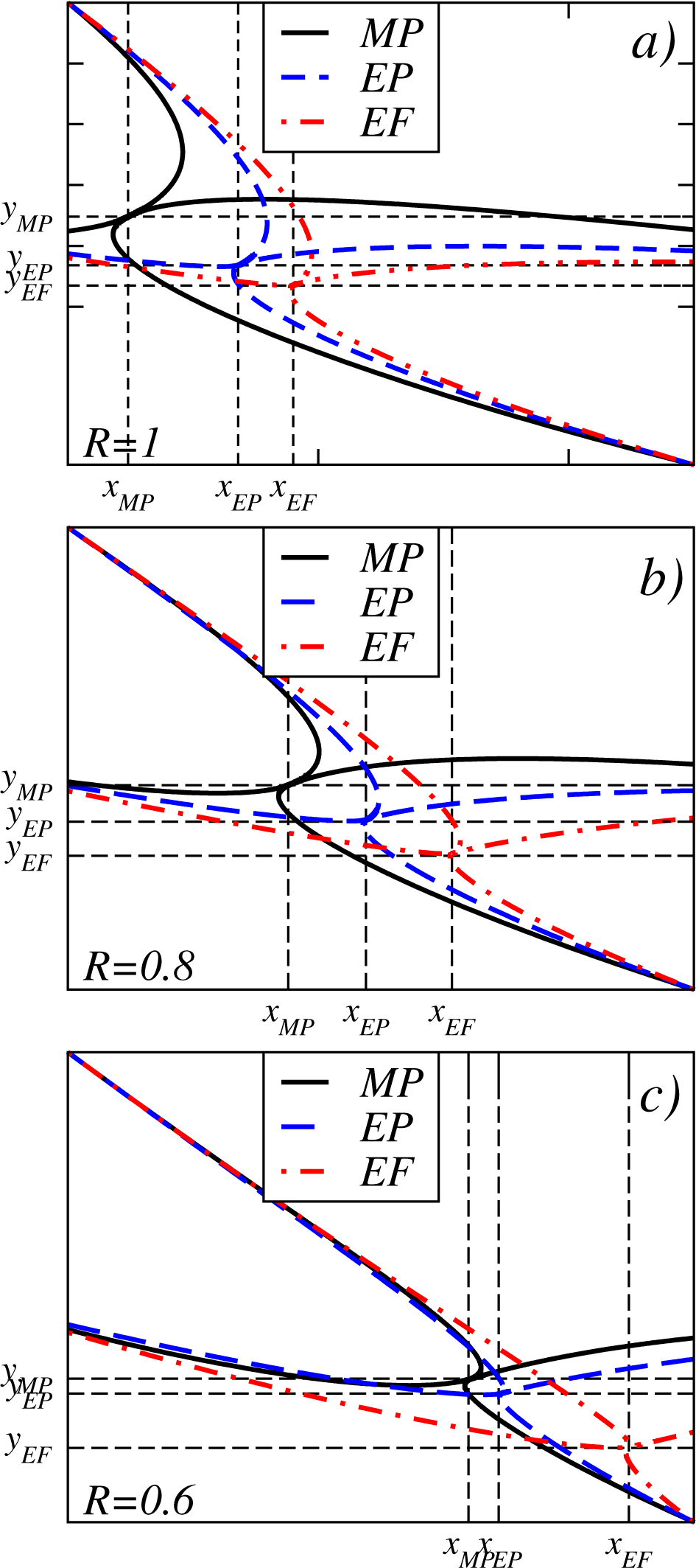
2. Steady-State Characteristics of a Curzon–Ahlborn Engine Model for Different Regimes of Performance

In this section, we present a brief review of the thermodynamical properties of a non-endoreversible Curzon–Ahlborn (CA) heat engine working under different regimes of performance. In Figure 1, a schematic diagram of the irreversible heat engine (CA model) is shown. This engine consists in a Carnot-like thermal engine that works in irreversible cycles and exchanges heat with external thermal reservoirs at temperatures T1 and T2 (T1 > T2). In the steady state, the temperatures of the Carnot-like cycle isothermal branches are x ¯ and y ¯; here, overbars are used to indicate the corresponding steady-state value. Under steady-state conditions, heat flows from the hot reservoir to the internal engine and from the engine to the cold reservoir, which are denoted by J ¯ 1 and J ¯ 2, respectively (see Figure 1). Applying the Clausius theorem and using the fact that the inner Carnot-like engine works in irreversible cycles, we get the following inequality,
J ¯ 1 x ¯ J ¯ 2 y ¯ < 0 ,
This expression can be transformed into an equality by introducing a parameter R leading to [21,22],
J ¯ 1 x ¯ = R J ¯ 2 y ¯ .
The parameter R takes values within the interval 0 < R ≤ 1 (R = 1 corresponds to the endoreversible limit), and it can be seen as a measure of the departure from the endoreversible regime when R < 1 [18,23]. If we assume that the heat flows from T1 to x ¯ and from y ¯ to T2 are of the Newton type, then:
J ¯ 1 = k ( T 1 x ¯ ) ,
J ¯ 2 = k ( y ¯ T 2 ) ,
where κ is the thermal conductance. For simplicity, we have assumed that the heat exchanges take place in conductors with the same thermal conductance κ. The system’s steady-state power output and the efficiency can be defined as,
P ¯ = J ¯ 1 J ¯ 2 ,
and:
η ¯ = P ¯ J ¯ 1 = 1 J ¯ 2 J ¯ 1 = 1 1 R y ¯ x ¯ .
By using Equations (2), (3), (4) and (6), we can write the steady-state temperatures x ¯ and y ¯ and the power output as [17,20],
x ¯ = T 1 1 + R ( 1 + τ 1 η ¯ ) ,
y ¯ = R 1 + R T 1 ( 1 + τ 1 η ¯ ) ( 1 η ¯ ) ,
P ¯ = k T 1 R + 1 η ¯ ( R τ 1 η ¯ ) ,
where τ = T2/T1. The efficiency that maximizes the power output (Equation (9)) is given by [15],
η ¯ M P = 1 τ / R .
It follows that steady-state working temperatures and p the power output can be expressed in terms of τ as follows [18],
x ¯ M P = T 1 1 + R ( 1 + R τ ) ,
y ¯ M P = R 1 + R T 1 ( 1 + R τ ) τ R ,
P ¯ M P = k T 1 R + 1 ( 1 τ R ) ( R R τ ) ,
On the other hand, we can construct the expressions of the efficient power [8,9] and the ecological function [10] following a similar procedure to that used to get Equation (9). Specifically, these functions are given by P ¯ E P = η ¯ P ¯ and E ¯ = P ¯ T 2 σ, respectively, where σ is the total entropy production of the cycle. After a little algebra, we arrive at the following expressions,
P ¯ E P = k T 1 R + 1 η ¯ 2 ( R τ 1 η ¯ ) ,
and:
E ¯ = k T 1 R + 1 ( 2 η ¯ + τ 1 ) ( R τ 1 η ¯ ) ,
where we have applied the second law of thermodynamics to calculate the total entropy production given by σ = J ¯ 2 T 2 J ¯ 1 T 1 (see Figure 1). If we calculate the derivatives of P ¯ E P and E ¯, with respect to η ¯, and solving for the efficiency, we get,
η ¯ E P = 1 τ 4 R τ ( 8 R + τ ) 4 R ,
and:
η ¯ E P = 1 τ ( τ + 1 ) 2 R .
Equations (16) and (17) represent the steady-state efficiencies working under both maximum efficient power ( η ¯ E P ) ([8]) and maximum ecological function conditions ( η ¯ E F ) ([10]), respectively. On the other hand, we can use Equations (6), (10), (16) and (17) to find the expression that relates the internal variables x ¯ and y ¯ to the external temperatures T1 and T2 for the MP, EP and EF cases, to get,
τ M P = y ¯ 2 R x ¯ 2 ,
τ E P = 2 y ¯ 2 x ¯ ( R x ¯ y ¯ ) ,
τ E F = 1 2 [ R x ¯ 2 + 8 y ¯ 2 R x ¯ R x ¯ ] .
The role of the internal temperatures is crucial to perform the stability analysis, and for this reason, T1, T2 and P ¯ must be written in terms of x ¯ and y ¯ [16,17]. In the case of a maximum efficient power regime, we get,
P ¯ E F = k ( R x ¯ y ¯ ) 2 R x ¯ + ( 1 + 2 R ) y ¯ .
Equivalent expressions were obtained for maximum ecological function regime with the help of a symbolic algebra package, but they are quite lengthy to be included.

3. Global Stability Analysis

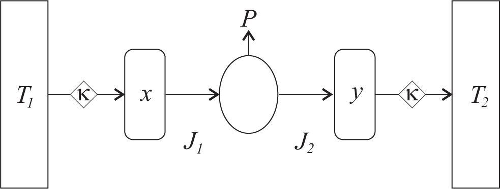
3.1. Dynamical CA-Engine Model

The dynamical model of the CA-engine is based on the rate of change of the internal temperatures, x and y (see Figure 1), that is these temperatures are allowed to change with time, according to the amount of heat entering or exiting [16]. The model assumes that now x and y are considered macroscopic bodies with finite heat capacity C. Thus, the following coupled differential system represents the change of the internal temperatures [16],
x ˙ = 1 C [ k ( T 1 x ) J 1 ] ,
and,
y ˙ = 1 C [ J 2 k ( y T 2 ) ] ,
where J1 and J2 represent the heat flows from the hot reservoir to the internal engine and from the engine to the cold reservoir, respectively. Moreover, assuming that the engine is internally reversible (endoreversible hypothesis), the fluxes J1 and J2, are given by,
J 1 = R x R x y P i ,
and,
J 2 = y R x y P i .
where P represents the power at the regime of performance, with i = MP, EP and EF. We assume that P depends, out of the steady state, on x, y temperatures in a similar way as it depends on x ¯, y ¯.

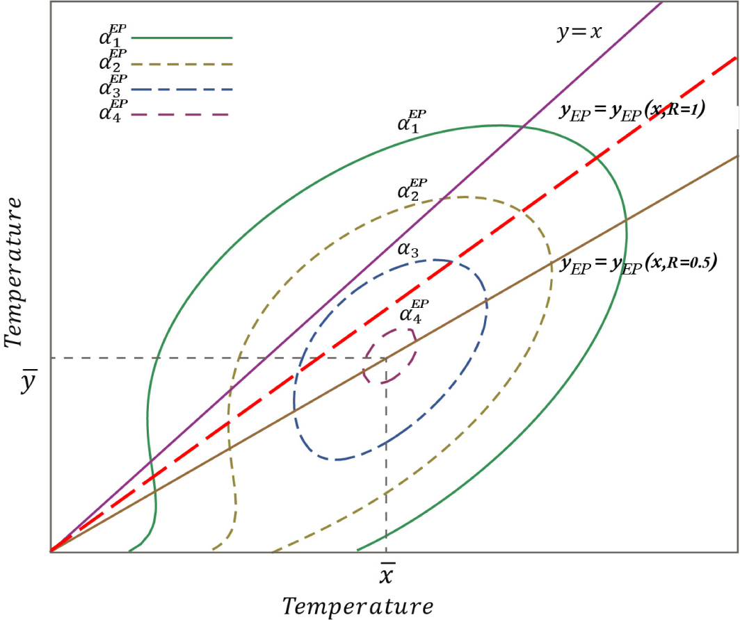
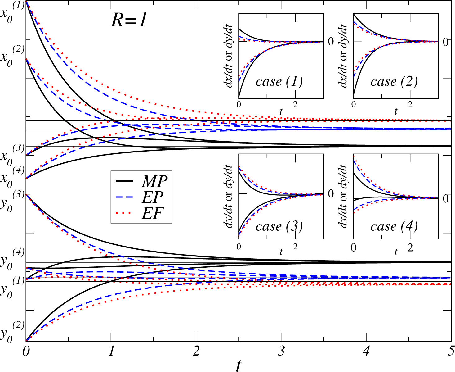
3.2. Lyapunov Functions of the CA-Engine Model under Both Maximum Efficient Power and Maximum Ecological Function

In general, there is not a defined method to find a Lyapunov function, however, a candidate Lyapunov function must satisfy,
  • V (x, y) must be positive definite in a region around the steady state,
  • V ˙ ( x , y ) must be negative definite, that is, V ˙ ( x , y ) 0.
Here, we apply Krasovskii’s method [24] to construct the mentioned Lyapunov functions. This method consists of finding a definite-negative matrix of the form J(X) = A(X) + A+(X), with X = (x, y) and:
A ( X ) = [ f x f y g x g y ] x = x ¯ y = y ¯ ,
being the Jacobian matrix (A+ represents the transpose matrix) and where F (x, y) = (f, g), and ( x ¯ , y ¯ ) is the fixed point of the system. The candidate Lyapunov function is given by [24],
V ( X ) = F ( X ) , F ( X ) = | F ( X ) | 2 .

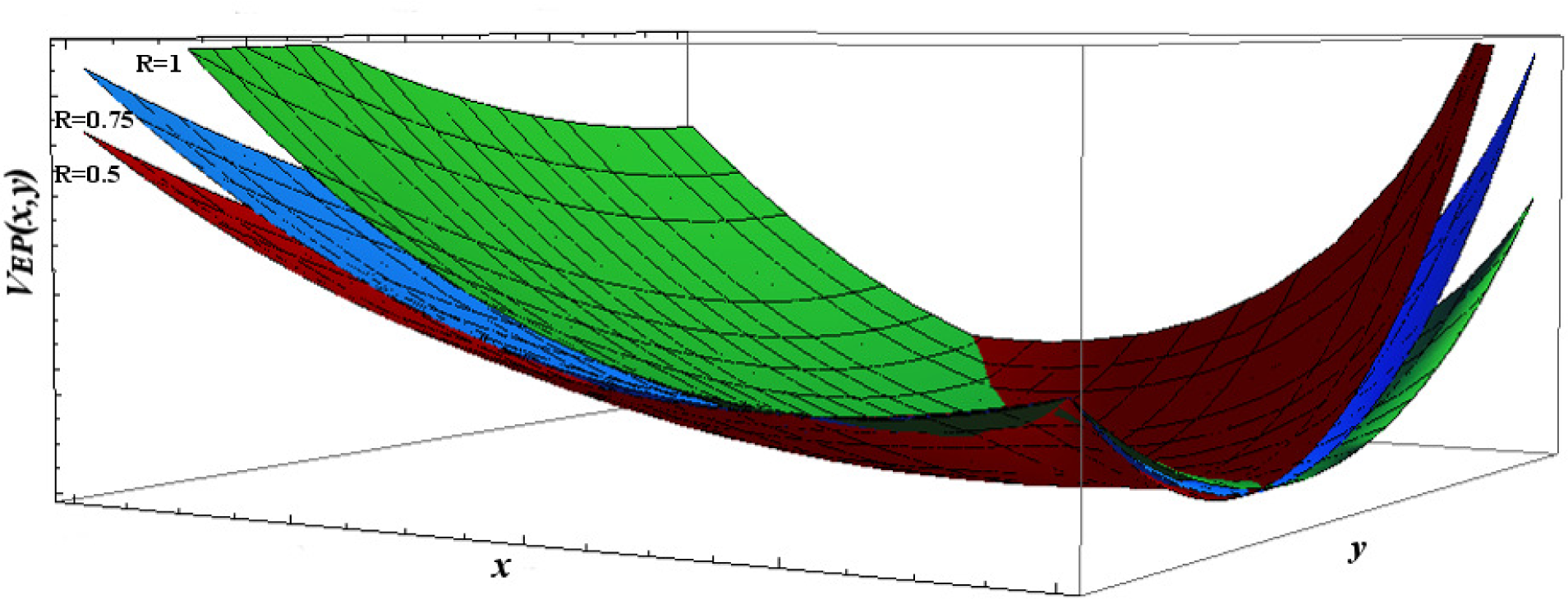
3.3. Maximum Efficient Power Regime

By substituting Equations (21), (24) and (25) into Equations (22) and (23), we get the following dynamic equations for the temperatures x and y under EP conditions,
x ˙ E P = k C [ ( T 1 x ) R x R x + ( 1 + 2 R ) y ( y R x ) ] ,
and:
y ˙ E P = k C [ y R x + ( 1 + 2 R ) y ( y R x ) ( y T 2 ) ] .
These equation systems are of the form x ˙ = f ( x , y ), y ˙ = f ( x , y ), and have a fixed point at ( x ¯ , y ¯ ), that is, f ( x ¯ , y ¯ ) = 0 and g ( x ¯ , y ¯ ) = 0. Following a similar procedure of [20], we construct the matrix J(X),
J E P = 2 k C ( 1 + R ) R 1 ( 1 + τ R + 2 τ R ) 2 [ λ 1 ( R , τ ) R ( 1 + τ ) R ( 1 + τ ) λ 2 ( R , τ ) ] ,
where λ 1 ( R , τ ) = τ + R ( 1 + 2 τ ) + 2 R τ ( 1 + 2 R ) and λ 2 ( R , τ ) = 2 τ + 4 R τ ( 1 + R τ ). Due to the fact that the matrix JEP is definite negative, as we can easily verify, the candidate Lyapunov function for the CA-engine model at maximum efficient power is of the form,
V E P ( x , y ) = k 2 C 2 [ ( T 1 x R x ( y R x ) y + R ( x + 2 y ) ) 2 + ( T 2 y + y ( y R x ) y + R ( x + 2 y ) ) 2 ] .
From the previous equation, as in the case of maximum power conditions [20], we can verify that V E P ( x ¯ , y ¯ ) = 0, that is the steady-state regime is the extremum and global minimum of VEP (x, y). Besides, the previous equation satisfies,
V ˙ E P ( x , y ) = V E P x x ˙ + V E P y y ˙ = V E P , X ˙ 0.

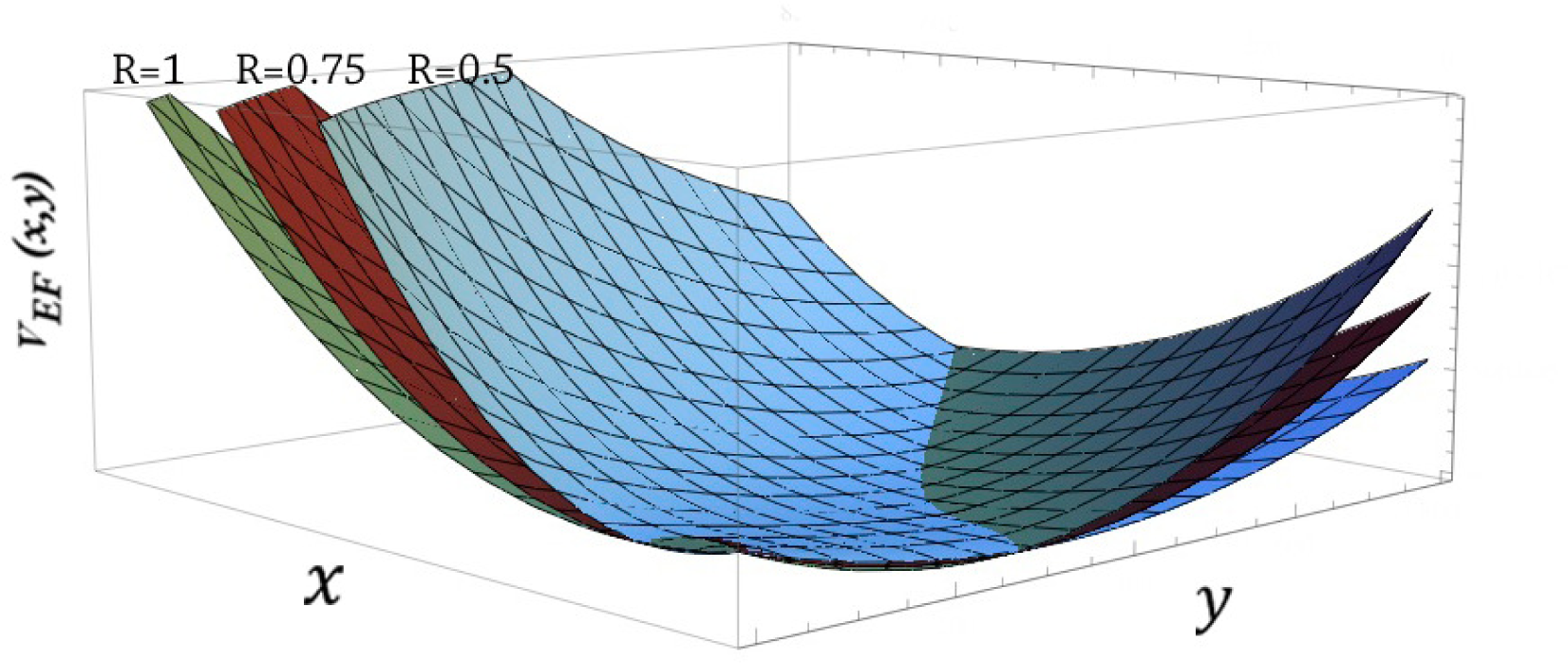
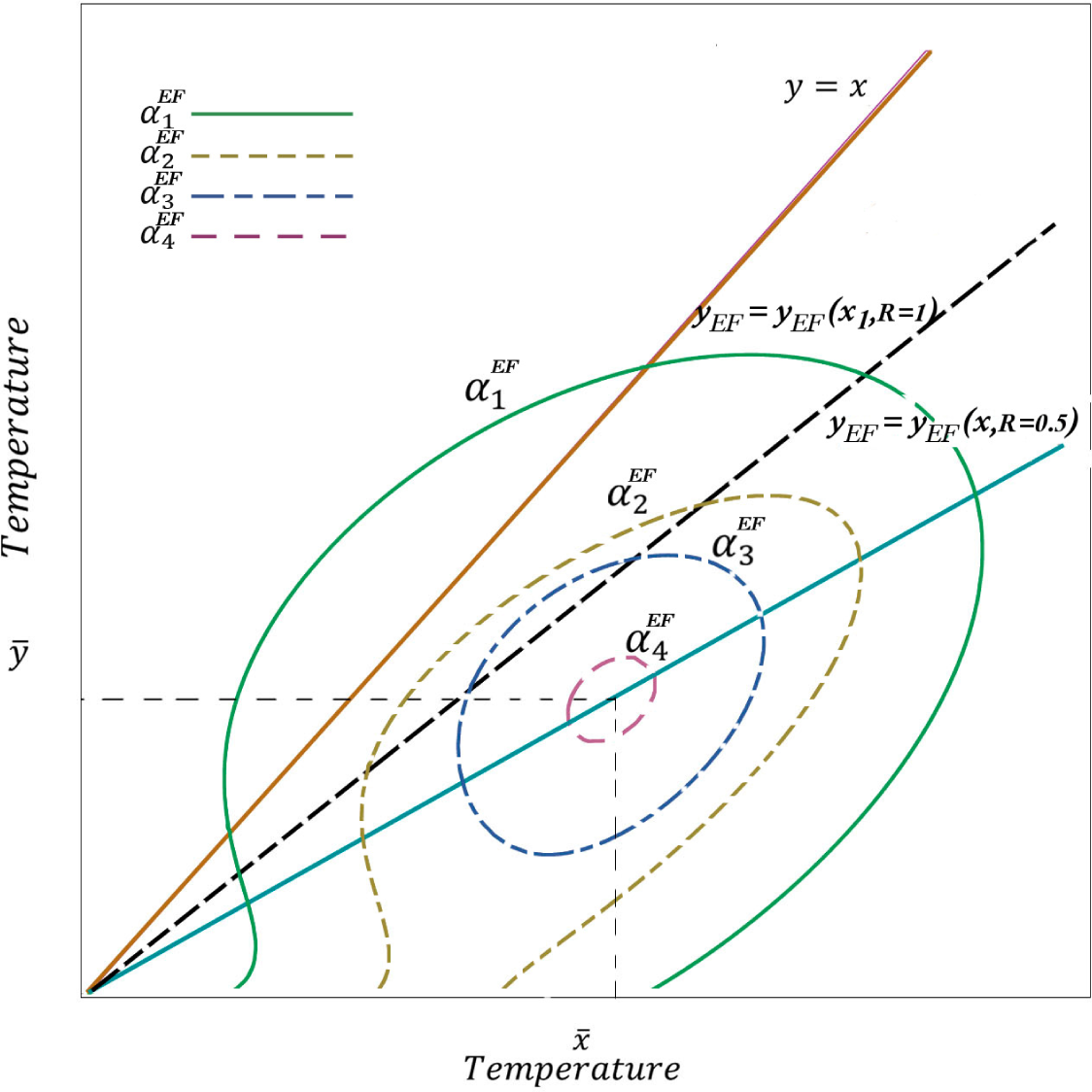
3.4. Maximum Ecological Function Regime

Following a similar procedure as in the previous section, the dynamic equations for x and y, but now at maximum EF conditions, are given by,
x ˙ E P = k C [ T 1 x + R 2 x 2 y ( 1 y R x ) ( R ( R x 2 + 8 y 2 ) R x R y 2 ) ( R x y ) ( R ( R x 2 + 8 y 2 ) R x + 2 y ) ] ,
and:
y ˙ E P = k C [ T 2 y R x y 2 ( 1 y R x ) ( R ( R x 2 + 8 y 2 ) R x R y 2 ) ( R x y ) ( R ( R x 2 + 8 y 2 ) R x + 2 y ) ] .
The Lyapunov function under maximum ecological function conditions is given as,
V ˙ E P ( x , y ) = k 2 C 2 { [ T 1 x + R 2 x 2 y ( 1 y R x ) Λ ( x , y , R ) ( R x y ) ( R ( R x 2 + 8 y 2 ) + 2 y R x ) ] 2 + [ T 2 y R x y 2 ( 1 y R x ) Λ ( x , y , R ) ( R x y ) ( R ( R x 2 + 8 y 2 ) + 2 y R x ) ] 2 } .
where Λ ( x , y , R ) = R ( R x 2 + 8 y 2 ) R ( x + 2 y ) R y. For this case, as occurred with Equation (30), it is easy to verify that V ˙ E F ( x , y ) = V E F x x ˙ + V E F y y ˙ = V E F , X ˙ 0.

4. Discussion

We have showed that the functions VEP(x, y) and VEF(x, y), given by Equations (29) and (33), which correspond to both maximum EP and EF conditions, respectively, are the Lyapunov functions for their corresponding dynamical system, that is, in both cases, the system is asymptotically stable [24]. To further explore the form of the functions VEP(x, y) and VEF(x, y), a set of curves are constructed to illustrate their behavior for the feasible region. Figures 2 and 3 show the level curves defined by VEP(x, y) = αEP and VEF(x, y) = αEF, respectively, for different values of the constant αEP and αEF. As expected, we observe in both cases that, as the constant value decreases, the surface also decreases towards the steady-state values ( x ¯ , y ¯ ), for the endoreversible and non-endoreversible cases, respectively.
Besides, in Figures 4 and 5, we show qualitative surface plots of VEP (x, y) and VEF (x, y). As we can see, for both cases, the surfaces resemble a basin, which indicates that the global stability of the system is preserved for different values of the irreversibility parameter R under both maximum EP and maximum EF conditions. Additionally, we performed numerical integrations of the system to further verify the global asymptotically properties for the regimes. In Figure 6, we present the results of numerical integrations of the system given by Equations (27) and (28) for the case of efficient power and Equations (31) and (32) for the case of ecological function. For illustrative purposes, we have considered four representative cases for the initial conditions (see the caption of Figure 6 for details). As we can see, in all cases, the internal temperatures evolve towards the steady state. For convenience, in this figure, we also include the case of MP previously reported in [20].
In order to compare the decaying rates of the internal temperatures, we also calculate the rate of change, d x d t and d y d t, for the evolution curves shown in the main frame of Figure 6. The results are depicted in the insets of Figure 6. We observe that for the Cases (1) and (2), the rate of change of x and y corresponding to the MP-regime are bigger than the ones corresponding to EF and EP, indicating that a fast approximation takes place under MP conditions, whereas for Cases (3) and (4), the opposite situation is observed. We recall that these results are valid for the particular values considered to perform the numerical integrations.
Moreover, we construct phase spaces for the cases R = 1, R = 0.8 and R = 0.6 to observe the trajectories’ approximation towards the steady state, that is to observe the way internal temperatures approximate their corresponding steady sate for each regime (Figure 7a–c). In all cases, the temperatures display a fast rate along the horizontal axes in comparison with the vertical approximation. Furthermore, from Figure 7a–c, it is noteworthy that the location of the steady state moves to the right and slightly downward as R decreases and also when the operation regime changes in the order MP, EP and EF. We notice that these approximations observed in the phase portrait are related to the existence of fast and slow eigendirections when a local stability analysis is performed around the steady-state values [17,20].

5. Concluding Remarks

The global stability of a CA-engine was analyzed by considering three regimes of performance: maximum power, efficient power and ecological function. The Lyapunov analysis presented here represents an attempt to characterize the global properties of the CA-engine model. Our results show that the stability is preserved for a range of parameter values, and the functions VEP (x, y) and VE(x, y) do not change its stability properties, even in the case when irreversibilities are present, that is for R < 1. Moreover, the findings of the global asymptotically-stable behavior of the equilibrium state were corroborated by means of numerical integrations performed over the dynamical equations of the system. The internal temperatures approximate the steady-state values, confirming that the system is stable for different initial configurations. Our results confirm the global stability properties of the CA-engine for three regimes of performance.

Acknowledgments

The authors thank F. Angulo Brown for fruitful comments and suggestions. We also thank EDI-IPN and COFAA-IPN and CONACyT, México for partial support.

Author Contributions

Marco A. Barranco-Jiménez and Lev Guzmán-Vargas designed the research; Israel Reyes-Ramírez, Marco A. Barranco-Jiménez and Adolfo Rojas-Pacheco performed the research and analyzed the data; Marco A. Barranco-Jiménez and Lev Guzmán-Vargas wrote the paper. All authors have read and approved the final manuscript.

Conflicts of Interest

The authors declare no conflict of interest

References

  1. Curzon, F.; Ahlborn, B. Efficiency of a Carnot engine at maximum power output. Am. J. Phys. 1975, 43, 22–24. [Google Scholar]
  2. Sieniutycs, S.; Salamon, P. Finite Time Thermodynamics and Themoeconomics; Taylor and Francis: London, UK, 1990. [Google Scholar]
  3. De Vos, A. Endorreversible Thermodynamics of Solar Energy Conversion; Oxford University Press: Oxford, UK, 1992. [Google Scholar]
  4. Wu, C.; Chen, L.; Chen, J. Recent Advances in Finite-Time Thermodynamics; Nova Science: New York, NY, USA, 1999. [Google Scholar]
  5. Chen, L.; Sun, F. Advances in Finite Time Thermodynamics: Analysis and Optimization; Nova Science: New York, NY, USA, 2004. [Google Scholar]
  6. Andresen, B. Current trends in finite-time thermodynamics. Angew. Chem. Int. Ed. 2011, 50, 2690–2704. [Google Scholar]
  7. De Vos, A. Efficiency of some heat engines at maximum-power conditions. Am. J. Phys. 1985, 53, 570–573. [Google Scholar]
  8. Yilmaz, T. A new performance criterion for heat engine: efficient power. J. Energy Inst. 2006, 79, 38–41. [Google Scholar]
  9. Arias-Hernández, L.A.; Barranco-Jiménez, M.A.; Angulo-Brown, F. Comparative analysis of two ecological types modes of performance for a simple energy converters. J. Energy Inst. 2009, 82, 223–227. [Google Scholar]
  10. Angulo-Brown, F. An ecological optimization criterion for finite-time heat engines. J. Appl. Phys. 1991, 69. [Google Scholar] [CrossRef]
  11. Velasco, S.; Roco, J.M.M.; Medina, A.; White, J.A.; Calvo-Hernández, A. Optimization of heat engines including the saving of natural resources and the reduction of thermal pollution. J. Phys. D 2000, 33, 355–359. [Google Scholar]
  12. Gordon, J.M.; Huleihil, M. On Optimizing maximum-power heat engines. J. Appl. Phys. 1991, 69. [Google Scholar] [CrossRef]
  13. Hoffmann, K.H.; Burzler, J.M.; Schubert, S. Endoreversible Thermodynamics. J. Non-Equilib. Thermodyn. 1997, 22, 311–355. [Google Scholar]
  14. Barranco-Jiménez, M.A.; Angulo-Brown, F. Thermo-economical optimization of an endoreversible power plant model. Rev. Mex. Fis. 2005, 51, 49–56. [Google Scholar]
  15. Arias-Hernández, L.A.; Ares de Parga, G.A.; Angulo-Brown, F. On Some Nonendoreversible engine models with Nonlinear heat transfer laws. Open Sys. Inf. Dyn. 2003, 10, 351–375. [Google Scholar]
  16. Santillán, M.; Maya-Aranda, G.; Angulo-Brown, F. Local stability analysis of an endoreversible Curzon–Ahlborn-Novikov engine working in a maximum-power like regime. J. Phys. D 2001, 34, 2068–2072. [Google Scholar]
  17. Guzmán-Vargas, L.; Reyes-Ramírez, I.; Sánchez-Salas, N. The effect of heat transfer laws and thermal conductances on the local stability of an endoreversible heat engine. J. Phys. D 2005, 38, 1282–1291. [Google Scholar]
  18. Páez-Hernández, R.T.; Angulo-Brown, F.; Santillán, M. Dynamic robustness and thermodynamic optimization in a non-endoreversible Curzon–Ahlborn engine. J. Non-Equilib. Thermodyn. 2006, 31, 173–188. [Google Scholar]
  19. Barranco-Jiménez, M.A.; Páez-Hernández, R.T.; Reyes-Ramírez, I.; Guzmán-Vargas, L. Local stability analysis of a thermo-economic model of a Chambadal-Novikov-Curzon–Ahlborn heat engine. Entropy 2011, 13, 1584–1594. [Google Scholar]
  20. Reyes-Ramírez, I.; Barranco-Jiménez, M.A.; Rojas-Pacheco, A.; Guzmán-Vargas, L. Global stability analysis of a Curzon–Ahlborn heat engine using the Lyapunov method. Physica A 2014, 399, 98–105. [Google Scholar]
  21. Chen, J. The maximum power output and maximum efficiency of an irreversible Carnot heat engine. J. Phys. D 1994, 27, 1144–1149. [Google Scholar]
  22. Ozcaynak, S.; Goktan, S.; Yavuz, H. Finite-time thermodynamics analysis of a radiative heat engine with internal irreversibility. J. Phys. D 1994, 27, 1139–1143. [Google Scholar]
  23. Barranco-Jiménez, M.A.; Sánchez-Salas, N.; Angulo-Brown, F. Finite-time themoeconomic optimization of a solar-driven heat engine model. Entropy 2011, 13, 171–183. [Google Scholar]
  24. Krasovskii, N.N. Stability of Motion; Stanford University Press: Stanford, CA, USA, 1963. [Google Scholar]
  25. Shampine, L.F.; Thompson, S. Solving DDEs in matlab. Appl. Numer. Math. 2001, 37, 441–458. [Google Scholar]
  26. Bogacki, P.; Shampine, L.F. A 3(2) pair of RungeâǍŞKutta, formulas. Appl. Math. Lett. 1989, 2, 321–325. [Google Scholar]
Figure 1. Schematic representation of a non-endoreversible Curzon–Ahlborn engine.
Entropy 16 05796f1
Figure 2. Qualitative plots of level curves of the Lyapunov function VEP(x, y) for the non-endoreversible case with R = 0.5. Here, the constant was chosen satisfying α 4 E P < α 3 E P < α 2 E P < α 1 E P. As a guide, we also show the lines yEP = yEP (x) and yEP = yEP (x, R), which represent the endoreversible (R = 1) and the non-endoreversible (R = 0.5) limits, respectively.
Entropy 16 05796f2
Figure 3. Qualitative plots of level curves of the Lyapunov function VEF (x, y) for the non-endoreversible case with R = 0.5. Here, the constant was chosen satisfying α 4 E F < α 3 E F < α 2 E F < α 1 E F. As a guide, we also show the lines yEF = yEF (x) and yEF = yEF (x, R), which represent the endoreversible (R = 1) and the non-endoreversible (R = 0.5) limits, respectively.
Entropy 16 05796f3
Figure 4. Qualitative surface plots of the Lyapunov function VEP (x, y), for different values of the irreversibility parameter R. We observe that in all cases, the surfaces are a basin shape-type, even when R takes small values (R < 1).
Entropy 16 05796f4
Figure 5. Qualitative surface plots of the Lyapunov function VE(x, y), for different values of the irreversibility parameter R. As in the case of VEP (x, y) (Figure 4), surfaces also are the basin shape-type.
Entropy 16 05796f5
Figure 6. (Main frame) Evolution of working temperatures vs. time t, for different initial conditions for the endoreversible case R = 1 (the cases R = 0.8 and R = 0.6 are not shown). We have considered four representative cases, where each has different initial conditions ( x 0 i , y 0 i ) (which will be useful for the description of Figure 7), with i = 1, 2, 3, 4. In all of the cases, both temperatures exhibit a decaying behavior towards their corresponding steady-state values, and we observe that x(t) approximates faster than y(t) for the four cases. To obtain the evolution as a function of time, the equations were numerically integrated using the Runge–Kutta triple (Bogacki et al. [25,26]). (Insets) First derivative with respect to time of the curves in the main frame. The rate of change reveals that fast approximations towards the steady state are observed for MP-conditions (Cases (1) and (2)), while the opposite situation is valid for Cases (3) and (4).
Entropy 16 05796f6
Figure 7. Qualitative phase portrait of x(t) vs. y(t) for the endoreversible case R = 1 (a) and the non-endoreversible cases R = 0.8 (b) and R = 0.6 (c) considering the three regimes of performance: MP, maximum EP and maximum EF conditions. In (a), the trajectories represent the four cases described in Figure 6. We use the same initial points to show the evolution towards the steady-state values. Notice that the steady-state coordinates move to the right and downward of their location for each regime and for the different values of R.
Entropy 16 05796f7

