Dynamical Non-Equilibrium Molecular Dynamics


Abstract
: In this review, we discuss the Dynamical approach to Non-Equilibrium Molecular Dynamics (D-NEMD), which extends stationary NEMD to time-dependent situations, be they responses or relaxations. Based on the original Onsager regression hypothesis, implemented in the nineteen-seventies by Ciccotti, Jacucci and MacDonald, the approach permits one to separate the problem of dynamical evolution from the problem of sampling the initial condition. D-NEMD provides the theoretical framework to compute time-dependent macroscopic dynamical behaviors by averaging on a large sample of non-equilibrium trajectories starting from an ensemble of initial conditions generated from a suitable (equilibrium or non-equilibrium) distribution at time zero. We also discuss how to generate a large class of initial distributions. The same approach applies also to the calculation of the rate constants of activated processes. The range of problems treatable by this method is illustrated by discussing applications to a few key hydrodynamic processes (the “classical” flow under shear, the formation of convective cells and the relaxation of an interface between two immiscible liquids).1. Introduction
The most widespread use of Molecular Dynamics (MD) [1,2], in the same spirit of Monte Carlo (MC) [3,4], is to compute the thermodynamic or statistical behavior of molecular systems at equilibrium. This means that, starting from the assumption of the validity of the ergodic hypothesis, dynamical (MD) or fictitious-time (MC) trajectories are used to sample the equilibrium distribution in phase space (MD) or in configurational space (MC). “Time” averages over the generated trajectories will thereafter provide the statistical properties of the system.
At variance with Monte Carlo, the dynamical approach of Molecular Dynamics can be directly extended to sample distributions corresponding to stationary non-equilibrium conditions, where there exists a stationary distribution but, at variance with equilibrium, its expression is not explicitly known. However, the statistical problem of sampling a time-dependent ensemble cannot be solved by generating states along a single dynamical non-equilibrium trajectory, as long as time cannot be taken as homogeneous and averages over time make no sense.
Generally, to compute macroscopic dynamical behaviors, as, e.g., in hydrodynamics, the assumption of time-scale separation is made and rigorous ensemble averages are substituted with short-time averages equivalent to local smoothing. This may not be the case, sometimes. Moreover, the statistical error implied by this procedure cannot be made as small as desirable and possible. These difficulties can be faced and solved.
In the nineteen-thirties, Lars Onsager [5] observed that an induced (non-equilibrium) relaxation towards equilibrium could be obtained by studying the regression of the corresponding spontaneous fluctuations at equilibrium. Later, in the nineteen-fifties, Kubo [6] provided a mathematical formulation of Onsager’s ideas by showing how the (linear) response of a system, initially at equilibrium, to a time-dependent (external) physical perturbation could be obtained by convoluting it with an appropriate equilibrium time-correlation function [7–9]. Kubo also derived the formal expression for the complete (linear and nonlinear) response.
In the case of Kubo’s procedure one does not need to make reference to an initial equilibrium state, but can, rather, refer to an arbitrary initial distribution at time t0 = 0 of the system. This result has an important consequence for Molecular Dynamics simulations, since it allows one to separate the problem of dynamical evolution from the problem of sampling the initial condition.
Starting from the mid-nineteen-seventies, the direct numerical simulation of the response was used in conjunction with a sample of initial conditions extracted from an equilibrium trajectory [10,11]. In this context, the problem of achieving a reasonable signal-to-noise ratio, even for weak perturbations, was solved for short times by introducing the so-called subtraction technique [12], which permitted one to verify, with surprising results [13], the range of the validity of linearity.
Some time later on, it was realized that the same approach could be used to calculate dynamical properties for rare events (e.g., transmission coefficients) by averaging the dynamical response over time-dependent trajectories started from initial conditions sampled from a constrained/conditional equilibrium ensemble [14–18].
Quite recently, finally, the idea of creating a large sample of non-equilibrium trajectories starting from a given initial distribution has been extended to cover whatever distribution that can be sampled starting from an equilibrium or a non-equilibrium, but stationary, dynamics. In particular stationary non-equilibrium ensembles can be generated by suitably restraining standard MD simulations.
In particular, we will illustrate the approach by reporting the results of a study of the time evolution of classical fields, including the onset of convective cells and the relaxation of hydrodynamic interfaces in simple liquids. In this context, we will also briefly address a conceptual difficulty of the approach, due to the possible existence of more than one macroscopic state associated with specific perturbations. In particular cases the problem can be circumvented.
The structure of the paper is as follows. In Section 2 we derive the general framework and specify the possible forms for the initial ensemble. In Section 3 we present a few successful applications of the method. Finally, in Section 4 we try to assess the situation and sketch an outlook.
2. Dynamical Approach to Non-Equilibrium: Theoretical Background
2.1. General Formulation
We start considering, in a very general way, a (classical) dynamical system with n degrees of freedom, whose time evolution is described by a set of first order differential equations in a phase space of dimension 2n. We will refer to the phase space variables in a collective way with the vector formalism Γ⃗ = {q1, p1, q2, p2,...,qn, pn}, where the q’s and the p’s reduce to the usual coordinate-momentum pairs for Hamiltonian dynamics. The equations of motion can be written in the compact form
Time evolution in phase space can be alternatively expressed in term of the Jacobian J (Γ⃗(t), Γ⃗(t0)) of the time transformation from Γ⃗(t0) to Γ⃗(t). The phase space element d2nΓ(t0) at time t0 transforms into the volume element d2nΓ(t) = J (Γ⃗(t), Γ⃗(t0)) d2nΓ(t0) at time t, where J = det J obeys the differential equation [23]
The solution of Equation (12) can be retrieved along the same lines followed for Equation (2) and the results can be formally written in closed “operatorial” form
The average over the (non-)equilibrium ensemble of a physical observable O(t) = 〈Ô(Γ⃗)〉t or, more generally, of a macroscopic field O(x⃗, t) = 〈Ô(x⃗, Γ⃗)〉t = 〈∑jÔ(Γ⃗)δ(x⃗ − R⃗j)〉t (the sum is over the particles) can be defined as
We can make the time evolution explicit by means of the adjoint time evolution operator ρ(Γ⃗; t) = Ŝ†(t, t0)ρ(Γ⃗; t0) and then, by taking advantage of the fact that Ŝ† is the adjoint of the dynamics, we can transfer the effect of time evolution to the physical observables
Despite the apparent complexity of the time evolution operator Ŝ(t, t0) in Equation (5), its action is a task that can be simply accomplished by MD, i.e., by the numerical integration of the evolution defined by Equation (1). Note that all this is possible thanks to the fact that the Liouville equation can be integrated by the method of characteristics.
In the following, we will deal with fluid systems where the relevant macroscopic fields are [24] the density field ϱ(x⃗, t), the velocity field v⃗(x⃗, t) and the temperature field T(x⃗, t):
2.2. Ensembles at t0
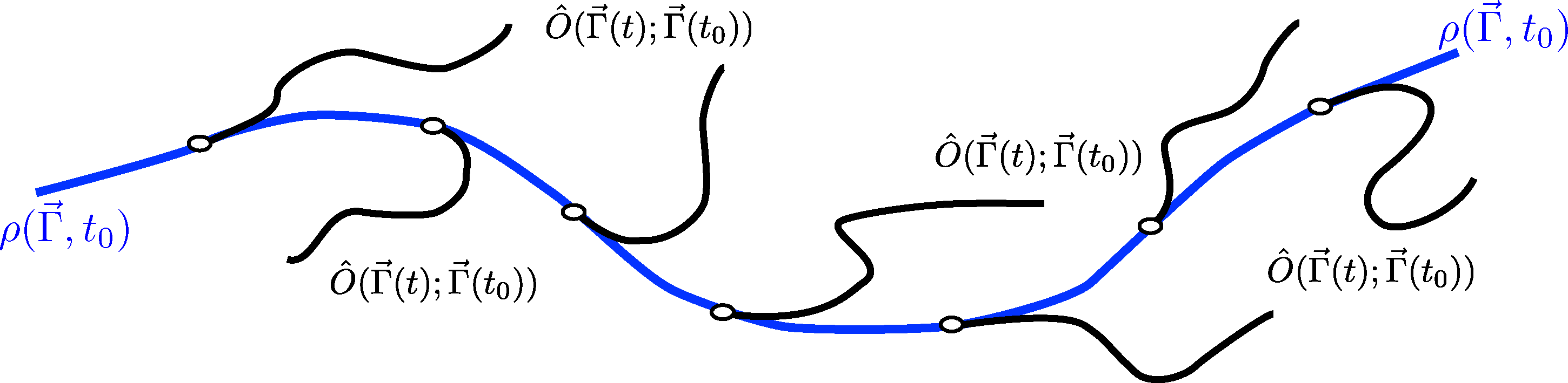
Equations (17) and (18) express what we like to call the Onsager–Kubo relations and state that we can obtain the time evolution of a macroscopic observable or of a macroscopic field as the average of the time evolved corresponding microscopic expression over the initial-time-ensemble described by the phase space density ρ0 = ρ(Γ⃗; t0).
If the ensemble at the initial time t0 can be simulated by a dynamical system in stationary conditions, then such a probability density function can be sampled by MD, generating a set of (possibly independent) phase space points distributed according to ρ0. From each of these points, one can then start an independent dynamical trajectory along which the observables Ô(Γ⃗; t) and Ô(x⃗, Γ⃗; t) can be computed. Finally, by averaging over all the trajectories, the values of the involved observables at time t, one can obtain the macroscopic time-dependent behavior of the system as visualized in Figure 1.
In order to use MD to sample the appropriate initial ensemble at time t0, one needs to define, for any specific problem, the dynamical evolution, Equation (1), and the auxiliary conditions to which the systems is subjected. Sometimes, but not always, this will be possible within the Hamiltonian formulation of the dynamics.
3. D-NEMD Selected Applications
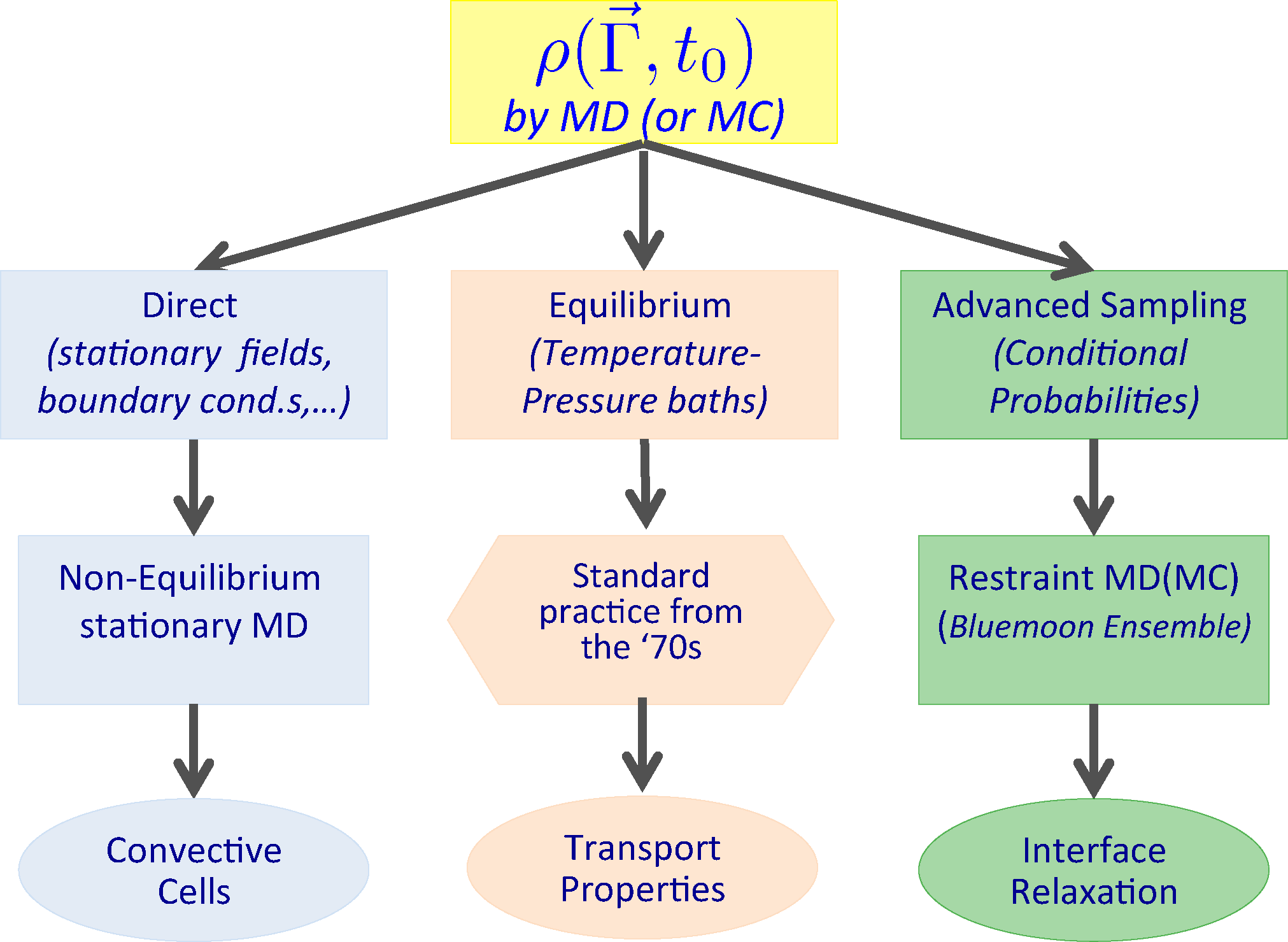
We will now list a number of cases, which will later be illustrated with the corresponding application. Transport properties, like viscosity, thermal conductivity, etc., have been computed and their linearity range investigated by non-equilibrium MD since the 1970s [10–12,25–34]. These results were obtained by measuring on a computer the mechanical response when switching on the external (at the beginning Hamiltonian and later on, more generally, also non-Hamiltonian) perturbation applied to a model system initially at equilibrium. In other words, we identify in the present case the ensemble at time t0 with the statistical mechanics equilibrium ensemble, while the dynamical trajectories are carried out under the influence of an external (time-dependent) force field.
More generally, we can generate (and sample) initial ensembles by less trivial procedures, e.g., in the case of the formation of convective cells, gravity is considered as the external perturbation to be applied on a system initially in a steady state under the effect of a thermal gradient. The ensemble at time t0 no longer corresponds to the equilibrium one, but it is set up by introducing a stationary boundary perturbation which, in the specific case, is just an ad hoc boundary condition, which models a thermal wall stochastically. Moreover, a confining wall, present in the form of an external field acting at the boundary on each particle, confines the system in the simulation box. This boundary condition is perfectly compatible with the presence of a gravity field.
Another possible case we will consider is the relaxation to equilibrium of an interface between two immiscible liquids, starting from an imposed, non-equilibrium, condition in which the curvature of the interface is maintained by a macroscopic restraint fixing the shape of the initial interface. The ensemble at time t0 is described by a conditional probability density in which an ad hoc restraint is imposed on a field-like observable. The sample is generated by using an advanced MD sampling technique, where the dynamical trajectory evolves under the effect of a suitable restraining potential, from which we can extract an unbiased sample of the conditional probability density function. Time-dependent averages are then taken over dynamical trajectories generated according to the un-restrained dynamics of the systems. The different situations described are summarized in Figure 2.
3.1. Transport and Linear Response
Linear Response Theory is a nice result of the nineteen-fifties in the theory of irreversible processes [6], where well-defined microscopic expressions for all transport coefficients have been derived in terms of a properly chosen perturbation [7,8,35,36]. In the Dynamical approach to Non-Equilibrium Molecular Dynamics (D-NEMD) framework it has been possible to investigate the linear and, more generally, the non-linear response by making reference to the canonical ensemble for sampling the initial conditions at time t0.
3.1.1. Hamiltonian Perturbations
For a system of particles in three dimensions described by the usual set of Cartesian coordinates and momenta, {R⃗j, P⃗j, j = 1, 2,... }, the perturbation can be put in Hamiltonian form by choosing a physical property Â(x⃗|Γ⃗) = ∑j Aj(Γ⃗)δ(x⃗ − R⃗j) that describes the coupling of the system to the applied external local field ψ(x⃗, t) = φ(x⃗)χ(t), whose time-dependent intensity χ(t) can be constant or periodic or even arbitrary, generating corresponding flux conditions. Especially important are the cases in which the perturbation is either a step function θ(t − t0) (θ(t > t0) = 1, θ(t < t0) = 0) or a Dirac delta impulse δ(t − t0), at t = t0, after which the system is left free to relax. In the linear regime, the general response can be computed as the superposition of these impulsive responses. One then derives the equations of motion using the standard Hamiltonian route, where we start by separating in the Hamiltonian (Γ⃗, t) = 0(Γ⃗) + p(Γ⃗, t) the time-dependent perturbation term
The structure of the equations of motion can be broken into the two terms of the Liouville operator defined in Equation (2), ι̂(Γ⃗; t) = ι̂0(Γ⃗) + ι̂p(Γ⃗; t), with the partial Liouville operator ι̂0 defining the dynamical evolution in phase space for the sampling of the ensemble at time t0. Accordingly, the corresponding evolution operator for the stationary dynamics will be called Ŝ0(t). The dynamics of the time-dependent trajectories will be generated by the t0-(time dependent) evolution operator Ŝ(t, t0), obeying the (usual) Dyson equation
3.1.2. Non-Hamiltonian Perturbations
A more general scheme has also been used for bulk perturbations, where the new equations of motion, which cannot be derived from a time-dependent Hamiltonian in a way that remains consistent with applied (periodic) boundary conditions, are obtained from Equation (23) by substituting the terms derived from the Hamiltonian perturbation hp, with two sets of “ad hoc” phase space functions {C⃗j(Γ⃗), D⃗j(Γ⃗), j = 1, 2,...}:
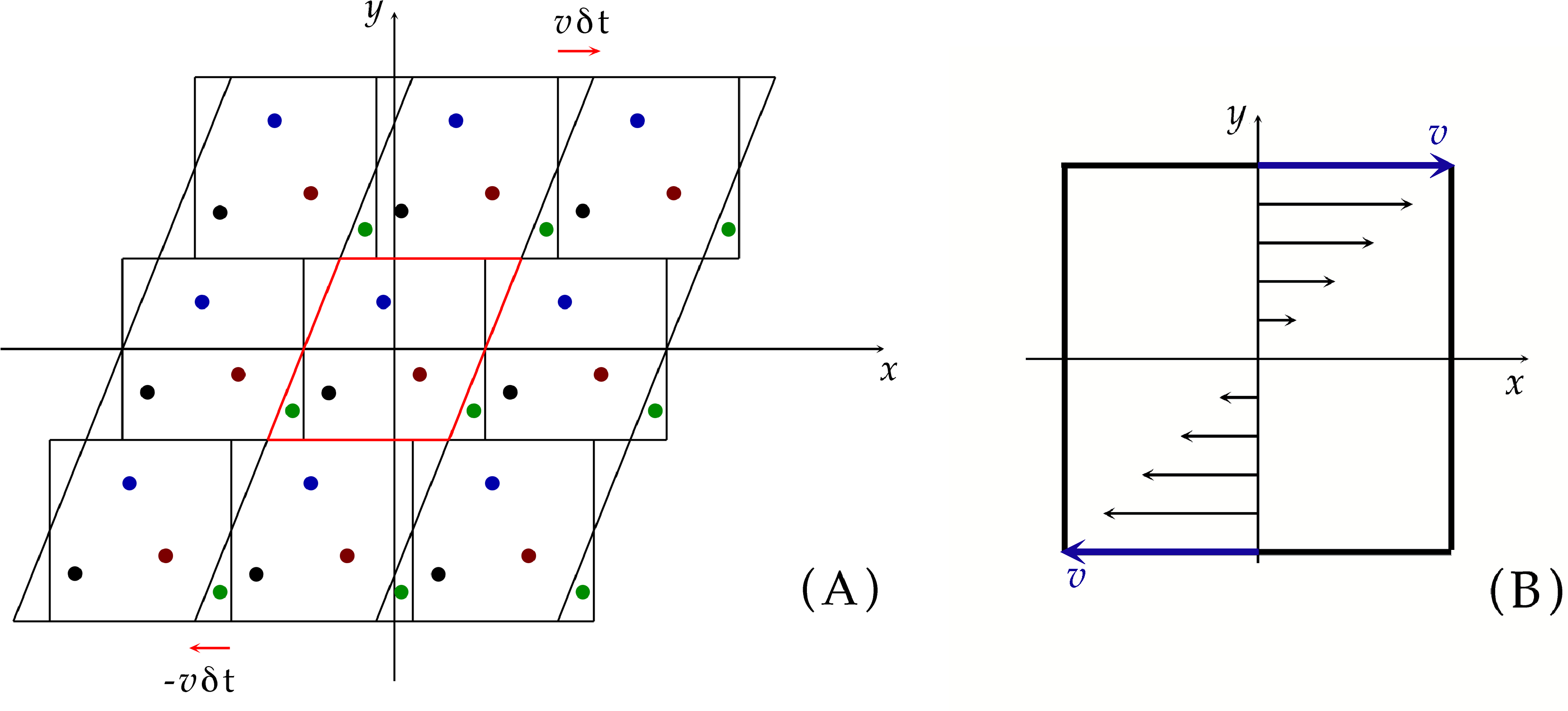
In the typical setup for a planar Couette flow, one establishes a gradient of the x-component of the velocity along the y-axis of the simulation and measures the response using as an observable the xy component of the pressure tensor σxy, which can be written, for a system where the potential U is given by a sum of pair interactions, as
For the purpose of illustrating the method in the original applications, when the ensemble at the initial time t0 is an equilibrium ensemble, we will restrict ourselves to the simple case of shear (Couette) flow. We would like to mention, however, that also elongational flows [41,43–46] and, later on, mixed shear-elongational flows [47–49] have been simulated both in atomic and molecular fluids. In these cases, it becomes technically much more difficult to maintain for an indefinite length of time the periodic boundary conditions and, for that, we refer the interested reader to [50,51].
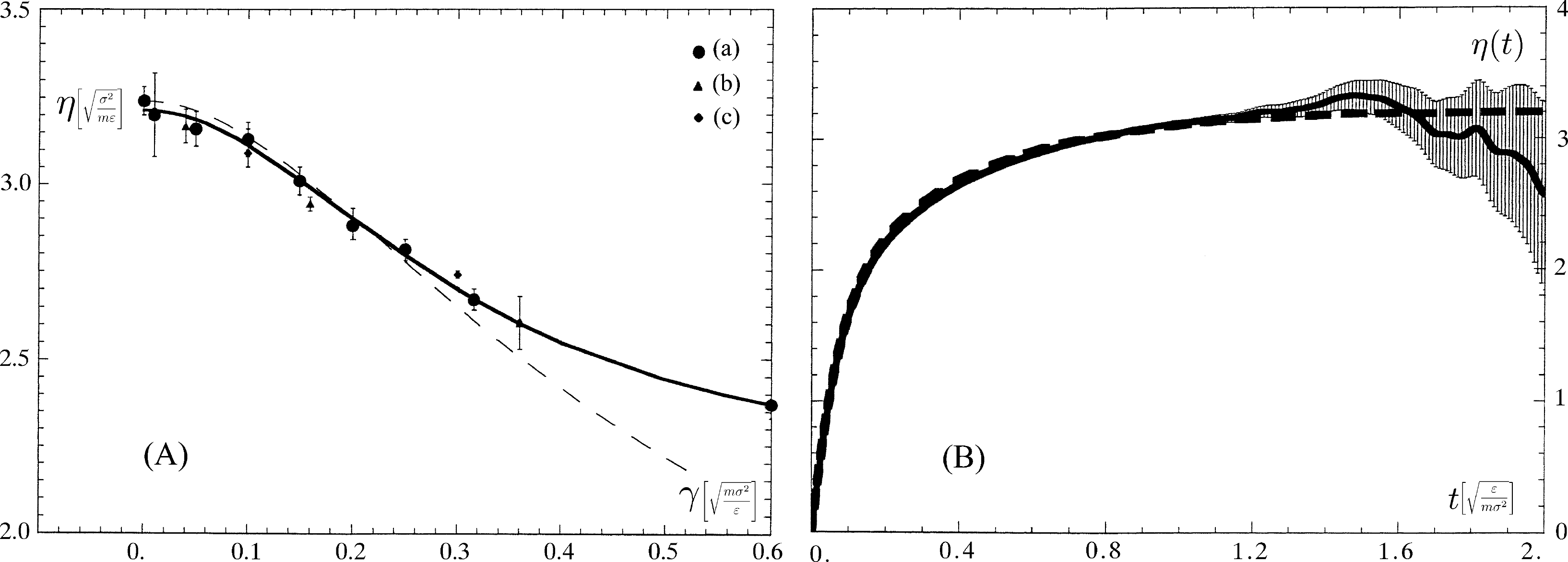
In Panel (A) of Figure 4, we show the results of a calculation [52] with a step function perturbation on a Lennard–Jones (LJ) fluid at the triple point, ϱ = 0.8442 and kBTp = 0.725 in reduced LJ units, i.e., ε for energy, σ for distances and the particle mass m for masses. The temperature of a system of 2,048 particles was controlled using a Nosé–Hoover thermostat [22], both on the long equilibrium trajectory, which samples the (independent) initial conditions from a canonical ensemble at temperature Tp and on the non-equilibrium trajectories to handle the heat produced, especially at high shear rates. The behavior of the time-dependent viscous response for the case of a t0 = 0 impulsive perturbation with a δ(t − t0) term was used to investigate the range of validity of the Linear Response Theory for very small shear rates by comparison with the running time integral of the corresponding stress autocorrelation at equilibrium [53].
3.2. Non-Equilibrium (Steady State) Initial Conditions at Time t0
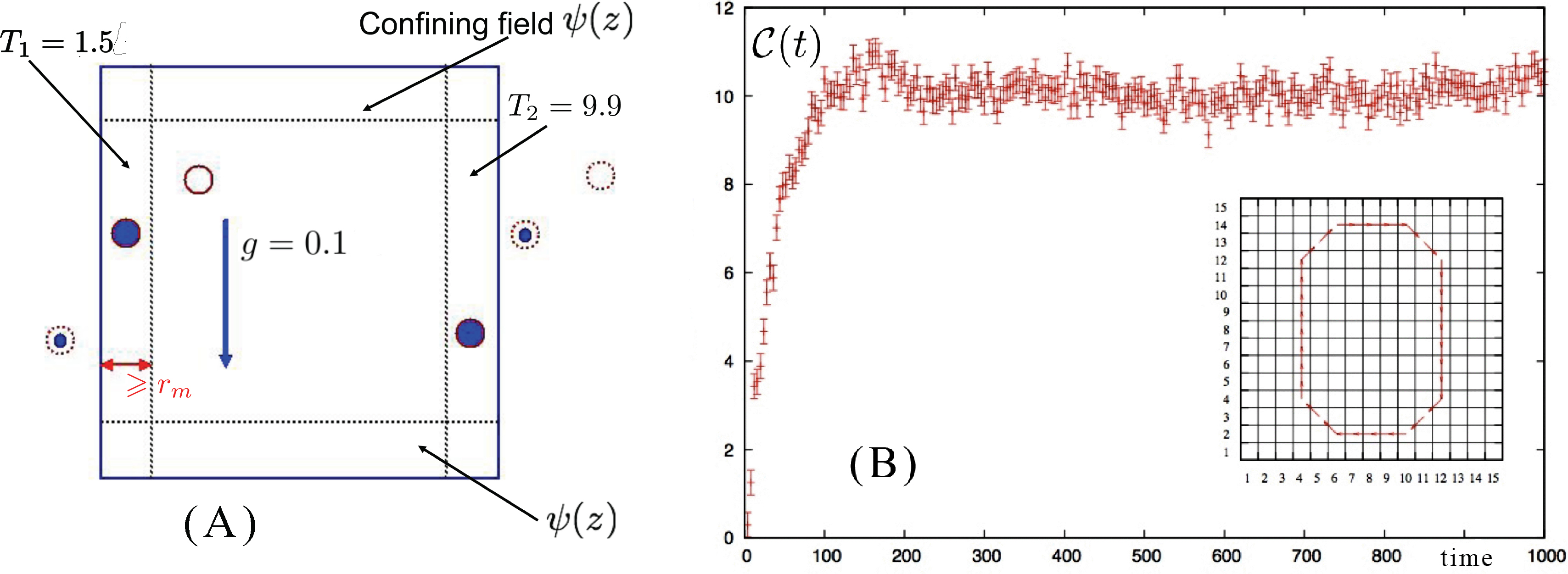
The D-NEMD approach can be used also to follow the transient evolution of a system, which, starting from an out-of-equilibrium state under the effect of a stationary thermodynamic field, reaches a final (different) non-equilibrium state in response to an additional external perturbation. Below, we illustrate the approach with a case worked out in [57]. This is the case of the build up of a convective roll in a two-dimensional (2D) model fluid kept in an out-of-equilibrium condition by the presence of a thermal gradient when an external gravity field is (instantaneously) switched on.
The 2D system is composed of N = 5, 401 identical particles in a square box of size L in the xz plane with periodic boundary conditions along the x direction and a pair of confining walls along z obtained by means of an external field ψ(z), acting at the top and the bottom of the simulation box to avoid the drifting away of the particles, which interact with each other via a purely repulsive (2D) Weeks–Chandler–Andersen (WCA) [58] pair potential obtained by truncating the Lennard–Jones potential at its minimum rm = 21/6σ and shifting its value by ε in such a way that both the force and potential are continuous and equal to zero for r ⩾ rm.
We have seen how D-NEMD can be used to illustrate the build up of a convective roll when a gravity field is instantaneously switched on in a system where a stationary (non-equilibrium) thermal gradient was already present. This is not the only case in which a convective roll can be observed. Indeed, keeping the same geometry for the system, i.e., with the gravity field orthogonal to the thermal gradient (Panel A of Figure 5), one could alternatively start from initial conditions in which the system is at equilibrium in the presence of the gravity field and, then, follow the dynamics when the thermal gradient is instantaneously switched on or even start from a homogeneous fluid at equilibrium and instantaneously switch on both the gravity field and the thermal gradient [57]. In all these cases, although following different paths, the system eventually reaches the same (macroscopic) final steady state with the formation of a clockwise rotating convective roll, centered at the center of the box.
Complications arise if the system is setup with a different geometry, e.g., in the case of Rayleigh–Bénard convection when the direction of the thermal gradient is parallel to the direction of the gravity field. The system has a higher symmetry and rolls rotating both in the counterclockwise and clockwise directions are possible. This implies that the D-NEMD averages cannot be carried out directly, as in the case we have described so far. In fact, now, in the ensemble of individual trajectories, one samples with equal probability the initial conditions leading to clockwise or to counterclockwise rolls. Performing ensemble averages without paying attention to the direction of rotation would give a wrong result. One needs either to enforce a mechanism that breaks this symmetry or to weight trajectories differently, according to the direction of rotation of the convective roll. The latter was the choice applied in [57], where it was simply impossible to fix a priori, by tweaking the initial conditions, the final rotation direction of each trajectory. Instead, the direction of the convective roll rotation was analyzed in the steady-state part of each trajectory by time averaging the velocity field over the last 10,000 steps. The ensemble averages were consistently computed, afterwards, by taking the specular image of the fields when the roll rotation was opposite to the one (arbitrarily) chosen as the reference.
3.3. Sampling from Conditional Distributions at Time t0
Probably the most interesting application of the D-NEMD procedure is when the non-equilibrium dynamical trajectories start from states corresponding to a very unlikely fluctuation and we want to follow dynamically the way in which the system relaxes back to equilibrium. An efficient sampling of the points in phase space representing the initial condition cannot be achieved just by waiting long enough for the desired event to occur during a standard MD trajectory, but more advanced methods are required to enhance the sampling. Whenever the conditions can be described using an “order parameter”, i.e., an appropriate phase space function or field, one can define a macroscopic constraint that applied to the system will allow one to explore the interesting, but unlikely, region of phase space. A viable method in many cases is the well-known Blue Moon approach [15,59], where the conditional probability density is constructed by augmenting the dynamical system with a set of holonomic constraints that force the system to explore states on the specific hypersurface of interest in phase space. The points sampled on a dynamical trajectory subject to constraints, however, cannot be directly used to start the time-dependent non-equilibrium trajectories, because of the unphysical additional conditions enforced on velocities to keep the dynamics on the constrained hypersurface. In the Blue Moon approach, such caveats are overcome, the correct procedure is outlined in [15], requiring, first, an apt resampling of the velocities and, then, an appropriate reweighting when computing the time-dependent averages. The Blue Moon approach was initially devised and successfully applied to the calculation of rate constants for activated processes. In particular, the rate constants are defined in terms of the product of two terms: a transition state theory term and a “transmission coefficient” (i.e., the plateau value, in the intermediate time scale, reached following the transient behavior of the time-dependent values of the reaction coordinate(s) [14,60]). The calculation of the transmission coefficient is a task that can be accomplished exactly along the same lines of the proposed D-NEMD approach.
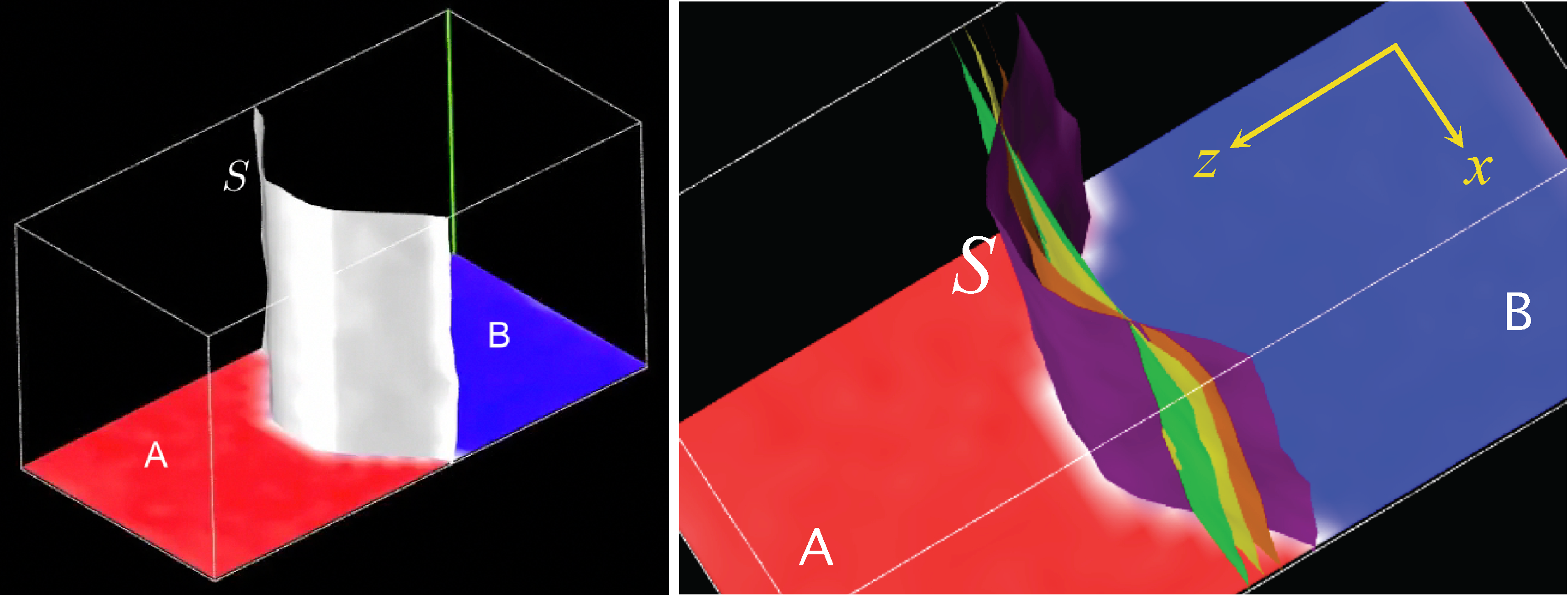
As a more advanced illustration of D-NEMD when sampling from a conditional probability density, we describe the case of the hydrodynamic relaxation to equilibrium of the interface between two immiscible liquids [61]. The relaxation can be described by following the time evolution of the difference of the density fields of the two species A and B, Δϱ(x⃗; t) = ϱA(x⃗; t) − ϱB(x⃗; t), and the associated velocity field ϱv(x⃗; t). The distribution at time t0 corresponds to the stationary conditions of the system subject to a macroscopic restraint that forces a non-equilibrium geometry for the interface. This requires the implementation of a method, like the Blue Moon one, that allows one to sample the conditional probability density associated with the constraint. However, using the Blue Moon approach for vector or field-like constraints can become considerably cumbersome and rather inconvenient in practice, especially for molecular systems where constraints are already used in the force field to impose molecular geometries. A much more practical alternative is to use restrained MD, where one substitutes the constraint with an equivalent restraining potential in terms of an additional coupling parameter, asymptotically reproducing unbiased constrained conditions. Let us summarize the restraint MD approach for the case in which the constraint is imposed on a field-like observable, as for the density difference Δϱ (x⃗, t). Constraining the shape of the interface S corresponds to specifying the set of spatial points {x⃗S} where Δϱ (x⃗S, t) = 0.
According to Irving and Kirkwood [24], we associate with this macroscopic field a microscopic observable
Consider, now, a system described by the Hamiltonian
The idea of using a biasing potential to sample unlikely points in configuration space was pioneered by Torrie and Valleau for MC simulation [62], then presented in this form in [63]. However, while in their case of umbrella/window sampling, the bias is tuned in such a way to sample, in a statistically significant manner, a wider portion of the configuration space, in the restraint MD approach, one considers high enough values of the tunable parameter k with the aim of sampling the conditional probability associated with the portion of phase space representing a rare region of interest. Indeed, using that , one recovers, in the limit βk → ∞, the joint probability density
The choice of a restraining potential, which depends only on the coordinates of the particles, as in this case, does not influence the probability density in the momentum space, which remains the Maxwellian (equilibrium) distribution and, at variance with the Blue Moon approach, independent points along the stationary restrained MD trajectory can be directly taken as initial configurations representative of the probability density at time t0. Moreover, if needed, the restrained MD approach can be further generalized to enforce a more general macroscopic constraint affecting also the momenta of the particles, for example, coupling it with the ad hoc boundary conditions and the localized velocity sampling described in Section 3.2 to impose a non-uniform macroscopic velocity field or a temperature gradient in the system.
The definition of the microscopic field in Equation (31) has still one important drawback, which can prompt major issues in particular conditions. In fact, because of the presence of δ-functions in the definition, as a particle crosses the border between one cell and the neighboring one, the integrals that define the macroscopic field at the two corresponding points in space change by, plus or minus, respectively, a finite value introducing discontinuities in the restraining potential in Equation (32). This results in the (highly undesirable) appearance of impulsive terms in the forces on the atoms. Consider the δ(x⃗ − R⃗j) function contribution to the integral in Equation (31) for a specific particle j. This is given by the products of three terms, corresponding to the orthogonal directions in space, where each of them is the difference of the values of the cumulative distribution at the edges of the α − th cell. The cumulative distribution for the delta function δ(ξ) is the step function θ(ξ), {θ(ξ < 0) = 0, θ(ξ > 0) = 1}, so that each of the above three terms can only be either zero or one. In order to smooth the restraining potential, we need to replace the step function with a smoother function, like a sigmoid, resulting in a continuous variation, between zero and one, of each term in the product. This is equivalent to giving a finite extension to the particle size, resulting in the possibility that a particle contributes, fractionally, to the density field of more than one cell at the same time. In this way, the restraining potential changes smoothly with the motion of the particles in time, without discontinuities when particles cross the cell borders. One possible choice for such function is given by the error function, which corresponds to replacing the delta function by the equivalent Gaussian, in the limit a → 0, where the parameter a gives the order of magnitude for the (1D) size of the particle. Within such an approximation, Equation (31) becomes
The two fluids, A and B, are modeled using identical Lennard–Jones particles with mass m and (unique) parameters σ = σAA = σBB = σAB and ε = εAA = εBB = εAB for the LJ potential. The immiscibility is obtained by removing the attractive term for the pair interactions between a particle of type A and a particle of type B, keeping only the purely repulsive part, i.e., taking u(r = |R⃗A − R⃗B|) = 4ε [σ/r]12. The simulation was performed at a fixed temperature kBT = 1.5ε on a system totaling 171,500 particles, of which 88,889 for Fluid A and 82,611 for Fluid B, in a rectangular parallelepiped box with the same width and height w = h ≈ 44 and double length d ≈ 88, corresponding to an average particle density n = 1.024, where all figures are in reduced LJ units. The density and temperature are in the fluid region of the phase space of a pure LJ fluid. In order to follow the behavior of the density and velocity fields, the space was discretized using 5,488 cubic cells arranged on a 14 × 14 × 28 grid. In this way, local field values are obtained averaging out on roughly 30 particles in each cell. For the ensemble at time t0, the initial configuration for the interface between Fluid A and Fluid B is defined by selecting the m cells (centered on the mesh points, x⃗α, α = 1, 2,...,m), which are cut across by the ideal cylindrical surface, S̃,
A long, 106 MD restrained trajectory was then carried out, with that same time step, taking out, at regular intervals of 25,000 steps, the configuration of the system in phase space. A set of 40 independent initial conditions was collected in this way, and from each of them was started, now with a regular time step δt = 4.56 · 10−3, a 25,000-steps unrestrained MD trajectory at constant energy, i.e., using the equations of motion derived only from the Hamiltonian (Γ⃗), given in Equation (32). The D-NEMD averaging procedure was used with those 40 trajectories to compute the time-dependent behavior of the macroscopic density and velocity fields, discretized on the previously mentioned cubic mesh.
In the right panel of Figure 7, the dynamical behavior of the interface is shown by plotting the isosurfaces Δϱ(x⃗) = 0 for four successive times.
One can see that the interface curvature diminishes progressively towards the flat, equilibrium condition, while maintaining (approximatively) both the initial uniformity along the direction of the y-axis and the initial mirror symmetry with respect to the middle yz-plane. Small deviations are present, as expected, considering that this macroscopic field results from averaging over a relatively small sample of 40 independent trajectories. They are compatible with the expected amplitudes of the equilibrium fluctuations of the interface. Relaxation of the initially curved surface reaches the flat equilibrium condition fully in a time lapse of approximatively 20,000 steps, i.e., something just short of 100 LJ time units. One can use this information to estimate the order of the relaxation time and, from it, a maximum value vmax ≈ 0.5 in LJ units for the average velocity field at the mid-point along x of the interface, i.e., in the region corresponding to the maximum displacement at time t0 of the interface. If one takes the LJ parameters of argon (for which σ = 3.405 · 10−10 m and the unit of time corresponds to τ = 2.156 · 10−12 s), this value translates to an experimentally convincing velocity of ≈ 80 m · s−1.
The second interface on the sides of the MD box remains flat, with even smaller deviations, all along the 25,000 time steps. There seem to be no significant effects on it as a result of the relaxation process, which takes place in the middle of the box. The reason for this will become evident after looking at the time-dependent behavior of the velocity field. We have shown, in fact, how the D-NEMD approach provides very detailed information on the hydrodynamic behavior of the system and unravels the underlying physical mechanisms.
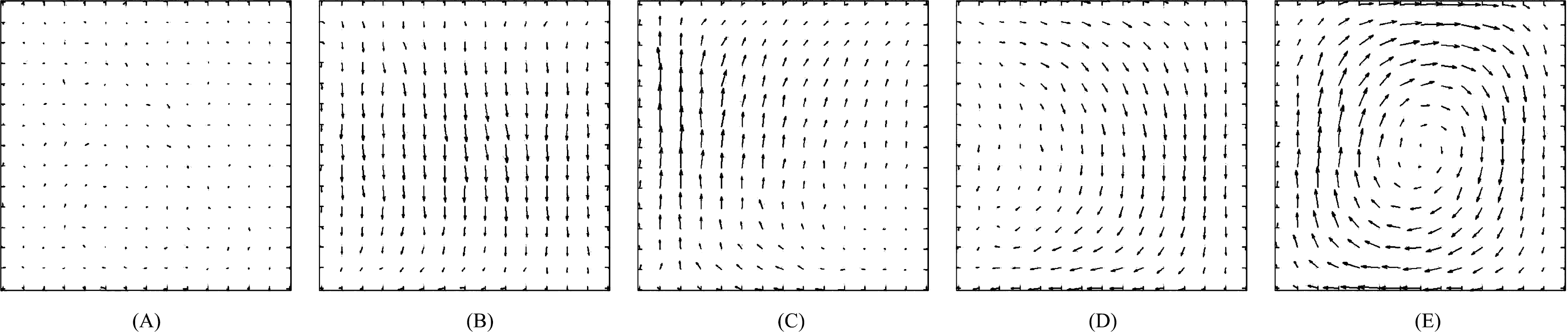
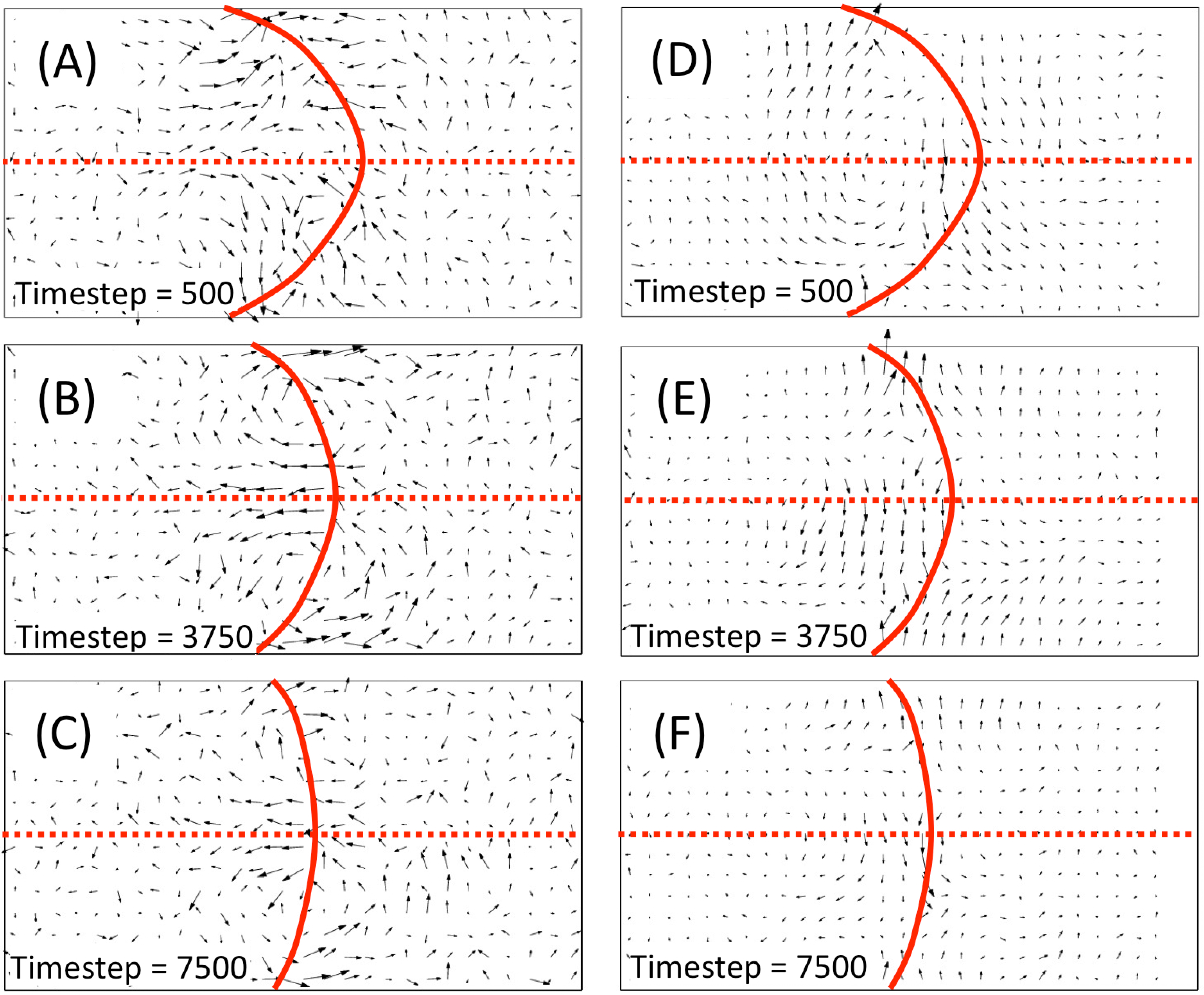
Starting from Equation (20), the discretized velocity field is calculated accordingly to:
Snapshots at three successive times are shown. In the snapshot taken 500 time steps after t0, one can notice the build up of some coherence in the velocity field, which becomes structured in a region that is, along the z-direction, about twice the size of the width of the curved interface, the projection of which is represented by the contour line at the value Δϱ = 0. For the sake of clarity, the symmetry yz plane is as well highlighted by a dashed straight line. One can distinguish a quasi-symmetric two-tail profile, where the push towards the edges of the interface appears to be more pronounced than the one, in the opposite direction, in the region near the center of the interface (Panel A). This behavior marks the initial build up of a more stable two-roll velocity profile, of roughly the same width across the interface region in the A and B fluids, which becomes very evident after 3,750 steps (Panel B) and is still neatly visible and qualitatively unchanged, even after 7,500 steps from t0, when the curvature of the interface is significantly reduced (Panel C).
One can notice that the size and the intensity of the field has decreased, but the profile remains highly symmetrical along the mirror symmetry plane. All along, one can notice also that the field in the extreme sides of the simulation box remains essentially unperturbed, which explains why the second flat interface at the boundary is not affected in any significant way and remains stable during the whole relaxation process of the curved interface. It is very interesting to compare these insights on the hydrodynamic processes underlying the interface relaxation, as given by the time-dependent behavior of the dynamical response calculated using the D-NEMD procedure, with the standard approach used on single trajectory simulations of hydrodynamic processes. Starting from the local equilibrium hypothesis of hydrodynamic theory, based on the assumption of a time scale separation between the fast microscopic motion of the particles and the slower hydrodynamic processes, the macroscopic fields are computed as local time averages on the short time scale τ of the atomistic processes [64].
By applying this approach to the time evolution from a single initial condition, one obtains the results shown in the right panels of Figure 8. At first glance, the velocity field appears to be much smoother than the D-NEMD result, which is relatively noisy due to the limited size (40) of the sample of initial conditions used. However, the picture that is returned is quite different, with the physical mechanism exposed by the D-NEMD procedure effectively washed out by the local time averaging, which also presents a velocity field that does seem to violate the mirror plane symmetry initially imposed on the system at time t0, contrary to the more convincing evidence, given from the D-NEMD results, of a relaxation mechanism satisfying, on average, such symmetry at all times along the dynamical trajectory.
4. Conclusions and Perspectives
In this paper, we have presented a dynamical approach to non-equilibrium MD, which makes it possible to compute, numerically, but, otherwise, rigorously, time-dependent non-equilibrium responses, i.e., to observe directly transient responses in non-stationary regimes. We have shown that using a proper simulation setup, it is possible to go beyond the usual situation of initial equilibrium conditions to treat interesting cases in which the initial condition is either a stationary non-equilibrium or a constrained equilibrium condition dictated by means of a macroscopic constraint, which can be expressed, in a general way, either as a scalar or field-like observable, outlining also the connections of the D-NEMD approach to the Blue Moon method [15] to compute the transmission coefficient contribution to the rate constants of activated processes.
We illustrated a few applications of the method starting from the early, historical, approach to the calculation of transport properties in the lines of Linear Response Theory and beyond, to a couple of recent atomistic simulations of hydrodynamic processes: the establishing of a convective cell, when gravity is switched on in the presence of a stationary thermal gradient, and the relaxation of an initially curved interface between two immiscible liquids. We have shown that the method generates rigorous time-dependent non-equilibrium averages, providing valuable insights on the mechanisms of hydrodynamic processes that can be missed using a method like the local time average, which cannot have a rigorous justification, presents a statistical error that cannot be reduced at will and, finally, as we have seen above, can bias the statistical response. A word of caution is needed, though. The time-dependent ensemble averages are meaningful only if the thermodynamical response is unique [65]. Whenever this is not the case, the meaning of the statistical averages becomes questionable. To our knowledge, in these cases a systematic answer does not exist for the non-equilibrium thermodynamic response and problems have to be treated on a one-by-one basis.
In summary, with the outlined exceptions, D-NEMD is a method ready for challenging applications, by which it is possible to study complex time-dependent phenomena using only the fundamental laws of Statistical Mechanics, i.e., without using empirical approaches as, for example, in the case of continuum hydrodynamic theories. Work is in progress in this direction.
Acknowledgments
We acknowledge the Science Foundation Ireland SFI Grant No. 08-IN.1-I1869 and the Istituto Italiano di Tecnologia under the SEED Project grant No. 259 SIMBEDD-Advanced Computational Methods for Biophysics, Drug Design and Energy Research for financial support.
Conflicts of Interest
The authors declare no conflict of interest.
References and Notes
- Alder, B.J.; Wainwright, T.E. Phase transition for a hard sphere system. J. Chem. Phys 1957, 27, 1208–1209. [Google Scholar]
- Rahman, A. Correlations in the motion of atoms in liquid argon. Phys. Rev 1964, 136, A405–A411. [Google Scholar]
- Metropolis, N.; Rosenbluth, A.W.; Rosenbluth, M.N.; Teller, A.H.; Teller, E. Equation of state calculations by fast computing machines. J. Chem. Phys 1953, 21, 1087–1092. [Google Scholar]
- Wood, W.W.; Parker, F.R. Monte Carlo equation of state of molecules interacting with the Lennard-Jones potential. I. A supercritical isotherm at about twice the critical temperature. J. Chem. Phys 1957, 27, 720–733. [Google Scholar]
- Onsager, L. Reciprocal relations in irreversible processes. I. Phys. Rev 1931, 37, 405–426. [Google Scholar]
- Kubo, R. Statistical-mechanical theory of irreversible processes. I. General theory and simple applications to magnetic and conduction problems. J. Phys. Soc. Jpn 1957, 12, 570–586. [Google Scholar]
- Kadanoff, L.P.; Martin, P.C. Hydrodynamic equations and correlation functions. Ann. Phys 1963, 24, 419–469. [Google Scholar]
- Zwanzig, R. Time-correlation functions and transport coefficients in statistical mechanics. Annu. Rev. Phys. Chem 1965, 16, 67–102. [Google Scholar]
- Kubo, R. The Fluctuation-dissipation theorem. Rep. Prog. Phys 1966, 29, 255–284. [Google Scholar]
- Ciccotti, G.; Jacucci, G. Direct computation of dynamical response by molecular dynamics: The mobility of a charged Lennard-Jones particle. Phys. Rev. Lett 1975, 35, 789–792. [Google Scholar]
- Ciccotti, G.; Jacucci, G.; McDonald, I.R. Transport properties of molten alkali halides. Phys. Rev. A 1976, 13, 426–436. [Google Scholar]
- Ciccotti, G.; Jacucci, G.; McDonald, I.R. “Thought-Experiments” by molecular dynamics. J. Stat. Phys 1979, 21, 1–22. [Google Scholar]
- It was found that the linear regime normally remains valid in what, on a macroscopic scale, is an enormous range, going up to a perturbation almost of the order of the intermolecular characteristics. Therefore, for example, for charged systems, the perturbing electrical field could go up to the order of 106 V·cm−1 or thermal gradients up to the order of 108 K·cm−1 and, finally, for viscous phenomena, the shear rate applicable to simple fluids up to the order of 1012 s−1, as compared with an intercollisional frequency of the order of 1013 s−1.
- Chandler, D. Statistical mechanics of isomerization dynamics in liquids and the transition state approximation. J. Chem. Phys 1978, 68, 2959–2970. [Google Scholar]
- Carter, E.A.; Ciccotti, G.; Hynes, J.T.; Kapral, R. Constrained reaction coordinate dynamics for the simulation of rare events. Chem. Phys. Lett 1989, 156, 472–477. [Google Scholar]
- Ciccotti, G.; Ferrario, M.; Hynes, J.T.; Kapral, R. Dynamics of ion pair interconversion in a polar solvent. J. Chem. Phys 1990, 93, 7137–7147. [Google Scholar]
- Ciccotti, G.; Kapral, R.; Sergi, A. Non-equilibrium molecular dynamics. In Handbook of Materials Modeling. Volume I: Methods and Model; Yip, S., Ed.; Springer: Dordrecht, The Netherlands, 2005; pp. 1–17. [Google Scholar]
- Hartmann, C.; Schütte, C.; Ciccotti, G. On the linear response of mechanical systems with constraints. J. Chem. Phys 2010, 132, 111103. [Google Scholar]
- Goldstein, H.; Poole, C.; Safko, J. Classical Mechanics, 2nd ed; Addison-Wesley: Reading, Massachusetts, USA, 1980. [Google Scholar]
- Ryckaert, J.P.; Ciccotti, G.; Berendsen, H.J.C. Numerical integration of the Cartesian equation of motion of a system with constraints: Molecular dynamics of N-alkanes. J. Comput. Phys 1977, 23, 327–341. [Google Scholar]
- Andersen, H.C. Molecular dynamics simulations at constant pressure and/or temperature. J. Chem. Phys 1980, 72, 2384–2393. [Google Scholar]
- Nosé, S. Constant temperature molecular-dynamics methods. Prog. Theor. Phys. Suppl 1991, 103, 1–46. [Google Scholar]
- Tuckerman, M.E.; Liu, Y.; Ciccotti, G.; Martyna, G.J. Non-Hamiltonian molecular dynamics: Generalizing Hamiltonian phase space principles to non-Hamiltonian systems. J. Chem. Phys 2001, 115, 1678–1702. [Google Scholar]
- Irving, J.H.; Kirkwood, J.G. The statistical mechanical theory of transport processes. IV. The equations of hydrodynamics. J. Chem. Phys 1950, 18, 817–829. [Google Scholar]
- Ciccotti, G.; Jacucci, G.; McDonald, I.R. Thermal response to a weak external field. J. Phys. C 1978, 11, L509–L513. [Google Scholar]
- Singer, K.; Singer, J.V.; Fincham, D. Determination of the shear viscosity of atomic liquids by nonequilibrium molecular dynamics molecular-dynamics study. Mol. Phys 1980, 40, 515–519. [Google Scholar]
- Allen, M.P.; Kivelson, D. Non equilibrium molecular dynamics simulation and generalized hydrodynamics of transverse modes in molecular fluids. Mol. Phys 1981, 44, 945–965. [Google Scholar]
- Heyes, D.M. Self-diffusion and shear viscosity of simple fluids. A molecular-dynamics study. J. Chem. Soc., Faraday Trans. 2 1983, 79, 1741–1758. [Google Scholar]
- Massobrio, C.; Ciccotti, G. Lennard-Jones triple-point conductivity via weak external fields. Phys. Rev. A 1984, 30, 3191–3197. [Google Scholar]
- Hoover, W.G.; Ciccotti, G.; Paolini, G.V.; Massobrio, C. Lennard-Jones triple-point conductivity via weak external fields: Additional calculations. Phys. Rev. A 1985, 32, 3765–3767. [Google Scholar]
- Paolini, G.V.; Ciccotti, G.; Massobrio, C. Non-Linear thermal response of a LJ fluid near its triple point. Phys. Rev. A 1986, 34, 1355–1362. [Google Scholar]
- Paolini, G.V.; Ciccotti, G. Cross thermotransport in Liquid mixtures by nonequilibrium molecular dynamics. Phys. Rev. A 1987, 35, 5156–5166. [Google Scholar]
- Pierleoni, C.; Ciccotti, G.; Bernu, B. Thermal conductivity of the classical one-component plasma by non-equilibrium molecular-dynamics. Europhys. Lett 1987, 4, 1115–1120. [Google Scholar]
- Morriss, G.P.; Evans, D.J. Application of transient correlation functions to shear flow far from equilibrium. Phys. Rev. A 1987, 35, 792–797. [Google Scholar]
- Jackson, J.L.; Mazur, P. On the statistical mechanics derivation of the correlation formula for the viscosity. Physica 1964, 30, 2295–2304. [Google Scholar]
- Luttinger, J.M. Theory of thermal transport coefficients. Phys. Rev 1964, 135, A1505–A1514. [Google Scholar]
- Ladd, A.J. Equations of motion for non-equilibrium molecular dynamics simulations of viscous flow in molecular fluids. Mol. Phys 1984, 53, 459–463. [Google Scholar]
- Lees, A.W.; Edwards, F. The computer study of transport process under extreme conditions. J. Phys. C 1972, 5, 1921–1929. [Google Scholar]
- Evans, D.J.; Morris, G.P. Shear thickening and turbulence in simple fluids. Phys. Rev. Lett 1986, 56, 2172–2175. [Google Scholar]
- Ciccotti, G.; Pierleoni, C.; Ryckaert, J.P. Theoretical foundation and rheological application of non-equilibrium molecular dynamics. In Microscopic Simulation of Complex Hydrodynamics Phenomena; Mareschal, M., Holian, B., Eds.; Plenum Press: New York, NY, USA, 1992; pp. 25–45. [Google Scholar]
- Pierleoni, C.; Ryckaert, J.P. Non-Newtonian viscosity of atomic fluids in shear and shear-free flows. Phys. Rev. A 1991, 44, 5314–5317. [Google Scholar]
- Palla, P.L.; Pierleoni, C.; Ciccotti, G. Bulk viscosity of the Lennard-Jones system at the triple point by dynamical nonequilibrium molecular dynamics. Phys. Rev. E 2008, 78, 021204. [Google Scholar]
- Hounkonnou, M.N.; Pierleoni, C.; Ryckaert, J.P. Liquid chlorine in shear and elongational flows: A nonequilibrium molecular dynamics study. J. Chem. Phys 1992, 97, 9335–9344. [Google Scholar]
- Todd, B.D. Application of transient-time correlation functions to nonequilibrium molecular-dynamics simulations of elongational flow. Phys. Rev. E 1997, 56, 6723–6728. [Google Scholar]
- Todd, B.D. Nonlinear response theory for time-periodic elongational flows. Phys. Rev. E 1998, 58, 4587–4593. [Google Scholar]
- Ryckaert, J.P.; Pierleoni, C. Polymer solutions in flow: A non-equilibrium molecular dynamics approach. In Flexible Polymer Chains in Elongational Flow; Nguyen, T., Kausch, H.H., Eds.; Springer: Berlin/Heidelberg, Germany, 1999; pp. 5–40. [Google Scholar]
- Todd, B.D.; Daivis, P.J. Homogeneous non-equilibrium molecular dynamics simulations of viscous flow: Techniques and applications. Mol. Simul 2007, 33, 189–229. [Google Scholar]
- Hunt, T.A.; Todd, B.D. Diffusion of linear polymer melts in shear and extensional flows. J. Chem. Phys 2009, 131, 054904. [Google Scholar]
- Hartkamp, R.; Bernardi, S.; Todd, B.D. Transient-time correlation function applied to mixed shear and elongational flows. J. Chem. Phys 2012, 136, 064105. [Google Scholar]
- Kraynik, A.; Reinelt, D. Extensional motions of spatially periodic lattices. Int. J. Multiph. Flow 1992, 18, 1045–1059. [Google Scholar]
- Hunt, T.A.; Todd, B.D. On the Arnold cat map and periodic boundary conditions for planar elongational flow. Mol. Phys 2003, 101, 3445–3454. [Google Scholar]
- Ferrario, M.; Ciccotti, G.; Holian, B.L.; Ryckaert, J.P. Shear rate dependence of the viscosity of the Lennard-Jones liquid at the triple point. Phys. Rev. A 1991, 44, 6936–6939. [Google Scholar]
- Ryckaert, J.P.; Bellemans, A.; Ciccotti, G.; Paolini, G.V. Evaluation of transport coefficients of simple fluids by molecular dynamics: Comparison of Green-Kubo and nonequilibrium approaches for shear viscosity. Phys. Rev. A 1988, 39, 259–267. [Google Scholar]
- Evans, D.J.; Morriss, G.P.; Hood, L.M. On the number dependence of viscosity in three dimensional fluids. Mol. Phys 1989, 68, 637–646. [Google Scholar]
- Heyes, D.M. Shear thinning and thickening of the Lennard-Jones liquid. A molecular dynamics study. J. Chem. Soc. Faraday Trans. 2 1986, 82, 1365–1383. [Google Scholar]
- Eu, B.C. Shear-rate dependence of viscosity for simple fluids. Phys. Lett. A 1983, 96, 29–32. [Google Scholar]
- Mugnai, M.L.; Caprara, S.; Ciccotti, G.; Pierleoni, C.; Mareschal, M. Transient hydrodynamical behavior by dynamical nonequilibrium molecular dynamics: The formation of convective cells. J. Chem. Phys 2009, 131, 064106. [Google Scholar]
- Weeks, J.D.; Chandler, D.; Andersen, H.C. Role of repulsive forces in determining the equilibrium structure of simple liquids. J. Chem. Phys 1971, 54, 5237–5247. [Google Scholar]
- Ciccotti, G.; Ferrario, M.; Hynes, J.T.; Kapral, R. Constrained molecular dynamics and the mean potential for an ion pair in a polar solvent. Chem. Phys 1989, 129, 241–251. [Google Scholar]
- Vanden-Eijnden, E.; Tal, F.A. Transition state theory: Variational formulation, dynamical corrections, and error estimates. J. Chem. Phys 2005, 123, 184103. [Google Scholar]
- Orlandini, S.; Meloni, S.; Ciccotti, G. Hydrodynamics from statistical mechanics: Combined dynamical-NEMD and conditional sampling to relax an interface between two immiscible liquids. Phys. Chem. Chem. Phys 2011, 13, 13177–13181. [Google Scholar]
- Torrie, G.; Valleau, J. Nonphysical sampling distributions in Monte Carlo free-energy estimation: Umbrella sampling. J. Comput. Phys 1977, 23, 187–199. [Google Scholar]
- Maragliano, L.; Fischer, A.; Vanden-Eijnden, E.; Ciccotti, G. String method in collective variables: Minimum free energy paths and isocommittor surfaces. J. Chem. Phys 2006, 125, 024106. [Google Scholar]
- Puhl, A.; Malek Mansour, M.; Mareschal, M. Quantitative comparison of molecular dynamics with hydrodynamics in Rayleigh-Benard convection. Phys. Rev. A 1989, 40, 1999–2012. [Google Scholar]
- Callen, H.B. Thermodynamics: An Introduction to the Physical Theories of Equilibrium Thermostatics and Irreversible Thermodynamics; Wiley: New York, NY, USA, 1960. [Google Scholar]


© 2014 by the authors; licensee MDPI, Basel, Switzerland This article is an open access article distributed under the terms and conditions of the Creative Commons Attribution license (http://creativecommons.org/licenses/by/3.0/).
Share and Cite
Ciccotti, G.; Ferrario, M. Dynamical Non-Equilibrium Molecular Dynamics. Entropy 2014, 16, 233-257. https://doi.org/10.3390/e16010233
Ciccotti G, Ferrario M. Dynamical Non-Equilibrium Molecular Dynamics. Entropy. 2014; 16(1):233-257. https://doi.org/10.3390/e16010233
Chicago/Turabian StyleCiccotti, Giovanni, and Mauro Ferrario. 2014. "Dynamical Non-Equilibrium Molecular Dynamics" Entropy 16, no. 1: 233-257. https://doi.org/10.3390/e16010233
APA StyleCiccotti, G., & Ferrario, M. (2014). Dynamical Non-Equilibrium Molecular Dynamics. Entropy, 16(1), 233-257. https://doi.org/10.3390/e16010233