1. Introduction
Uncertainty of groundwater modeling has been one of the biggest challenges in hydrogeology for the last three decades. Many scientific efforts have been made to develop more comprehensive and computationally efficient models involving complex hydrogeologic processes. In spite of vigorous efforts of groundwater modeling, there are still limitations in the prediction of groundwater flow and hydrogeologic conditions with certainty. Groundwater modeling generally requires a large number of input parameters consisting of hydrogeologic parameters and numerical parameters. Hydrogeologic parameters such as hydraulic conductivity, storativity, and recharge rate are determined by various field tests and laboratory experiments. The inevitable limitations in determining such hydrogeologic parameters are: (1) the hydrogeologic structure is often too heterogeneous to be converted into simple discrete parameters in a model, (2) only a limited amount of data that is sparsely distributed over the site is available, and (3) measurement errors from poor equipment operation or human errors generate erroneous parameter values. Numerical parameters determine computational configurations such as grid size, boundary conditions, and time step. These parameters are generally determined by the user’s subjective information and decision, which often produce non-uniqueness in obtaining solutions.
Inverse modeling, which is also called parameter optimization, is capable of managing the limitations mentioned above. It estimates unknown or uncertain parameters by minimizing errors between model outputs and observations. The model is said to be accurate if the difference between the model outputs and observations lies within acceptable limits (a predefined limit). One of the major concerns of inverse modeling is the non-uniqueness of the optimized parameters [
1]. This non-uniqueness of inverse modeling makes it important to define the magnitude of the prediction uncertainty for the optimized parameters.
Papers [
2] and [
3] reviewed various optimization techniques and statistical methods for groundwater modeling. Among many uncertainty analysis techniques the first-order approximation method and the Monte Carlo simulation have been widely studied in groundwater modeling. The first-order approximation method is to approximate a non-linear groundwater model into a linear model using Taylor series expansion and calculate uncertainties of input parameters or output predictions [
4,
5]. The advantage of the first-order approximation method is fast computing time for high dimension and multivariate models. The linearity is, however, a major drawback especially when the model is highly non-linear. The Monte Carlo simulation is a stochastic method involving probabilistic distributions of inputs and outputs. The major advantage of the Monte Carlo method is that it estimates uncertainties of non-linear models based on the probabilistic information of inputs and/or outputs. The disadvantage is its expensive computing time especially for multidimensional non-linear models, but the fast performance of modern computers alleviates this concern and makes it more widely used in recent years [
6,
7].
The use of information theory in groundwater modeling has been very limited so far. The beginning of the information theory application was when Shannon’s information theory [
8] was incorporated into the principle of maximum entropy by Jaynes [
9] for statistical mechanics. The basic concept of Jaynes’ maximum entropy approach is that when making inferences based on incomplete information for given expectations (prior information) of a univariate or multivariate random function, the probability distribution must have the maximum entropy permitted by the available information expressed in the form of constraints [
10]. The maximum entropy approach was applied to various geophysical problems such as seismic spectral analysis [
11], seismic deconvolution [
12], and earthquakes [
13]. Singh [
10] reviewed the maximum entropy applications in the studies of hydrology and water resources. The use of maximum entropy in hydrology is somewhat limited to evaluate the efficiency of monitoring networks [
14] such as a water quality network [
15]. Woodbury and Ulrych [
16] developed a different approach of entropy estimation called minimum relative entropy for groundwater models. In the minimum relative entropy, knowledge of moments is used as “data” rather than sample values. This method presumes knowledge of a prior probability distribution and produces the posterior probability distribution based on the information provided by new moments. Details of the minimum relative entropy are found in [
16].
The goal of the present paper is to address applicability of information theory for the quantification of parameter uncertainty at the most probable state of hydrogeologic conditions in groundwater modeling. The groundwater flow modeling error from the parameter optimization is employed in a form of probability function to calculate the parameter uncertainty. The strength of the present Information Theory-based (ITb) approach is that it is applicable to any model and any inversion process as it was applied to a biocell model [
17] and a basin model [
18].
3. Information Theory Formulation
The information theory formulation is based on the entropy equation developed by [
8]. Assume that the system involves a series of possible states of
x and
ρ(
x) is the probability when the state is
x. Each state of
x is obtained considering a different set of parameters in a model,
x={x
1, x
2, …, x
n} where x
i is an individual parameter of the model and
n is the total number of parameters. The quantity −log
ρ(
x) quantifies how surprised one would be if the state is
x. For example, if
ρ(
x) is small when the state is
x, one would be surprised. Likewise, one would be less surprised if
ρ(
x) is large. In groundwater modeling, a state variable
x is assumed to be continuous so that the probability
ρ(
x) is a continuous function ranging from zero for an impossible state to one for a certain state. The expected surprise or entropy
S is then given by:
Since S shows how surprised one would be by knowing the state of x, S is a measure of the uncertainty associated with ρ(x). If x is known, ρ(x) is one and S becomes zero. If occurrence of x is equally likely, then S is maximum. Therefore, ρ(x) is the probability that maximizes S constrained by the available data.
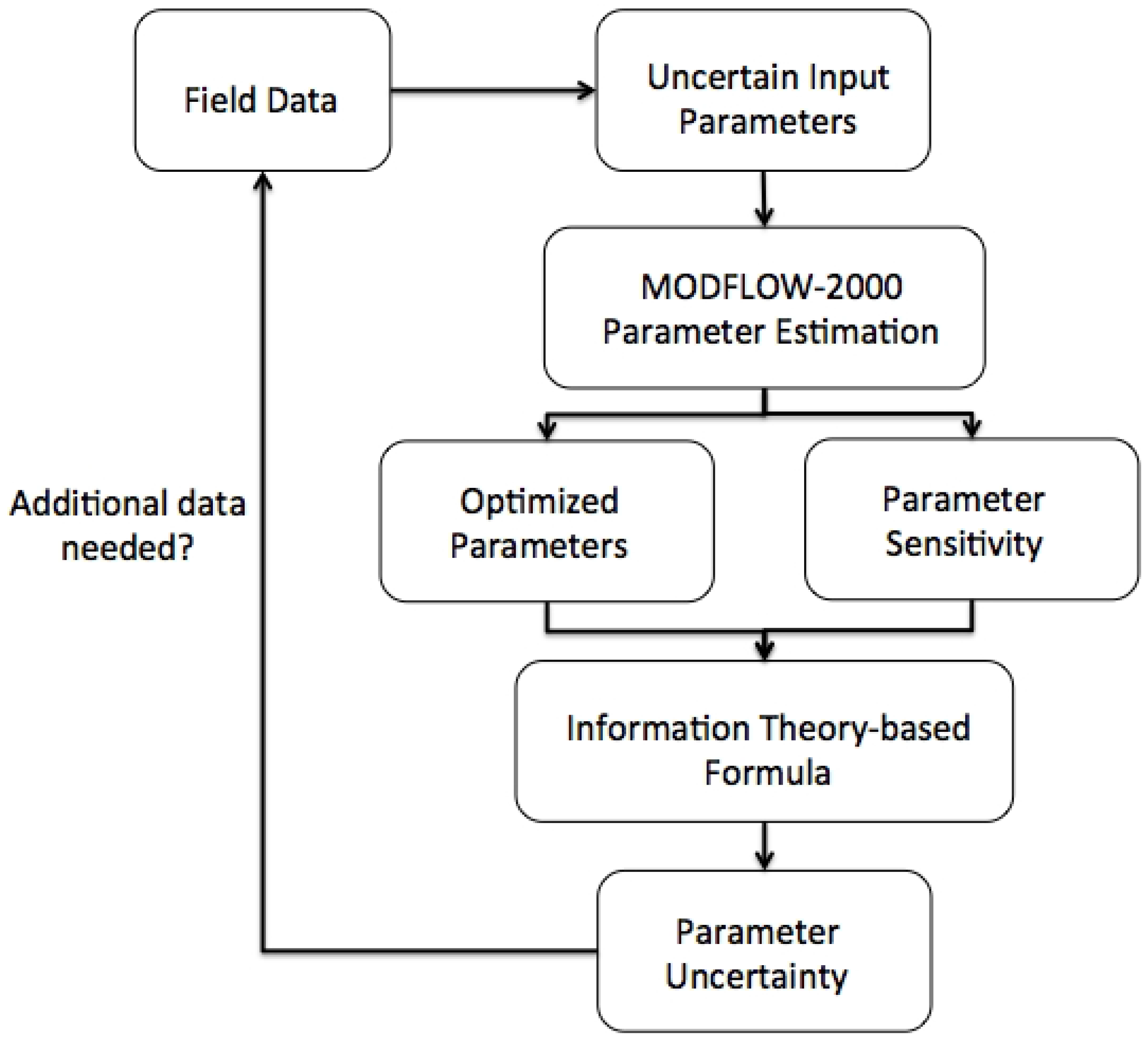
Figure 1.
Flowchart of ITb approach using MODFLOW-2000.
Figure 1.
Flowchart of ITb approach using MODFLOW-2000.
Two constraints are introduced to obtain unbiased probability
ρ(
x). The first constraint is the normalization constraint:
This is the basic constraint stating that the sum of the probabilities of all possible states in a system should be equal to one. The second constraint is the error constraint associated with the error from available data. For example, if hydraulic heads constrain a ground flow model, the error function
E(
x) becomes zero as the difference between observed heads and simulated heads goes to zero. Associating
E(
x) with
ρ(
x), the expected error
E* is given by:
In groundwater modeling,
E* can be the observation errors such as spurious fluctuations of head or conceptual model errors. To construct
ρ(
x),
S is constrained by Equations (2) and (3) using Lagrange’s method [
21]. The detailed mathematical calculation is described in the
Appendix. The probability
ρ(
x) for the most probable state of
x is:
where
Np is the number of model parameters,
Hx[
E(
x)] is the Hessian matrix for
E(
x),
λi is the eigenvalue of
Hx[
E(
x)],
Emin is the global minimum of
E(
x), Δ
x is the perturbation vector on
x, and Δ
xT is the transpose of Δ
x.
Implementation of Equation (4) starts with parameter optimization. After the parameters of interest are optimized at
Emin, the Hessian matrix
Hx[
E(
x)] and its eigenvalues are calculated around the optimized parameter
x using a finite-difference approximation method [
20]. For multivariate cases, the covariance of parameters can be obtained from the Hessian matrix. In the Gaussian domain, the multivariate probability density function is given as:
where
xm is the mean vector;
C is the covariance matrix of
x; and det
C is the determinant of
C [
22]. As
x →
xm , the covariance
C is obtained by:
where
is the inverse matrix of
Hx[
E(
x)]. Mathematically,
E* should be greater than
Emin because the Hessian matrix should be positive-definite at a minimum. However, in practical usage, this condition may not be satisfied as
E* is dependent upon the data constraining the model. If the optimization goal is to have the minimum difference between
E* and
Emin, the absolute difference between
E* and
Emin can be used in Equation (4). Since Equation (4) is an analytic equation of
ρ(
x), it is compatible with any optimization technique and any groundwater model.
We adopted a finite difference approximation method [
20] to obtain second-order derivatives of functions for the Hessian matrix. For the diagonal elements of the Hessian matrix, centered difference approximation for a univariate function
was used:
where
is the second-derivative of
for a given small value of
. The off-diagonal elements of the Hessian matrix are in a form of bivariate function
and its second-order derivative function is:
where
is the second-derivative of
for given small values of
and
for variables of
and
, respectively.
6. Synthetic Model Application
We adopted an example case cited in [
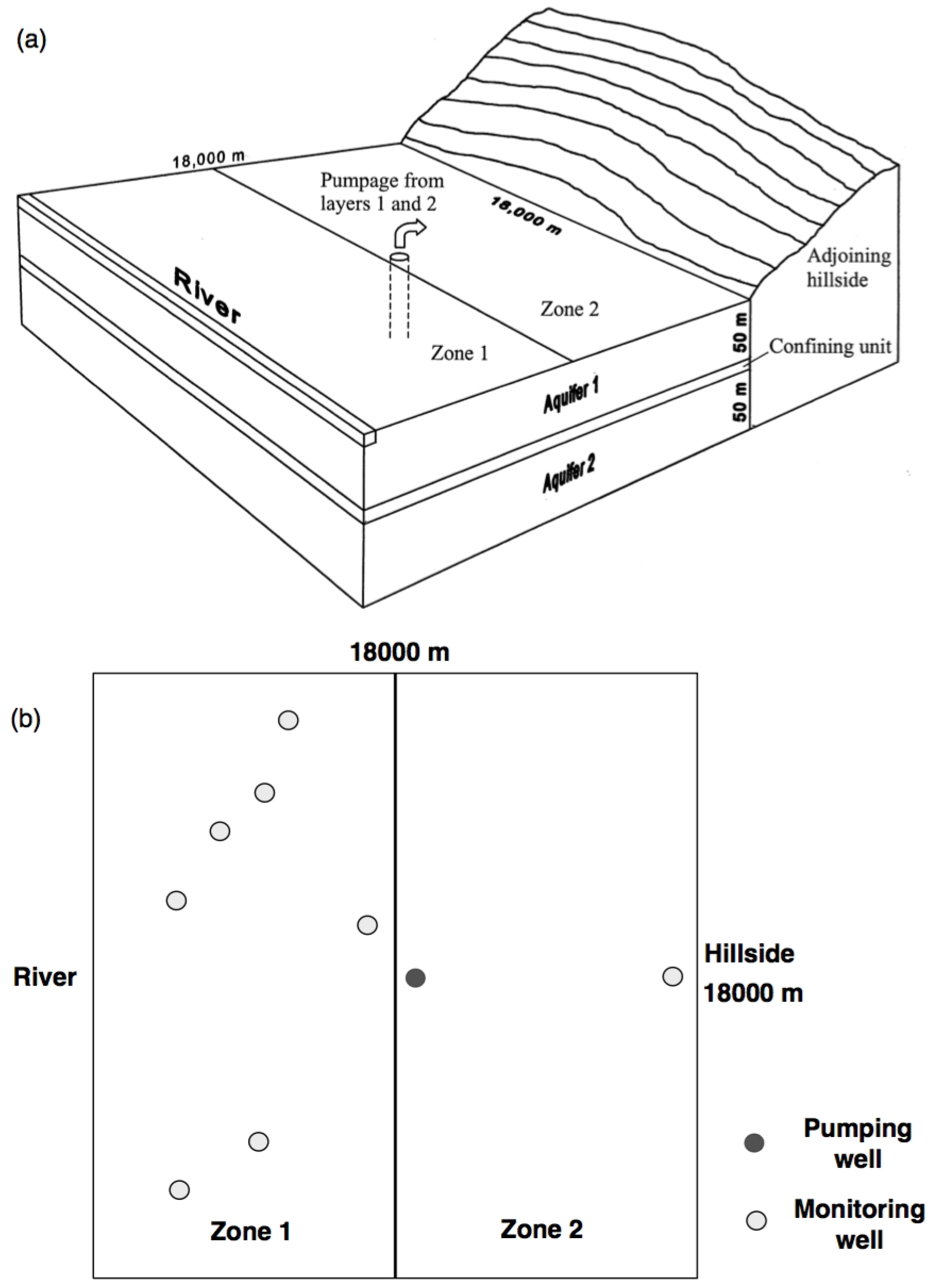
19] to verify validity of the ITb approach. The setup for this synthetic model is shown in
Figure 2. The system consists of two confined aquifers, each 50 m thick. The upper aquifer is labeled as Aquifer 1 and the lower one as Aquifer 2. A 10 m thick confining unit separates the two confined aquifers. A river flows west of this system and is hydraulically connected to Aquifer 1. To simulate the river, the entire west boundary is treated as a head-dependent boundary fixed to the constant value of 100 m. Towards the east is an adjoining hillside, which is a major contribution to the recharge of the system. This recharge is assumed to be known and hydraulically connected to both the Aquifers 1 and 2. A constant head boundary of 100 m is set along the east side of the system representing a flow divide. Areal recharge to Aquifer 1 is divided into two equal zones. Zone 1 is closer to the river and Zone 2 is farther away from the river. No flow boundaries are set up on the north and south sides. Wells are present in the studied area as shown in
Figure 2b. There is one well, centrally located, that is assumed to pump water with the same flow rate from both the aquifers. The model has an area of 18,000 m by 18,000 m and is discretized into 1,000 m by 1,000 m sized squares so that the grid has 18 rows and 18 columns. For the finite-difference method, time discretization is specified to simulate the model for a steady state period followed by a transient state period. The steady state period has no pumping and is simulated with one stress period having one time step. The transient period has a constant pumping rate and is simulated with four stress periods having one time step. The first three stress periods are 1, 3, and 6 days long, and each has one time step; the fourth is 272.8 days long and has 9 time steps, and each time-step length is 1.2 times the length of the previous time-step length [
19]. Other parameters and their values are listed in
Table 1 and model input files are provided in [
19].
Figure 2.
The synthetic model setup. (
a) The original schematic setup in Hill
et al. [
19]. (
b) Plan view of the synthetic model setup.
Figure 2.
The synthetic model setup. (
a) The original schematic setup in Hill
et al. [
19]. (
b) Plan view of the synthetic model setup.
Table 1.
Input parameters for the synthetic model.
Table 1.
Input parameters for the synthetic model.
| Parameter | Value |
|---|
| Recharge in Zone 1, RCH_1 | 0.63 m/yr |
| Recharge in Zone 2, RCH_2 | 0.32 m/yr |
| Storage coefficient of Aquifer 1, SS_1 | 1.3 × 10⁻³ |
| Storage coefficient of Aquifer 2, SS_2 | 2.0 × 10⁻⁴ |
| Vertical hydraulic conductivity of confining layer | 1.0 × 10⁻⁷ m/s |
| Hydraulic conductivity of riverbed | 1.2 × 10⁻³ m/s |
| Hydraulic conductivity of Aquifer 1, HK1 | 3.0 × 10⁻⁴ m/s |
| Hydraulic conductivity of Aquifer 2, HK2 | 4.0 × 10⁻⁵ m/s |
| Pumping rate in each layer 1 and 2 | 1.10 m3/s |
| Hydraulic head of river | 100 m |
The parameters in
Table 1 are considered as uncertain parameters in [
19]. In the present application of ITb, the hydraulic conductivity of Aquifer 1, HK1 and that of Aquifer 2, HK2 are the two target parameters to be optimized while other parameter values are fixed. The observed hydraulic heads are obtained from the sampling wells shown in
Figure 2. The starting values, true values and optimized values of HK1 and HK2 are listed in
Table 2. The minimum error E
min, which is the sum of squared, weighted residual of MODFLOW-2000 at the optimized state, was 43.37 (unitless). After running MODFLOW-2000, we applied the ITb to generate the Hessian matrix and its eigenvalues by perturbing the hydraulic conductivities for the hydraulic heads. The results of the ITb calculation are shown in
Table 3. The value of the expected error, E
* is assumed to be 100 (unitless).
Table 3 shows that the standard deviation of HK1 is almost ten times greater than that of HK2, which may imply that HK1 is more uncertain than HK2. However, this may not be true as the optimized values of HK1 and HK2 are also an order of magnitude apart. To avoid the scale difference the coefficient of variation was calculated for each parameter as listed in
Table 3. The coefficient of variation shows that HK1 is still more uncertain than HK2. The correlation coefficient is −0.76 suggesting that HK1 and HK2 are closely related in opposite direction of change, so that an increase in one will result in a decrease in the other and vice versa.
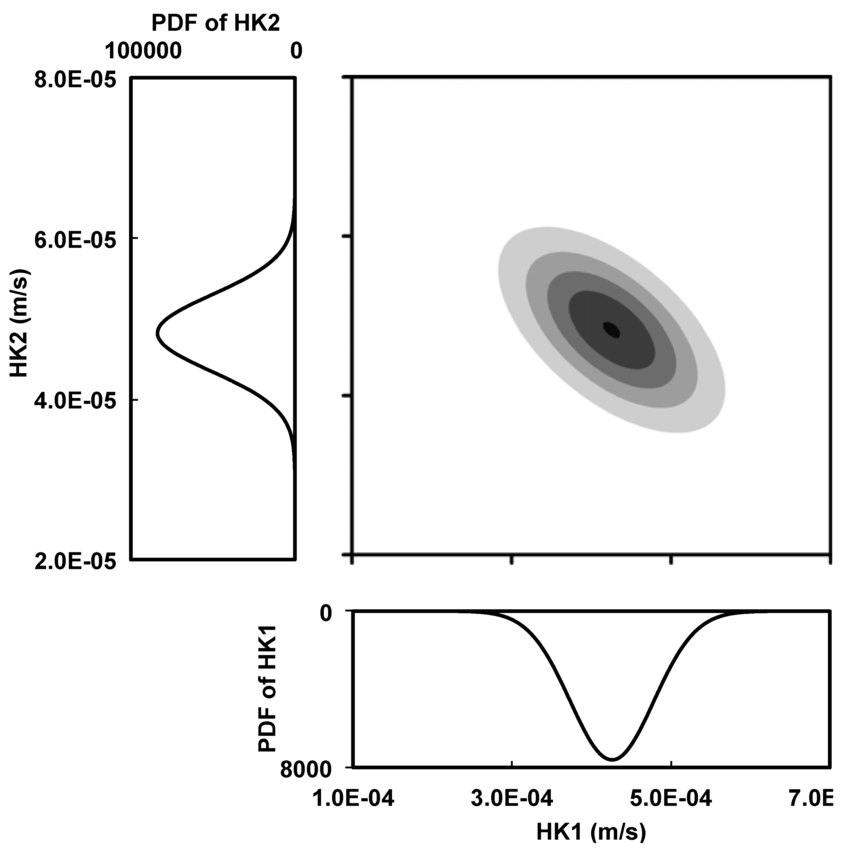
Figure 3 shows the bivariate probability density function (PDF) and univariate PDFs for HK1 and HK2 using the variance in Equation (6). The univariate PDFs indicate that the true values of HK1 and HK2 are located within the range of standard deviation around the optimized values. This proves that for the given head observations, the optimization process of MODFLOW-2000 is successful in estimating HK1 and HK2.
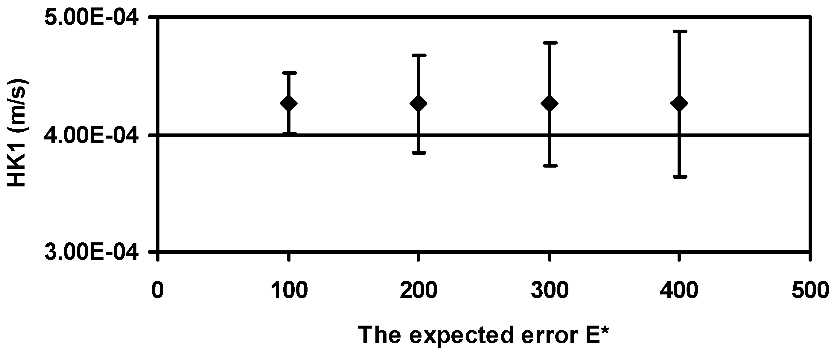
Figure 4 shows the change of parameter uncertainty with respect to the different expected errors. If the expected error is much greater or smaller than the global minimum, then the uncertainty increases. The bars represent the standard deviation of HK1. It is clearly shown that as the expected error increases, there is a subsequent increase of the parameter uncertainty.
Table 2.
Parameter values after optimization process of MODFLOW-2000.
Table 2.
Parameter values after optimization process of MODFLOW-2000.
| Parameter | True Value | Starting Value | Optimized Value |
|---|
| HK1 (m/s) | 4.0 × 10⁻⁴ | 3.0 × 10⁻⁴ | 4.26 × 10⁻⁴ |
| HK2 (m/s) | 4.4 × 10⁻⁵ | 4.0 × 10⁻⁵ | 4.82 × 10⁻⁵ |
Table 3.
Statistical outputs of the synthetic model.
Table 3.
Statistical outputs of the synthetic model.
| Parameter | Standard Deviation (m/s) | Coefficient of Variation (Unitless) |
|---|
| HK1 | 5.25 × 10⁻⁵ | 10.23 × 10⁻² |
| HK2 | 4.76 × 10⁻⁶ | 9.88 × 10⁻² |
Figure 3.
The bivariate probability density function (PDF) and univariate PDFs for HK1. and HK2.
Figure 3.
The bivariate probability density function (PDF) and univariate PDFs for HK1. and HK2.
Figure 4.
Parameter uncertainty of HK1 for the expected error E*. The bars indicate the standard deviation of HK1.
Figure 4.
Parameter uncertainty of HK1 for the expected error E*. The bars indicate the standard deviation of HK1.
7. Case Study: Kansas City Plant
The Kansas City Plant (KCP) is located 12 miles south of downtown Kansas City, Missouri. It was established in 1942 and occupies approximately 141 acres of the 300-acre Bannister Federal complex. The KCP is responsible for production and procurement of non-nuclear components for nuclear weapons. The KCP does not perform any onsite waste disposal. Onsite sanitization is mainly for non-hazardous classified wastes. The hazardous wastes are sent offsite for treatment or disposal. The waste management operations at the plant mainly consist of storing these hazardous wastes until they are taken offsite. In addition to hazardous wastes, some low-level radioactive wastes are also generated. For national security reasons, some wastes are classified. Selective recycling and industrial wastewater pretreatment are the main treatment operations at the KCP [
23].
From the 1940s to the 1960s, a part of the northeast area (NEA) was used as a dumping site for waste from the KCP, resulting in extensive soil and groundwater contamination. Additional contamination from the release of polychlorinated biphenyl (PCB) and a man-made chemical, which was banned from U.S. manufacturing in 1979, continued through the early 1970s [
23]. The immediate concern was the contaminant plume getting into the Blue River (
Figure 5). The contaminant plume consisted of volatile organic compounds including trichloroethylene, 1,2-dichloroethylene, and vinyl chloride. To prevent migration of the contaminant to the Blue River, an interceptor trench was installed in 1990 and operated until 1998 to catch the plume. After extensive site investigation in 1998, a passive iron wall permeable reactive barrier (PRB) was installed to replace the interceptor trench. This passive iron wall was not successful as the contaminant bypassed the southern end of the wall. The groundwater flow simulation predicted that containment of the contaminant would require pumping rates in excess of 30 gallons per minute (gpm). The existing interceptor trench tried to contain the contaminant by pumping at a rate of 6 gpm, hence the modeling design was discarded and further hydrological analysis of the NEA groundwater flow system was made [
23]. To characterize the groundwater flow system, [
23] collected data from 28 newly installed temporary wells and the existing monitoring wells, 12 stilling wells, four mini-piezometers, and a weir. Recharge from the cattail drainage was found to cause groundwater mounding, which deflected the plume to the east soon after entering the lower NEA (
Figure 5). This mound was considered to be a consistent hydrologic feature because of the frequent storm events in Kansas City. The plume in the vicinity of the iron wall was more than 60 m wide.
For the ITb application we divided the area of study into 50 by 50 cells that are 4.42 m by 4.16 m giving us an area of approximately 221 m in the east-west direction and 208 m in the north-south direction. The geology consists of alluvial sediments overlaying impervious shale. The alluvial aquifer in the lower NEA consists of a 4.57 to 7.62 m thick upper clayey-silt layer underlain by a 0.30 to 1.52 m thick basal gravel layer. The contrast of hydraulic conductivities in these two layers made the potentiometric surface of the more permeable basal gravel layer 0.3 m to 0.6 m lower than the potentiometric surface in the less permeable clayey-silt, creating a downward hydraulic gradient. For modeling purposes we considered the clayey-silt layer and the basal gravel layer to be of average thickness 5.49 m and 0.91 m, respectively, with average hydraulic conductivities of 0.23 m/day and 10.36 m/day, respectively. The dimensions of the interceptor trench were 4.57 m wide, 65.53 m long and 9.14 m deep. The iron wall PRB was designed such that it was 0.6 m wide in the 5.5 m deep upper clayey-silt layer and 1.83 m wide in the basal gravel layer, with a length of 39.62 m and hydraulic conductivity ranging from 91.44 to 152.4 m/day.
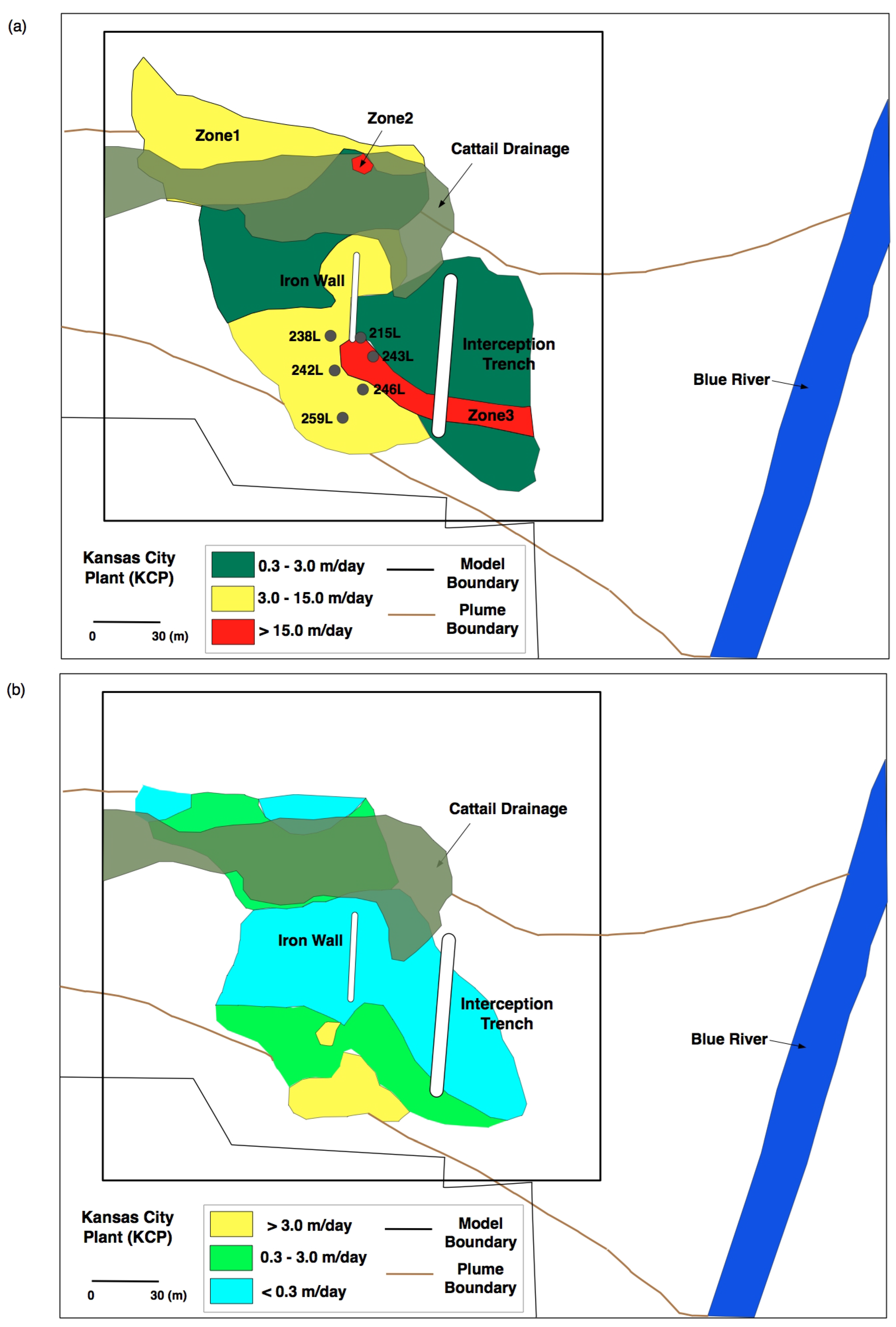
Figure 5.
The hydraulic conductivity distribution for the KCP site (modified from [
23]). Each zone of hydraulic conductivity is defined with a closed boundary and different color. (
a) The lower basal gravel layer. (
b) The upper clayey silt layer.
Figure 5.
The hydraulic conductivity distribution for the KCP site (modified from [
23]). Each zone of hydraulic conductivity is defined with a closed boundary and different color. (
a) The lower basal gravel layer. (
b) The upper clayey silt layer.
In the KCP model, we adopted head observations from the 26 wells located in the model domain and used them for a steady state simulation; hence the stress period for all observations was 1. The hydraulic conductivity values were obtained from [
23] for the clayey-silt layer and the basal gravel layer. The hydraulic conductivity values from the wells in each zone were averaged and assigned as a zonal hydraulic conductivity for that zone. The SEN file had the hydraulic conductivities of the 18 zones in the model. The clayey-silt and the basal gravel layers had seven different hydraulic conductivity zones each (
Figure 5). The remaining four zones were used for the layer of peat or humus, the fill layer, and the areas around the clayey-silt and the basal gravel layers. The model was set up with no flow boundaries on the north and south boundaries. The west boundary had a constant head boundary while the east boundary had no flow boundary. We assumed the vertical hydraulic conductivity to be 1/20 times that in the horizontal direction. The head change and residual convergence criteria were both taken as 1.0E-5 and no damping was set in the model.
The KCP case study [
23] listed the observed minimum and maximum hydraulic conductivities of all the wells in both the upper clayey-silt layer and the lower basal gravel layer. Among them the six wells having the largest difference of hydraulic conductivities are listed in
Table 4 and located in
Figure 5a. The well numbers with “L” stand for the lower basal gravel layer. Note that the difference between minimum and maximum hydraulic conductivities is up to nearly ten times that of the minimum value. During the PRB design process the averages of such highly variable hydraulic conductivities were adopted [
23]. Interestingly all the six wells are located south of the iron wall of PRB where the contaminant plume bypassed.
Table 4.
Pumping test results at six selected wells in
Figure 5.
Table 4.
Pumping test results at six selected wells in Figure 5.
| Well Number | Minimum Hydraulic Conductivity (m/day) | Maximum Hydraulic Conductivity (m/day) | Average Hydraulic Conductivity (m/day) |
|---|
| 215L | 30.96 | 149.81 | 89.88 |
| 238L | 23.86 | 238.59 | 131.23 |
| 242L | 24.91 | 249.06 | 136.98 |
| 243L | 21.88 | 54.71 | 38.30 |
| 246L | 20.19 | 201.89 | 111.04 |
| 259L | 23.89 | 119.45 | 71.67 |
For the ITb application, we targeted three zones having different hydraulic conductivities. We included the zone where the plume bypassed the PRB and also two other zones around cattail drainage having recharge of water that deflected the groundwater flow towards east and south. We limited the number of zones to just three because the complexity and computational time increases with addition of more zones. All three zones were located in the lower basal gravel layer as shown in
Figure 5(a). We named those as Zones 1, 2, and 3, respectively. The initial values for Zones 1, 2, and 3 were optimized using MODFLOW-2000 to give the best representation of model-to-site configuration. The minimum error from the MODFLOW-2000 was E
min = 32.37 (unitless). The standard deviation of the three parameters and their correlation coefficients along with initial and optimized hydraulic conductivities are listed in
Table 5. We assumed the expected error E
*to be 40 (unitless). It is shown that Zone 3 is the most uncertain of the three. As discussed in [
23], this zone has three to ten times higher hydraulic conductivity compared to the one used in the PRB design. The correlation coefficients show that there is almost no correlation between Zones 1 and 3, and Zones 2 and 3, while Zones 1 and 2 are negatively correlated, meaning that an increase of hydraulic conductivity in Zone 1 would lead to a decrease of hydraulic conductivity in Zone 2 and vice versa. If additional site exploration is required, Zone 3 would be the first area to be investigated since it has the most uncertain hydraulic conductivity estimation.
Table 5.
Optimized hydraulic conductivities and standard deviations for three zones of the Kansas City Plant (KCP) model.
Table 5.
Optimized hydraulic conductivities and standard deviations for three zones of the Kansas City Plant (KCP) model.
| Zone | Initial Hydraulic Conductivity (m/day) | Optimized Hydraulic Conductivity (m/day) | Standard Deviation (m/day) |
|---|
| 1 | 9.22 | 13.02 | 129.33 |
| 2 | 17.11 | 31.15 | 30.89 |
| 3 | 26.44 | 32.81 | 155.25 |


