4.1. Properties of the Kick
In
Section 2.3 we looked at a two level spin system passing through a Stern–Gerlach (SG) apparatus. Our purpose was to establish minimal requirements for
any kind of special state. Now however, we really want to consider the true physical system, the Stern–Gerlach experiment.
As emphasized, our usual perspective is
not to focus on the dynamics of this system alone, but rather on that of the entire environment necessary for a full description. The richness of the environment is what supports the existence of special states. However, in the present section and in the analysis of
Section 2.3, a different viewpoint is taken, closer to the way most quantum calculations are done. The environment is in whatever special state it is in, but because this state may be rare, its action on the particle or spin of interest will also be unusual. We focus on that action alone and treat the environment’s rare action through an effective Hamiltonian. This Hamiltonian provides the time evolution of the wave function through left multiplication by
.
The system is prepared by passing a beam of atoms through another Stern–Gerlach apparatus and only that part of the beam having a particular value of angular momentum, say
along a particular direction, is selected and sent on to the next SG apparatus. The second SG apparatus is not (necessarily) oriented in the same direction. Let the direction of motion (aside from the eventual deflection) be in the positive
y direction and the gradient of the second SG apparatus be in the
z direction. Let
, and
be unit vectors along the
, and
z axes, respectively. We assume that when entering the second apparatus—which is the one on which we focus—the atom’s spin is along the direction
, for some angle
θ. As in Equation (
5), the initial wave function of an atom, when exiting the first SG apparatus, can be taken to be
consistent with the preparation just specified. It is possible to multiply
by an arbitrary overall phase or to use density matrices, but this does not affect our conclusions. For the SG experiment the final state should have
(“
up”) or
(“
down”), which requires that the angle in Equation (
12) be rotated to become an integer multiple of
π. Thus the overall action of the effective Hamiltonian is to add an angle
ϕ to
so as to accomplish this goal [
22]. We refer to this action of the effective Hamiltonian as a “kick”. The kick is thus a left multiplication of the wave function by
bringing it to
up or
down. As indicated, the effective Hamiltonian in Equation (
13) represents the effect of uncontrollable elements of the environment.
As discussed in
Section 2.3 (and proved in Section 9.1 of Reference [
1] or [
23], Section 4.1) recovery of the Born probabilities requires that the kicks be Cauchy distributed, namely that the probability density for a kick of size
ϕ should be
with
a a parameter that is small. Moreover, it is a property of this distribution that the least unlikely way to achieve large (compared to
a) total rotation of the spin is through a single kick.
For
up we thus require
and for
down , with
. Define
Then the probability for the two outcomes is
with
Z, the sum of
F at the two values, providing normalization. For small
a this recovers the standard probabilities. The sums can be done explicitly, but we hold off, since there will be related sums to evaluate and we will do all of them at once.
In searching for evidence of special states, presumably the larger the kick the larger the signal. With this in mind, we calculate the expectation of kick size both conditioned on an outcome and unconditioned. We thus want
and their sum.
To evaluate Equations (
15), (
17) and (18) consider the following identity [
24]
where
n runs over the integers. The poles of one over the tangent function occur at multiples of
π and the residues are unity. Let
. Using elementary relations we write the real and imaginary parts of Equation (
19),
From Equation (21) we get the following information:
and for sufficiently small
a,
, as it should.
Remark 1: As mentioned in
Section 2.3 and explicitly calculated in [
1,
23], for
a not negligible there will be a deviation from standard probabilities. This imposes a restriction on
a, but does not provide an experimental test since, in the absence of physical specifics, there is no information on the size of
a.
Equation (
20) gives the sums used in the expectations of the kick-angles and yields
If
there is no specializing, so the expected kick size for those measured as
up goes to zero. Surprisingly perhaps for those measured as
down the expectation is even smaller. This is because although the kicks (however few) are larger, they are as likely to be positive as negative.
According to Equations (
22) and (23) the average kick size is order unity, although given the quirks of the Lévy distributions, this was not a foregone conclusion. Looking at Equations (17) and (18) it is clear that moments higher than the first do not exist (the first moment is borderline), so that it is conceivable that with experimental studies that focus on large kicks other information may be gleaned.
Remark 2: Three of the series that we have considered, Equations (17), (18) and (19), are only conditionally convergent. As Hille [
24] remarks in connection with Equation (
19), one can add
(
) to each summand to obtain absolute convergence, or what is essentially the same thing, choose to combine positive and negative
n terms before summing the infinite series.
Remark 3: If one performs a series of experiments and manages to measure the kick in each of them, the average will not converge to the results of Equation (
22) or Equation (23). This is where the “quirks” of the Lévy distribution enter. As remarked, some of our series are not absolutely convergent and the distribution is not self-averaging. In fact the average of many measurements has the same probability distribution as a single measurement. This can be useful for the experimentalist looking for the effect, since even with averaging there is no suppression of large magnitude kicks. The use of the average might be thought of as the setting of the scale but in fact the only scale is
a, which is taken to be small. By conditioning on large events,
a disappears and there is really no scale.
Depending on experimental setup, it is possible to optimize the angle for maximum signal. For example, suppose one is able to sort particles according to outcome. Then to optimize as a function of θ, one would consider the strength of the field needed for (say) up, times the probability of up. This is proportional to . The derivative of this function, , vanishes for and . Both are stationary points, but the maximum is the second value, . On the other hand, one may send in a large number of particles and simply want to maximize the (absolute value of) the total, . This gives which has a shallow minimum at and maxima symmetric about this minimum, one of them being at .
It follows that there is not a lot of profit in fine tuning the optimization. However, what is more significant is that there is a definite θ dependence. Thus if θ is varied between 0 and one could compare a no-signal situation (no special state is needed) with a positive signal situation, say at .
4.1.1. Strength of the Field Inducing the Kick
For a spin about to enter a Stern–Gerlach apparatus, the effective part of
of Equation (
13) involves a magnetic field,
. For the kick angle
ϕ to have characteristic size unity we require
where
is the duration of the field’s interaction with the spin. The quantity
μ is essentially the electron magnetic moment; taking its magnitude to be the Bohr magneton, implies
To evaluate
B requires an estimate of
, in turn requiring some picture of the nature of the interaction. At this stage, two possibilities present themselves. The field may be connected to the strong magnetic field the atom experiences in approaching and passing through the magnets. Or the field could be something separate, carried perhaps by an externally arriving photon.
We first consider a possible association with the SG field. A conservative estimate would be interaction durations of a few ms, in which case field strengths would be about T, which is well within the range of macroscopic measurement. However, this is probably too conservative. In a typical SG experiment the Ag or K atoms are moving at about 1 km/s. If the kick takes place within about 10cm, then s and the field strength would be on the order of 0.1 G, something your compass needle could discern.
As far as an electric field generated by this transient field, Maxwell’s equations suggest , where L is the characteristic scale for the spatial variation of E and T the time scale for variation of B. If m and s, we find an electric field on the order of V/m, also easily measurable. Another estimate in this connection uses km/s. Thus .
Now consider an outside photon, not necessarily related to the magnetic fields of the SG apparatus. An estimate of this photon’s energy can be made in terms of the time of interaction: since
is an energy, by Equation (
24) that energy should be roughly
. If
is a characteristic electromagnetic interaction time,
s, this gives an energy on the order of 5 eV.
4.1.2. Magnetic Fields along the Particle Path
A convenient way to study the field in the Stern–Gerlach apparatus [
25] is to replace the magnets (for purposes of calculation) by a pair of infinite parallel wires with currents flowing in opposite directions. The magnitude of the field is then constant on (circular) cylindrical surfaces for distances large in comparison to the wire separation. This matches the field seen by the passing particle if the pole pieces have the shape of those cylinders. As desired, this magnetic field has a steep gradient perpendicular to the cylindrical surfaces.
Our interest is not so much in the field within the magnet as the field seen by the atom as it approaches the magnet, moving in the positive
y direction. This will certainly depend on the specifics of the magnet, but to get a handle on those fields and to go beyond dimensional analysis, we study the
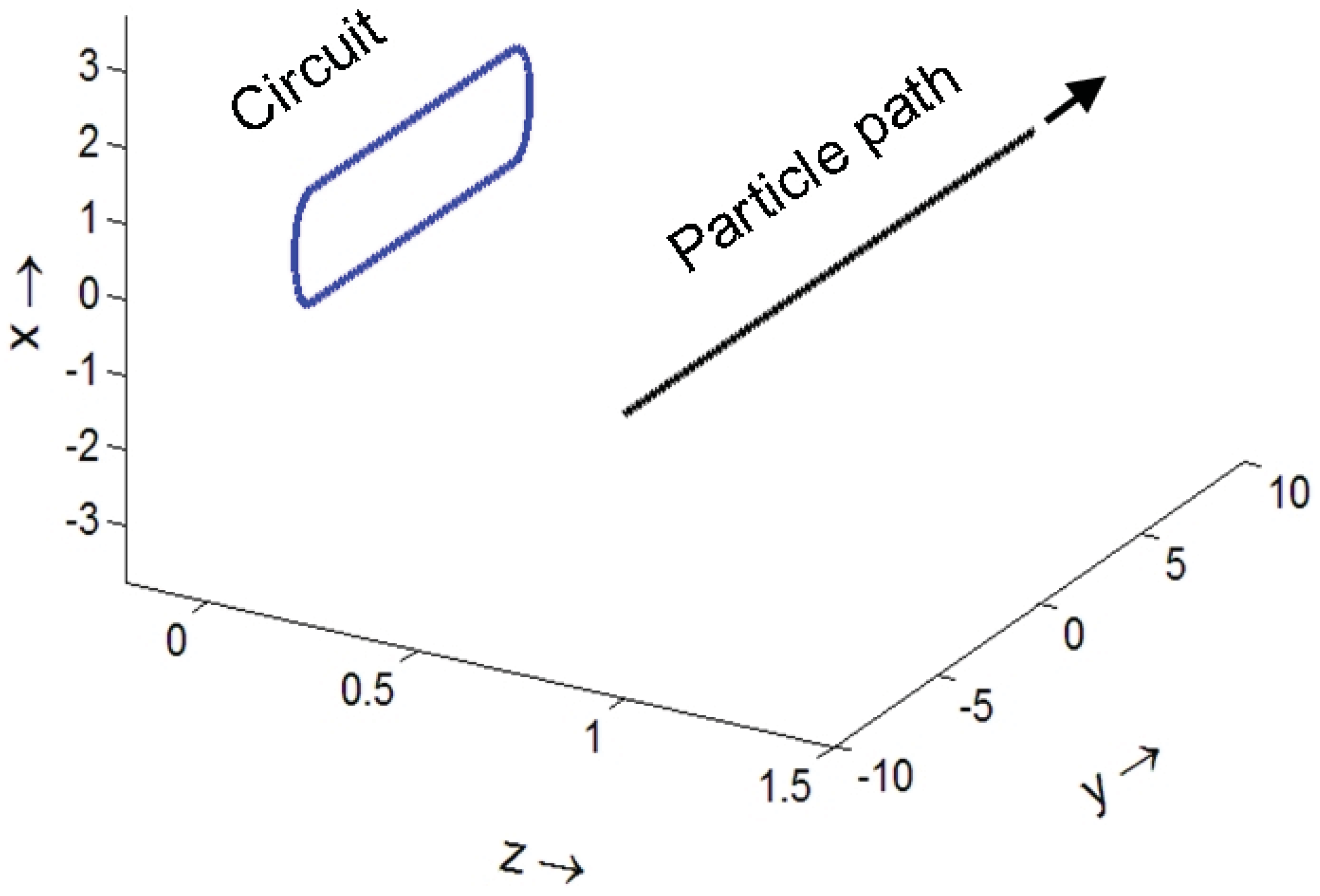
finite length magnetic field by simulating the actual field by one generated by a current loop that consists of two wires, but now they are finite. They extend for the length of the magnet and are joined at each end by a semicircular loop (completing the circuit).
Figure 8 illustrates the following geometry: The circuit is in the
x-
y plane (
). The straight-wire portions run from
to
, the upper portion at
, the lower one at
. The semicircles at each end (also in the
x-
y plane with
) are of radius
s. The particle trajectory is in the direction of increasing
y and parallel to the
y-axis. It has
and a value of
z large enough so that in its neighborhood the contour lines of the field are essentially circles in the
x-
z plane. The field at a point
is given by the following integral:
where
I is the current and SI units are used. Now the particle
is deflected in the positive or negative
z direction (that’s the point of the experiment). But there will also be some spread of the beam in the
x direction whose consequences for the field we will evaluate to lowest order. The contour, Γ, consists of four parts, the top (“T”) portion of the wire parallel to the
y axis, the bottom (”B”) portion, the right semicircle (“R”,
) and the left semicircle (“L”,
). For
(which is the plane
), the straight wire portions can be fully integrated and give
where
. We also present the first order correction for small
x,
i.e., the observation point
becomes
. The additional term is of the form
. After a bit of calculation one obtains
where
(± implicit on
A and
λ), with
and
. Because of the
z dependence, vertical (
x) spread in the beam will cause (unwanted) blurring of the spin-induced splitting.
Figure 8.
Geometrical configuration. The separation of the wires is 2s. The particle moves in the positive y direction in the plane and at a positive, essentially constant z value that is larger than s. Looking at the circuit from positive z, Equation (27) corresponds to a current moving in the clockwise direction.
The field from the two semicircular portions does not have a general closed form solution but analytic information can still be obtained. The length of the path within the magnet, L, will be assumed long enough so that we need consider only one semicircle at a time. Moreover, with respect to the SG apparatus on which we focus (the second) the field on exit is irrelevant, since at that stage only location is measured, not spin. Nevertheless, the exit field will play a role for the first apparatus, because it can change what we assume is the incoming state. Qualitatively though, the possible effects will be the same.
A point on the semicircular portion of the wire near
is given by
, with
ψ running from 0 to
π. For clockwise circulating current (as viewed from positive
z)
is in the direction of the current. After a bit of calculation we obtain an expression for the left semicircular (“L”) contribution
where
. For purposes of studying the effective Hamiltonian, Equation (13), we are only interested in the
x-component of this field. Specializing to
, the integral can be performed, yielding
As the atom approaches the magnet, this field rotates the spin one way and then the other. The magnitude of this field is substantial. Rewrite the field as
The dimensionless quantity in the square brackets has a maximum of about
for
, which is approximately the value in the experiment of Reference [
25]. Comparing Equation (27) and Equation (31) it is seen that the external field reaches almost half the field value inside the magnets.
4.2. Detection Scenarios
The general strategy is to send in atoms with spins at (say) 50° relative to the
z-axis (tilted along the
y-axis) and to send them in at 0° [
26]. Comparison of the two cases should show additional “random” activity—noise—when they are at the non-zero angle. At 0° no kicks are necessary to drive the spins into a single beam for the SG experiment. At 50° they will all need to be sent one way or the other. The actual rotating of the spins would not itself be visible, but related and additional fields should be present. The idea is that there should be “collateral damage”, by which is meant that the photon or field fluctuation is not perfectly matched to accomplish its rotational task and nothing more. As discussed at length in Reference [
1], in generating a special state one seeks the
least unlikely of them. A fundamental assumption in the present proposal is that a perfect match is less likely than an imperfect one. In addition, by virtue of Maxwell’s equations, there are compulsory electric fields alongside the magnetic fields that rotate the spin.
Ways to fine-tune the strategy above may certainly exist. For example, if the signal of a kick can be correlated with a particular atom (which goes either up or down), differences in signal rates for different angles can be further exploited.
4.2.1. Scenario when the Fields Are Generated by the SG Magnets
One issue is the stability of the fields. The fields needed for rotating the spins are on the order of 1G, while the magnet is maintaining a field of roughly 5000 G. One thus needs field measurements with better than 0.1% accuracy. It should also be recalled that the preparation of the spin at some particular angle is accomplished by means of a earlier SG setup. Kicks can occur in the first as well as the second magnet. The rotating fields for the magnets (meaning, for the example studied, fields in the
x-direction) are also different for different atoms because of finite beam width (
cf. Equation (
31) where there is
z-dependence in the field).
Furthermore, the magnetic fields that can rotate the spin are necessarily accompanied by electric fields since the variety of rotation directions through the magnet (for ) demands time-dependent variation of . With an atomic velocity of 1 km/s, a conservative estimate puts these fields on the order of 1 or more V/m.
For an atomic beam, there may be additional effects. Many atoms pass through the magnet at roughly the same time. Not all of them are rotated the same way, so that rapid variation of the magnetic field would be required (along with the electric fields just discussed). In addition, the “least unlikely” principle suggests that there would be a tendency for bunching in the output, that is there would be short-time correlations in up or down outcomes. The rationale is that a single large fluctuation is more likely than two independent ones.
4.2.2. Scenario when the Fields Are Generated by External Photons
Our rough estimate for photon energy was in the eV range, visible or UV light when the kick drives the spin around many times (as is occasionally expected, given the Cauchy distribution). Individual photons in this energy range should be easy to detect.
It should be pointed out though that the estimates of
Section 4.1.1 are only that—estimates. A general scale is established. However, the properties of the Cauchy distribution imply that this scale will often be vastly exceeded. For this reason I do not go beyond the semiclassical assumption, implicit in that calculation, that the field acts on the atom, but not vice versa. For atom-photon scattering one should in principle work in a QED context. My assumption is that both incoming photon and outgoing photon will all be on the scale of the estimate.
