1. Introduction
Uncertainty regarding statistical models and associated estimating equations and the data sampling-probability distribution function create unsolved problems as they relate to information recovery. Although likelihood is a common loss function used in fitting statistical models, the optimality of a given likelihood method is fragile inference-wise under model uncertainty. In addition the precise functional representation of the data sampling process cannot usually be justified from physical or behavioral theory. Given this situation, a natural solution is to use estimation and inference methods that are designed to deal with systems that are fundamentally stochastic and where uncertainty and random behavior are basic to information recovery. In this context [
1,
2], the family of likelihood functionals permits the researcher to face the resulting stochastic inverse problem and exploit the statistical machinery of information theory to gain insights relative to the underlying causal behavior from a sample of data.
In developing an information theoretic approach to estimation and inference, the Cressie-Read (CR) family of information divergences represents a way to link the model of the process to a family of possible likelihood functions associated with the underlying sample of data. Information divergences of this type have an intuitive interpretation reflecting the uncertainty of uncertainty as it relates to a model of the process and a model of the data. These power divergences give new meaning to what is a likelihood function and what is the appropriate way to represent the possible underlying sampling distribution of statistical model.
One possibility for implementing this approach is to use estimating equations-moment conditions (prior information) to model the process and provide a link to the data. Discrete members of the CR family are then used to identify the weighting of the possible underlying density-likelihood function(s) associated with the data observations. The outcome reflects, in a probabilistic sense, what we know about the unknown parameters and possible density functions. In the case of a stochastic system
in equilibrium, the process may be modeled as a single distribution within the CR framework. An advantage of this approach, in addition to its divergence-optimality base, is that it permits the possibility of flexible families of distributions that need not be Gaussian in nature. For discussions relative to the flexible family of distributions, under given values of moments and indirect noisy sample observations, see [
3,
4,
5,
6,
7].
The paper is organized as follows: in
Section 2 we discuss the CR family of divergence measures (DMs) and relate these DMs to the maximum likelihood (ML) principle. Given the framework developed in
Section 2,
Section 3 is concerned with developing a loss basis for identifying the probability space associated with data observations. In
Section 4, the results of a sampling experiment are presented to illustrate finite sampling performance. Finally, in
Section 5 we summarize extensions to the CR-Minimum Divergence (MD) family of estimators and provide conclusions and directions for future research.
2. Minimum Power Divergence
In identifying divergence measures that may be used as a basis for characterizing the data sampling process underlying observed data outcomes, we begin with the family of divergence measures proposed by [
1,
2]. In the context of a family of goodness-of-fit test statistics (see [
7]), Cressie and Read (CR) proposed the following power divergence family of measures:
In (1), the value of indexes members of the CR family, represent the subject probability distribution, the
qi′s are reference probabilities, and
p and
q are
vectors of
pi′s and
qi′s, respectively. The usual probability distribution characteristics of
pi,
qi ∈ [0,1] ∀
i,
, and
are assumed to hold. The CR family of power divergences is defined through a class of additive convex functions that encompasses a broad family of test statistics, and represents
a broad family of likelihood functional relationships within a moments-based estimation context, which will be discussed in
Section 2.3. In addition, the CR measure exhibits proper convexity in
p, for all values of and
q, and embodies the required probability system characteristics, such as additivity and invariance with respect to a monotonic transformation of the divergence measures. In the context of extremum metrics, the general CR family of power divergence statistics represents a flexible family of pseudo-distance measures from which to derive empirical probabilities.
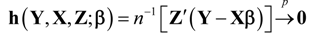
The CR statistic is a single index family of divergence measures that can be interpreted as encompassing a wide array of empirical goodness-of-fit and estimation criteria. As γ varies, the resulting estimators that minimize power divergence exhibit qualitatively different sampling behavior. Using data consistent empirical sample moments-constraints such as
![Entropy 14 02427 i002]()
, where
are respectively a
,
,
vector/matrix of dependent variables, explanatory variables, and instruments, and the parameter vector
is the objective of estimation, a solution to the stochastic inverse problem, based on the optimized value of
I(
p,
q,γ), is one basis for representing a range of data sampling processes and likelihood function values.
To place the CR family of power divergence statistics in an entropy perspective, we note that there are corresponding [
8,
9,
10] families of entropy functionals-divergence measures. As demonstrated by [
6], over defined ranges of the divergence measures, the CR and entropy families are equivalent. Relative to [
8,
9,
10], the CR family has a more convenient normalization factor
and has proper convexity for all powers, both positive and negative. The CR family allows for separation of variables in optimization, over the range of
, when the underlying variables belong to stochastically independent subsystems, called the
independent subsystems property [
6]. This separation of variables permits the partitioning of the state space and is valid for divergences in the form of a convex function.
2.1. The CR Family and Minimum Power Divergence Estimation
In a linear model context, if we use (1) as the goodness-of-fit criterion, along with moment-estimating function information, the estimation problem based on the CR divergence measure (CRDM) may, for any given choice of γ, be formulated as the following extremum-type estimator for
β: where
q is taken as given, and
denotes the appropriate parameter space for
β. Note in (2) that
and
denote the
rows of
and
, respectively. This class of estimation procedures is referred to as
Minimum Power Divergence (MPD) estimation and additional details of the solution to this stochastic inverse problem are provided in the sections ahead. The MPD optimization problem may be represented as a two-step process. In particular, one can first optimize with respect to the choice of the sample probabilities,
p, and then optimize with respect to the structural parameters
β, for any choice of the CR family of divergence measures identified by the choice of γ, given
q.
It is important to note that the
family of power divergence statistics defined by (1), is symmetric in the choice of which set of probabilities are considered as the subject and reference distribution arguments of the function (2). In particular, as noted by [
11,
12], whether the statistic is designated as
I(
p,
q,
γ) or
I(
q,
p,
γ),
the same collection of members of the family of divergence measures are ultimately spanned, when considering all of the possibilities for γ ∈ (−∞,∞)
2.2. Popular Variants of
Three discrete CR alternatives for , where , have received the most attention in the literature, and to our knowledge these are the only variants that have been utilized empirically to date. In reviewing these, we adopt the notation , where the arguments and are tacitly understood to be evaluated at relevant vector values. In the two special cases where , are to be interpreted as the continuous limits, , and , respectively.
If we let
, the reference distribution is the empirical distribution function (EDF) associated with the observed sample data, and also the nonparametric maximum likelihood estimate of the data sampling distribution. Minimizing
is then equivalent to maximizing
and leads to the traditional maximum empirical log-likelihood (MEL) objective function. Minimizing
is equivalent to maximizing
, and leads to the maximum empirical exponential likelihood (MEEL) objective function, which is also equivalent to [
13] entropy. Finally, minimizing
is equivalent to maximizing
, and leads to the maximum log-Euclidean likelihood (MLEL) objective function. Note the latter objective function is also equivalent to minimizing the sum of squares function
.
With regard to MPD (
family) estimators, under the usual assumed regularity conditions, all of the MPD estimators of
β obtained by optimizing the are consistent and asymptotically normally distributed. They are also asymptotically efficient, relative to the optimal estimating function (OptEF) estimator [
14], when a uniform distribution, or equivalently the empirical distribution function (EDF), is used for the reference distribution. The solution to the constrained optimization problem yields optimal estimates,
and
, that cannot, in general, be expressed in closed form, and thus must be obtained using numerical methods.
2.3. Relating Minimum Power Divergence to Maximum Likelihood
The objectives of minimizing power divergence and maximizing likelihood are generally not equivalent. However, two of the historical variants presented in the preceding section have direct conceptual linkages to maximum likelihood concepts, and the third is an analog to least squares. The traditional MEL criterion
coincides with the estimation objective of maximizing the joint empirical log likelihood,
, conditional on moment constraints,
, where
denotes an expectation taken with respect to the empirical probability distribution defined by
[
15], [
7]. In the sense of objective function analogies, the choice of
defines an empirical analog to the classical maximum likelihood approach, except that no explicit functional form for the likelihood function is assumed known or specified at the outset of the estimation problem.
The
criterion of minimizing
is equivalent to minimizing the Kullback-Leibler (KL) information criterion defined by
, where the reference distribution,
, is specified to be the EDF, or uniform distribution, supported on the data observations [
16]. Interpreting the estimation problem in the KL context, the estimation objective is to find the feasible probability distribution,
, that defines the minimum value of all possible
expected log-likelihood ratios,
, subject to any imposed moment constraints. The expectation of the log-likelihood ratio has the restricted (by any moment constraints) likelihood in the numerator (i.e., the solved
), and the unrestricted empirical distribution function (i.e., the uniform distribution) likelihood in the denominator.
The solution seeks the empirical probability distribution, , that minimizes the Euclidean distance of from the EDF (uniform distribution), or equivalently, that minimizes the square of the Euclidean distance, . This estimation objective is effectively the least squares fit of the probability weights, , to the empirical distribution function, , subject to the moment constraints , where denotes whatever vector of parameters the moment conditions depend on.
More generally, minimizing power divergence (1), with
, can be interpreted as minimizing the empirical expectation of the
-power of the likelihood ratio. Given the adding up condition,
, the objective function is equivalent to
![Entropy 14 02427 i003]()
.
Because the likelihood function and the sample space are inexplicably linked, it would be useful, given a sample of indirect noisy observations and corresponding moment conditions, to have an optimum choice of a member of the CR family. It is typical in applied statistics, given a sample of data and corresponding moment conditions, that there is ambiguity-uncertainty regarding the choice of likelihood function.
3. Identifying the Probability Space
Given the CR family of divergence measures (1), indirect noisy data and linear functionals in the form of estimating equations-moments, the next question concerns how to go about identifying the underlying probability distribution function-probability space of a system or process. Since the data and the moments are directly linked, the divergence- measures permits us to exploit the statistical machinery of information theory to gain insights into the PDF behavior of stochastic systems and processes. The likelihood functionals-divergences have a natural interpretation in terms of uncertainty and measures of distance. Many formulations have been proposed for a proper selection of the probability space, but their applicability depends on characteristics of the data, such as stationarity of the noise process. In the sections ahead we make use of the CR family of divergence measures to choose the optimal probability system under quadratic loss.
3.1. Distance–Divergence Measures
In
Section 2, we used the CR power divergence measure (1) to define, as
takes on different values, a family of likelihood function relationships. Given this family, we follow [
17,
18], and consider a parametric family of concave entropy-likelihood functions, which satisfy additivity and trace conditions. Using the CR divergence measures, this parametric family is essentially the linear convex combination of the cases where
. This family is tractable analytically and provides a basis for joining (combining) statistically independent subsystems. When the base measure of the reference distribution
q is taken to be a uniform probability density function (PDF), we arrive at a family of additive convex functions. In this context, one is effectively considering the convex combination of the MEL and maximum empirical exponential likelihood (MEEL) measures. From the standpoint of extremum-minimization with respect to
p, the generalized divergence family reduces to:
In the limit, as
, the minimum
KL divergence
I(
p||
q) of the probability mass function
p, with respect to
q, is recovered. As
, the
q-weighted MEL stochastic inverse problem
I(
q||
p) results.
This generalized family of divergence measures permits a broadening of the canonical distribution functions and provides a framework for developing a loss-minimizing estimation rule. In an extremum estimation context, when α = 1/2, this results in what is known in the literature as Jeffrey’s
J-divergence [
19]. In this case, the full objective function,
J-divergence
J(
p||
q)=
I(
p||
q) +
I(
q||
p), is a convex combination of
KL divergence
I(
p||
q) and the reverse
KL divergence
I(
q||
p). In line with the complex nature of the problem, in the sections to follow, we demonstrate a convex estimation rule, which seeks to choose among MPD-type estimators to minimize quadratic risk (QR).
3.2. A Minimum Quadratic Risk (QR) Estimation Rule
To choose an estimation rule, we use the well-known squared error-quadratic loss criterion and associated QR function to make optimal use of a given set of discrete alternatives for the CR goodness-of-fit measures and associated estimators for
. In choosing an estimation rule, the objective is to define the convex combination of a set of estimators for
that minimizes QR, where each estimator is defined by the solution to the extremum problem:
The squared error loss function is defined by
and has the corresponding QR function given by:
The convex combination of estimators is defined by:
Given (6) the optimum use of the discrete alternatives under QR is determined by choosing the particular convex combination of the estimators that minimizes QR, as:
and
CH denotes the
J-dimensional convex hull of possibilities for the
vector, defined by the non-negativity and adding-up conditions represented in (6). This represents, in a loss context, an appropriate choice of the
value in the definition of the CR power divergence criterion.
3.3. The Case of Two CR Alternatives
As an example, consider the case where there are two discrete alternative CR measures of interest. In this context, the objective is to make optimal use of the information contained in the two associated estimators of
,
and
. The corresponding QR function may be written as:
and can be represented in terms of the QR functions of
and
as:
To
, the first-order condition, with respect to
, is given by:
Solving for the optimal value of
yields:
and the optimal convex-combined estimator is defined as:
By construction, is QR superior to either or , unless the optimal convex combination resides at one of the boundaries for , or the two estimators have identical risks and = 0. In any case, QR-wise, the resulting estimator is no worse than either or .
3.4. Empirical Calculation of α
To implement the optimal convex combination of estimators empirically, a value for
in (12) is needed. The calculation of the exact
value in (12) requires unknown parameters as well as unknown probability distributions. Thus, one must seek an estimate of
based on sample observations. Working toward a useful estimate for
, note that:
Thus, an unbiased estimate of the denominator term in (11) is given directly by calculating . Given the consistency of both estimators, this value would consistently estimate the denominator of (11) as well.
Deriving an estimate of the numerator in (11) is challenging since in general, the estimators
are biased. Thus, neither the risk term nor the subtracted expectation of the cross-product term in (11) can be simplified. This complication persists, even if the estimators are calculated from independent samples. Under independence, the risk function
does not merely simplify to a function of variances as in [
7]. The term
remains nonzero and, in fact, is equal to a cross product of bias vectors,
. However, making the usual assumption that the moment conditions are correctly specified, the
estimators are consistent under regularity conditions no more stringent than the usual conditions imposed to obtain consistency in the generalized methods of moments context or in classical linear models. Thus, as an approximation, one might ignore the bias terms because they converge to zero as
n increases.
Ignoring the bias terms, and assuming the estimators
and
are based on two independent samples of data, the expression for the optimal
simplifies to the following:
In effect, the use of this
in forming a convex combination of the two estimators can be viewed as pursuing an objective of minimizing the variation in the resultant estimator (12). If we make use of the optimum
in the optimal convex estimator in (12), the result comes out in the form of a Stein-like estimator [
20,
21], where for a given samples of data, shrinkage is from
to
.The level of shrinkage is determined by the relative bias-variance tradeoff.
A question that remains is the finite sampling performance of the estimators based on the estimated value . To provide some perspective on the answer to this question, in the next section, we present the results of a sampling experiment that implements (14), in choosing a convex combination of the estimators and . The objective is to define a new estimator via a combination of both estimators that is superior to either in terms of quadratic loss.
4. Finite Sample Performance
To illustrate finite sample performance of a convex combination of
and
, we follow [
7] and consider a simple data sampling process involving an instrumental variable model similar to that used by [
22]. The sampling model is:
where
denotes outcomes of the variable of interest,
denotes outcomes of a scalar endogenous regressor,
denotes a
row vector of instrumental variable outcomes, and
n denotes sample size. In the sampling experiment, the value of
is set equal to 1, and
and
are independent and
iid outcomes with probability distributions,
, and,
, respectively. The theoretical first stage
is given by
, and we let,
, so that
. In this sample design the value of
determines the degree of endogeneity, and
determines the strength of the instruments
for
, with
. We examine sample of sizes
, with
and
The covariance matrices used to implement the optimal convex combination weight in (14) (which are variances in this case because the
are scalars), are of the form [
15]:
where the
are the data or probability weights calculated in the solution to the estimation problem, when either
The calculated convex weight (14) simplifies to
, and the convex combination estimator is given by
.
The results for the sampling experiment are presented in
Table 1. It is evident that, across all scenarios, the convex combination of
and
estimators is substantially superior, under quadratic loss, to either of the individual estimators. It is also evident that the risks of the individual estimators are quite close in magnitude to one another across all scenarios. As expected the MEL
estimator is generally slightly better than the estimator based on the
distance measure for the larger sample size of 250, but not uniformly for the smaller sample size of 100. Given the similarity in mean squared error (MSE) performance, it is not surprising that the optimal
used in forming the convex combination had an average value of .5, which is consistent with the Kullback-Leibler balanced J-divergence. As the degree of endogeneity increases (
i.e., when
increases) and the effectiveness of the instruments decreases (
i.e., when
decreases), the QR of all of the estimators increases, but the overall performance of the estimators, and especially the convex combination estimator, remains very good.
Table 1.
MSE Results for Convex Combinations of and .
Table 1.
MSE Results for Convex Combinations of and .
| Scenario | | | | std | |
|---|
| 100,0.25,0.75 | 0.00343 | 0.00364 | 0.49712 | 0.29082 | 0.00180 |
| 100,0.5,0.5 | 0.01129 | 0.01113 | 0.49996 | 0.07340 | 0.00528 |
| 100,0.75,0.25 | 0.03801 | 0.03159 | 0.48670 | 0.30753 | 0.02105 |
| 250,0.25,0.75 | 0.00122 | 0.00136 | 0.49978 | 0.01591 | 0.00062 |
| 250,0.5,0.5 | 0.00437 | 0.00452 | 0.50158 | 0.02813 | 0.00219 |
| 250,0.75,0.25 | 0.01309 | 0.01323 | 0.50031 | 0.07018 | 0.00639 |
5. Concluding Remarks
In this paper, we have suggested estimation possibilities not accessible by considering individual members of the CR family. This was achieved by taking a convex combination of estimators associated with two members of the CR family, under minimum expected quadratic loss. The sampling experiments reported illustrate superior finite sample performance of the resulting convex estimation rules. In particular, we recognize that relevant statistical distributions underlying data sampling processes that result from solving MPD-estimation problems may not always be well described by popular integer choices for the index value in the CR divergence measure family. Building on the problem of identifying the probability space that is noted in
Section 3, we demonstrate that it is possible to derive a one-parameter family of appropriate likelihood function relationships to describe statistical distributions. One possibility for the one-parameter family is essentially a convex combination of the CR integer functionals, and
. This one-parameter family of additive-trace form of CR divergence functions leads to an additional rich set of possibly non-Gaussian distributions that broadens the set of probability distributions that can be derived from the CR power divergence family. With this new flexible family, one can develop a new family of estimators and probability distributions.
The methodology introduced in this paper is very general, and there is no reason to focus exclusively on combinations of only the estimators associated with and . Other choices of can be considered in forming combinations, and there is the interesting question for future work regarding the most useful intial choices of to consider when combining estimators from the CR family. Moreover, there is also no reason to limit combinations to only two alternative CR estimators, and combinations of three or more estimators could be considered and possibly lead to even greater gains in estimating efficiency.
Looking ahead we note that physical and behavioral processes and systems are seldom in equilibrium, and new methods of modeling and information recovery are needed to explain the hidden dynamic world of interest and understand the dynamic systems that produce the indirect noisy effects data that we observe. The information theoretic methods presented in this paper represent a basis for modeling and information recovery for systems in disequilibrium and provide a framework for capturing temporal-causal information.


 , where are respectively a , , vector/matrix of dependent variables, explanatory variables, and instruments, and the parameter vector is the objective of estimation, a solution to the stochastic inverse problem, based on the optimized value of I(p,q,γ), is one basis for representing a range of data sampling processes and likelihood function values.
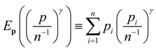 .
.