Network Coding for Line Networks with Broadcast Channels

Abstract

An achievable rate region for line networks with edge and node capacity constraints and broadcast channels (BCs) is derived. The region is shown to be the capacity region if the BCs are orthogonal, deterministic, physically degraded, or packet erasure with one-bit feedback. If the BCs are physically degraded with additive Gaussian noise then independent Gaussian inputs achieve capacity.

1. Introduction

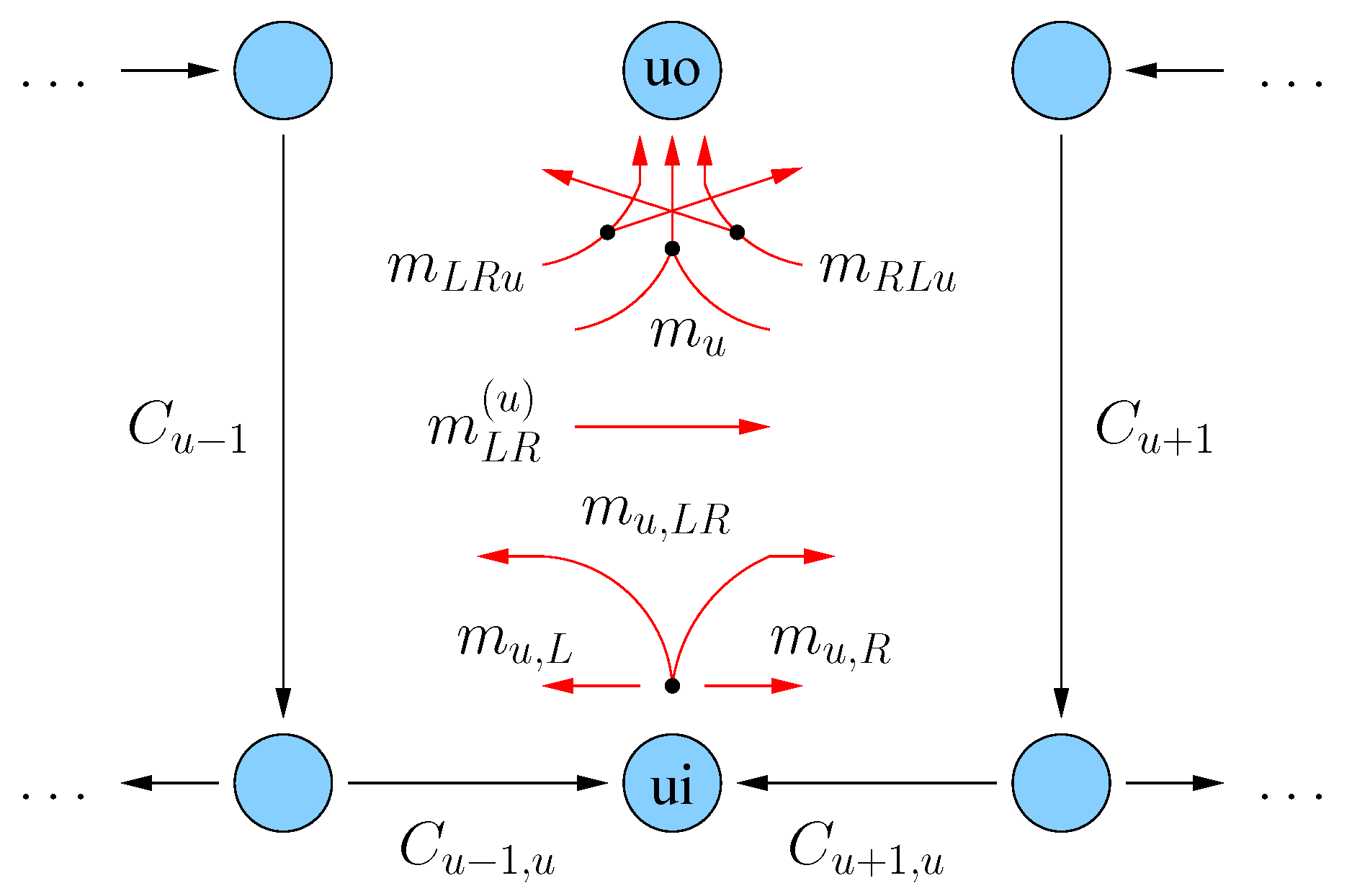
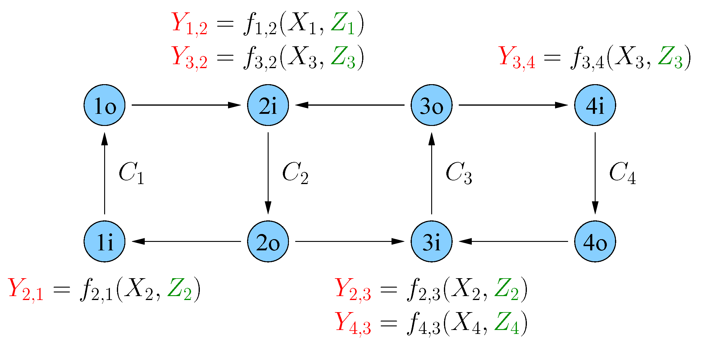
Consider a line network with edge and node capacity constraints as shown in Figure 1. “Supernode” u, $u=1,2,3,4$, consists of two nodes $ui,uo$ where the “i” represents “input” and “o” represents “output”. More generally, for N supernodes $\mathcal{V}=\{1,2,\dots ,N\}$ we have $2N$ nodes

$$\begin{array}{c}\hfill {\mathcal{V}}_{io}=\{1i,1o,2i,2o,\dots ,Ni,No\}\end{array}$$

(1)

and $2(N-1)+N$ directed edges

$$\begin{array}{cc}\hfill {\mathcal{E}}_{io}& =\left\{\right(1o,2i),(2o,3i),\dots ,((N-1)o,Ni\}\hfill \end{array}$$

$$\begin{array}{cc}& \cup \left\{\right(No,(N-1)i),\dots ,(3o,2i),(2o,1i\}\hfill \end{array}$$

$$\begin{array}{cc}& \cup \left\{\right(1i,1o),(2i,2o),\dots ,(Ni,No\left)\right\}\hfill \end{array}$$

(2)

Every edge $(a,b)$ is labeled with a capacity constraint $C_{(a,b)}$ and for simplicity we write $C_{(ui,uo)}$ as $C_u$.

Figure 1. A line network with edge and node capacity constraints.

Let

$$\begin{array}{c}\hfill u\to \mathcal{D}\left(u\right)=\left\{v\right(1),v(2),\dots ,v(L\left)\right\}\end{array}$$

(3)

denote a multicast traffic session, where $u,v\left(1\right),\dots ,v\left(L\right)$ are supernodes. The meaning is that a source message is available at supernode u and is destined for supernodes in the set $\mathcal{D}\left(u\right)$. Since u takes on N values and $\mathcal{D}\left(u\right)$ can take on $2^{N-1}-1$ values, there are up to $N(2^{N-1}-1)$ multicast sessions. We associate sources with input nodes $ui$ and sinks with output nodes $uo$. Such line networks are special cases of discrete memoryless networks (DMNs) and we use the capacity definition from [1] (Section III.D). The capacity region was recently established in [2]. A binary linear network code achieves capacity and progressive d-separating edge-cut (PdE) bounds [3] provide the converse.

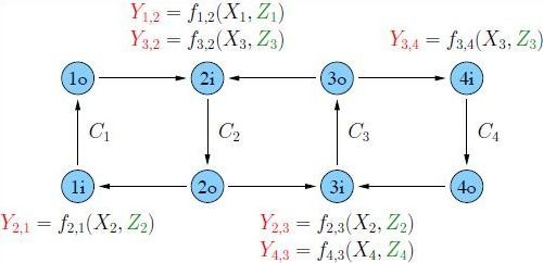
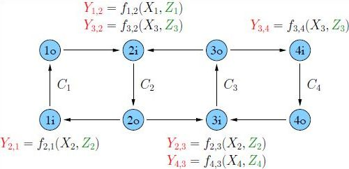
The goal of this work is to extend results from [2] to wireless line networks by using insights from two-way relaying [4], broadcasting with cooperation [5], and broadcasting with side-information [6]. The model is shown in Figure 2 where the difference to Figure 1 is that node $uo$ transmits over a two-receiver broadcast channel (BC) $P(y_{u-1},y_{u+1}|x_u)$ to nodes $(u-1)i$ and $(u+1)i$ (see [7]). The channel outputs at node $ui$ are

$$\begin{array}{cc}& Y_{u-1,u}=f_{u-1,u}(X_{u-1},Z_{u-1})\hfill \end{array}$$

(4)

$$\begin{array}{cc}& Y_{u+1,u}=f_{u+1,u}(X_{u+1},Z_{u+1})\hfill \end{array}$$

(5)

for some functions $f_{u-1,u}(·)$ and $f_{u+1,u}(·)$, and where the $Z_u$, $u=1,2,\dots ,N$, are statistically independent. We permit the noise random variables $Z_u$ to be common to $Y_{u,u-1}$ and $Y_{u,u+1}$ for generality. The edges $(ui,uo)$ are the usual links with capacity $C_u$. Such line networks are again special cases DMNs and we use the capacity definition from [1] (Section III.D).

Figure 2. A line network with broadcasting and node capacity constraints.

The paper is organized as follows. Section 2 reviews the capacity region for line networks derived in [2]. Section 3 gives our main result: an achievable rate region for line networks with BCs. Section 4 shows that this region is the capacity region for orthogonal, deterministic, and physically degraded BCs, and packet erasure BCs with feedback. We further show that for physically degraded Gaussian BCs the best input distributions are Gaussian. Section 5 relates our work to recent work on relaying and concludes the paper.

2. Review of Wireline Capacity

We review the main result from [2]. Let $m(u\to \mathcal{D}(u\left)\right)$ and $R(u\to \mathcal{D}(u\left)\right)$ denote the message bits and rate, respectively, of traffic session $u\to \mathcal{D}\left(u\right)$. We collect the bits going through supernode u into the following 8 sets:

$$\begin{array}{cc}\hfill m_{LR}^{\left(u\right)}& =\left\{m\right(i\to \mathcal{D}\left(i\right)):1\le i\le u-1,\mathcal{D}(i)\cap \{u+1,\dots ,N\}\ne \varnothing ,u\notin \mathcal{D}(i\left)\right\}\hfill \end{array}$$

(6)

$$\begin{array}{cc}\hfill m_{RL}^{\left(u\right)}& =\left\{m\right(i\to \mathcal{D}\left(i\right)):u+1\le i\le N,\mathcal{D}(i)\cap \{1,\dots ,u-1\}\ne \varnothing ,u\notin \mathcal{D}(i\left)\right\}\hfill \end{array}$$

(7)

$$\begin{array}{cc}\hfill m_{LRu}& =\left\{m\right(i\to \mathcal{D}\left(i\right)):1\le i\le u-1,\mathcal{D}(i)\cap \{u+1,\dots ,N\}\ne \varnothing ,u\in \mathcal{D}(i\left)\right\}\hfill \end{array}$$

(8)

$$\begin{array}{cc}\hfill m_{RLu}& =\left\{m\right(i\to \mathcal{D}\left(i\right)):u+1\le i\le N,\mathcal{D}(i)\cap \{1,\dots ,u-1\}\ne \varnothing ,u\in \mathcal{D}(i\left)\right\}\hfill \end{array}$$

(9)

$$\begin{array}{cc}\hfill m_u& =\left\{m\right(i\to \mathcal{D}\left(i\right)):1\le i\le u-1,\mathcal{D}(i)\cap \{u+1,\dots ,N\}=\varnothing ,u\in \mathcal{D}(i\left)\right\}\hfill \end{array}$$

$$\begin{array}{cc}& \bigcup \left\{m\right(i\to \mathcal{D}\left(i\right)):u+1\le i\le N,\mathcal{D}(i)\cap \{1,\dots ,u-1\}=\varnothing ,u\in \mathcal{D}(i\left)\right\}\hfill \end{array}$$

(10)

$$\begin{array}{cc}\hfill m_{u,LR}& =\left\{m\right(u\to \mathcal{D}\left(u\right)):\mathcal{D}(u)\cap \{1,\dots ,u-1\}\ne \varnothing \},\mathcal{D}\left(u\right)\cap \{u+1,\dots ,n\}\ne \varnothing \left\}\right\}\hfill \end{array}$$

(11)

$$\begin{array}{cc}\hfill m_{u,R}& =\left\{m\right(u\to \mathcal{D}\left(u\right)):\mathcal{D}(u)\cap \{1,\dots ,u-1\}=\varnothing \},\mathcal{D}\left(u\right)\cap \{u+1,\dots ,n\}\ne \varnothing \left\}\right\}\hfill \end{array}$$

(12)

$$\begin{array}{cc}\hfill m_{u,L}& =\left\{m\right(u\to \mathcal{D}\left(u\right)):\mathcal{D}(u)\cap \{1,\dots ,u-1\}\ne \varnothing \},\mathcal{D}\left(u\right)\cap \{u+1,\dots ,n\}=\varnothing \left\}\right\}\hfill \end{array}$$

(13)

The idea is that

• $m_{LR}^{\left(u\right)}$ and $m_{RL}^{\left(u\right)}$ represent traffic flowing from left-to-right and right-to-left, respectively, through supernode u without being required at supernode u;
• $m_{LRu}$, $m_{RLu}$ represent traffic flowing from left-to-right and right-to-left, respectively, through supernode u but required at supernode u also;
• $m_u$ represents traffic from the left and right, respectively, and destined for supernode u but not destined for any nodes on the right and left (so this traffic “stops" at supernode u on its way from the left or right);
• $m_{u,LR}$, $m_{u,R}$, and $m_{u,L}$ represent traffic originating at supernode u and destined for nodes on both the left and right, right only, and left only, respectively.

The non-negative message rates are denoted $R_{LR}^{\left(u\right)}$, $R_{RL}^{\left(u\right)}$, $R_{LRu}$, $R_{RLu}$, $R_u$, $R_{u,LR}$, $R_{u,R}$, and $R_{u,L}$.

Theorem 1 (Theorem 1 in [2]) 

The capacity region of a line network with supernodes $u=1,2,\dots ,N$ is specified by the inequalities

$$\begin{array}{cc}& max(R_{LR}^{\left(u\right)},R_{RL}^{\left(u\right)})+R_{LRu}+R_{RLu}+R_u+R_{u,LR}+R_{u,R}+R_{u,L}\le C_u\hfill \end{array}$$

(14)

$$\begin{array}{cc}& R_{RL}^{\left(u\right)}+R_{RLu}+R_{u,LR}+R_{u,L}\le C_{u,u-1}\hfill \end{array}$$

(15)

$$\begin{array}{cc}& R_{LR}^{\left(u\right)}+R_{LRu}+R_{u,LR}+R_{u,R}\le C_{u,u+1}\hfill \end{array}$$

(16)

Remark 1 The converse in [2] follows by PdE arguments [3] and achievability follows by using rate-splitting, routing, copying, and “butterfly” binary linear network coding. We review both the PdE bound and the coding method after Examples 1 and 2 below.

Remark 2 Inequalities (15) and (16) are classic cut bounds [8] (Section 14.10). If we have no node constraints ($C_u=\infty$) then (15) and (16) are routing bounds, so routing is optimal for this case (see [9]).

Example 1 Consider $N=3$ for which we have 9 possible multicast sessions. The network is as in Figure 1 but where the nodes $4i$ and $4o$ are removed, as well as the edges touching them. For supernode $u=1$ we collect 7 of these sessions into 2 sets as follows. (We abuse notation and write $u\to \left\{v\right\}$ as $u\to v$.)

$$\begin{array}{cc}\hfill m_1& :2\to 1,2\to \{1,3\},3\to 1,3\to \{1,2\}\hfill \end{array}$$

(17)

$$\begin{array}{cc}\hfill m_{1,R}& :1\to 2,1\to 3,1\to \{2,3\}\hfill \end{array}$$

(18)

Sessions $2\to 3$ and $3\to 2$ are missing from (17) and (18) because they do not involve supernode 1. Similarly, for supernode 2 we collect the 9 sessions into 8 sets:

$$\begin{array}{cc}& m_{LR}^{\left(2\right)}:1\to 3,m_{RL}^{\left(2\right)}:3\to 1,m_{LR2}:1\to \{2,3\},m_{RL2}:3\to \{1,2\}\hfill \end{array}$$

(19)

$$\begin{array}{cc}& m_2:1\to 2,3\to 2,m_{2,LR}:2\to \{1,3\},m_{2,R}:2\to 3,m_{2,L}:2\to 1\hfill \end{array}$$

(20)

Finally, for supernode 3 we have the 2 sets

$$\begin{array}{cc}\hfill m_3& :1\to 3,1\to \{2,3\},2\to 3,2\to \{1,3\}\hfill \end{array}$$

(21)

$$\begin{array}{cc}\hfill m_{3,L}& :3\to 1,3\to 2,3\to \{1,2\}\hfill \end{array}$$

(22)

The inequalities of Theorem 1 are

$$\begin{array}{cc}& u=1:\left\{\begin{array}{c}{R}_1+R_{1,R}\le C_1\hfill \\ R_{1,R}\le C_{1,2}\hfill \end{array}\right.\hfill \end{array}$$

(23)

$$\begin{array}{cc}& u=2:\left\{\begin{array}{c}max(R_{LR}^{\left(2\right)},R_{RL}^{\left(2\right)})+R_{LR2}+R_{RL2}+R_2+R_{2,LR}+R_{2,R}+R_{2,L}\le C_2\hfill \\ R_{RL}^{\left(2\right)}+R_{RL2}+R_{2,LR}+R_{2,L}\le C_{2,1}\hfill \\ R_{LR}^{\left(2\right)}+R_{LR2}+R_{2,LR}+R_{2,R}\le C_{2,3}\hfill \end{array}\right.\hfill \end{array}$$

(24)

$$\begin{array}{cc}& u=3:\left\{\begin{array}{c}{R}_3+R_{3,L}\le C_3\hfill \\ R_{3,L}\le C_{3,2}\hfill \end{array}\right.\hfill \end{array}$$

(25)

We discuss the 7 inequalities (23)–(25) in more detail. Consider first the converse. We write a classic cut as $(\mathcal{S},{\mathcal{S}}^c)$, where $\mathcal{S}$ is the set of nodes on one side of the cut and ${\mathcal{S}}^c$ is the set of nodes on the other side of the cut. The inequalities with the edge capacities $C_{1,2}$, $C_{2,1}$, $C_{2,3}$, $C_{3,2}$ are classic cut bounds. For example, the cut $(\mathcal{S},{\mathcal{S}}^c)=(\{1i,1o\},\{2i,2o,3i,3o\})$ gives the bound $R_{1,R}\le C_{1,2}$.

The inequalities with the “node" capacities $C_1$, $C_2$, $C_3$ in (23)–(25) are not classic cut bounds. To see this, consider the bound $R_1+R_{1,R}\le C_1$. A classic cut bound would require us to choose $\{1o,2o,3o\}\subseteq {\mathcal{S}}^c$ because $m_1$ and $m_{1,R}$ generally include messages with positive rates for all supernodes. But then the only way to isolate the edge $(1i,1o)$ is to choose $\mathcal{S}=\left\{1i\right\}$ which gives the too-weak bound $R_{1,R}\le C_1$.

We require a stronger method and use PdE bounds. We use the notation in [3]: ${\mathcal{E}}_d$ is the edge cut, ${\mathcal{S}}_d$ is the set of sources whose sum-rate we bound, $\pi (·)$ is the permutation that defines the order in which we test the sources. Consider the edge cut ${\mathcal{E}}_d=\left\{(1i,1o)\right\}$, the source set ${\mathcal{S}}_d$ with the traffic sessions (17) and (18), and any permutation $\pi (·)$ for which the sessions (17) appear before the sessions (18). After removing edge $(1i,1o)$ the PdE algorithm removes edge $(1o,2i)$ because node $1o$ has no incoming edges. We next test if the sessions (17) are disconnected from one of their destinations; indeed they are because one of these destinations is node $1o$. The PdE algorithm now removes the remaining edges in the graph because the nodes $2i,2o,3i,3o$ are not the sources of messages in (18). As a result, the remaining sessions (18) are disconnected from their destinations and the PdE bound gives $R_1+R_{1,R}\le C_1$. The bound on $C_3$ follows similarly. The bound on $C_2$ is more subtle and we develop it in a more general context below (see the text after Example 2).

For achievability, note that all 7 inequalities are routing bounds except for the bound on $C_2$ in (24). To approach this bound, we use a classic method and XOR the bits in sessions $1\to 3$ and $3\to 1$ before sending them through edge $(2i,2o)$. More precisely, we combine $m(1\to 3)$ and $m(3\to 1)$ to form

$$\begin{array}{c}\hfill m(1\to 3)\oplus m(3\to 1)\end{array}$$

(26)

by which we mean the bits formed when the smaller-rate message bits are XORed with a corresponding number of bits of the larger-rate message. The remaining larger-rate message bits are appended so that $m(1\to 3)\oplus m(3\to 1)$ has rate $max\left(R\right(1\to 3),R(3\to 1\left)\right)$. The message (26) is sent to node $2o$ together with the remaining messages received at node $2i$. We must thus satisfy the bound on $C_2$ in (24).

For the routing bounds there are two subtleties. First, node $2o$ forwards to the left the uncoded bits $m(3\to \{1,2\left\}\right)$, $m(2\to \{1,3\left\}\right)$, and $m(2\to 1)$. However, it must treat $m(1\to 3)\oplus m(3\to 1)$ specially because it cannot necessarily determine $m(3\to 1)$ and $m(1\to 3)$. But if $R(1\to 3)>R(3\to 1)$ then node $2o$ can remove the appended bits in (26) and communicate $m(3\to 1)$ to node $1i$ at rate $R(3\to 1)$, rather than $max\left(R\right(1\to 3),R(3\to 1\left)\right)$. If $R(1\to 3)\le R(3\to 1)$ then no bits should be removed and node $2o$ again communicates $m(3\to 1)$ to node $1i$ at rate $R(3\to 1)$. The bits node $2o$ forwards to the right are treated similarly. In summary, the rates for messages $m(3\to 1)$ and $m(1\to 3)$ on edges $(2o,1i)$ and $(2o,3i)$, respectively, are simply the classic routing rates.

The second routing subtlety is more straightforward: after node $1i$ receives the XORed bits, it can recover $m(3\to 1)$ by subtracting the bits $m(1\to 3)$ that it knows. Finally, node $1i$ transmits $m(3\to 1)$ to node $1o$. Node $3i$ operates similarly.

Example 2 Consider Figure 1 with $N=4$ for which there are 28 possible multicast sessions. For supernode 1 we collect 19 of these sessions into 2 sets as follows.

$$\begin{array}{cc}\hfill m_1& :2\to 1,2\to \{1,3\},2\to \{1,4\},2\to \{1,3,4\},\hfill \end{array}$$

$$\begin{array}{cc}& 3\to 1,3\to \{1,2\},3\to \{1,4\},3\to \{1,2,4\},\hfill \end{array}$$

$$\begin{array}{cc}& 4\to 1,4\to \{1,2\},4\to \{1,3\},4\to \{1,2,3\}\hfill \end{array}$$

(27)

$$\begin{array}{cc}\hfill m_{1,R}& :1\to 2,1\to 3,1\to 4,\hfill \end{array}$$

$$\begin{array}{cc}& 1\to \{2,3\},1\to \{2,4\},1\to \{3,4\},\hfill \end{array}$$

$$\begin{array}{cc}& 1\to \{2,3,4\}\hfill \end{array}$$

(28)

The 9 sessions not involving supernode 1 are missing. The rate bounds for supernode 1 are given by (14)–(16) with $u=1$. The messages and rate bounds for supernode 4 are similar.

Similarly, for supernode 2 we collect 26 of 28 sessions into 8 sets as follows.

$$\begin{array}{cc}\hfill m_{LR}^{\left(2\right)}& :1\to 3,1\to 4,1\to \{3,4\}\hfill \end{array}$$

(29)

$$\begin{array}{cc}\hfill m_{RL}^{\left(2\right)}& :3\to 1,3\to \{1,4\},4\to 1,4\to \{1,3\}\hfill \end{array}$$

(30)

$$\begin{array}{cc}\hfill m_{LR2}& :1\to \{2,3\},1\to \{2,4\},1\to \{2,3,4\}\hfill \end{array}$$

(31)

$$\begin{array}{cc}\hfill m_{RL2}& :3\to \{1,2\},3\to \{1,2,4\},4\to \{1,2\},4\to \{1,2,3\}\hfill \end{array}$$

(32)

$$\begin{array}{cc}\hfill m_2& :1\to 2,3\to 2,3\to \{2,4\},4\to 2,4\to \{2,3\}\hfill \end{array}$$

(33)

$$\begin{array}{cc}\hfill m_{2,LR}& :2\to \{1,3\},2\to \{1,4\},2\to \{1,3,4\}\hfill \end{array}$$

(34)

$$\begin{array}{cc}\hfill m_{2,R}& :2\to 3,2\to 4,2\to \{3,4\}\hfill \end{array}$$

(35)

$$\begin{array}{cc}\hfill m_{2,L}& :2\to 1\hfill \end{array}$$

(36)

Sessions $3\to 4$ and $4\to 3$ are missing. The rate bounds for supernode 2 are given by (14)–(16) with $u=2$. The messages and rate bounds for supernode 3 are similar.

The converse and coding method for $N>3$ are entirely similar to the case $N=3$. However, we have not yet developed the PdE bound for $N=3$ and edge cut ${\mathcal{E}}_d=\left\{(2i,2o)\right\}$. We do this now but in the more general context of $N\ge 2$ and ${\mathcal{E}}_d=\left\{(ui,uo)\right\}$ for any u.

So consider the PdE bound with ${\mathcal{E}}_d=\left\{(ui,uo)\right\}$ and ${\mathcal{S}}_d$ having all the traffic sessions (6)–(13) except for (7). We choose $\pi (·)$ so that the sessions (8)–(10) appear first, the sessions (6) and (11)–(12) appear second, and the sessions (13) appear last. The PdE algorithm performs the following steps.

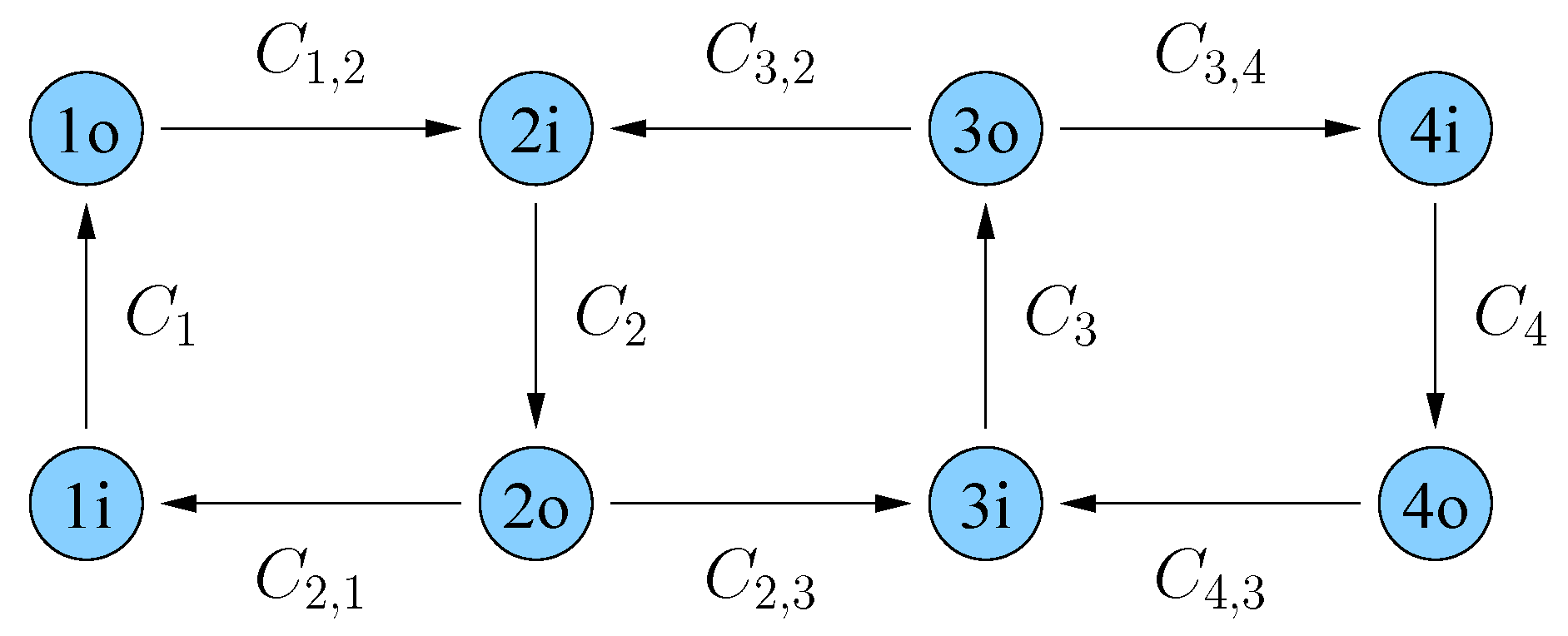
• Remove $(ui,uo)$ and then remove $(uo,(u-1\left)i\right)$ and $(uo,(u+1\left)i\right)$ because node $uo$ has no incoming edges. The resulting graph at supernode u is shown in Figure 3.
• Test if the sessions (8)–(10) (sessions $m_{LRu}$, $m_{RLu}$, $m_u$) are disconnected from one of their destinations, which they are because one of these destinations is node $uo$.
• Remove all edges to the right of supernode u because the nodes to the right are not the sources of the remaining sessions (6), (11)–(13) (sessions $m_{LR}^{\left(u\right)}$, $m_{u,LR}$, $m_{u,R}$, and $m_{u,L}$).
• Test if the sessions (6), (11) and (12) (sessions $m_{LR}^{\left(u\right)}$, $m_{u,LR}$, $m_{u,R}$) are disconnected from one of their destinations, which they are because one of these destinations is to the right of supernode u.
• Remove all edges to the left of supernode u because the nodes to the left are not the sources of the sessions (13) (sessions $m_{u,L}$).
• Test if the sessions (13) are disconnected from one of their destinations, which they are.

Since the algorithm completes successfully, the PdE bound (almost) gives inequality (14), but with $R_{LR}^{\left(u\right)}$ replacing $max(R_{LR}^{\left(u\right)},R_{RL}^{\left(u\right)})$. The other inequality, i.e., the one with $R_{RL}^{\left(u\right)}$ replacing $max(R_{LR}^{\left(u\right)},R_{RL}^{\left(u\right)})$ follows by choosing ${\mathcal{S}}_d$ with all the traffic sessions (6)–(13) except for (6), and by modifying $\pi (·)$ so that the edges to the left of supernode u are removed first, and then the edges to the right.

Figure 3. Network at supernode u after the PdE bound has removed the edges $(ui,uo)$, $(uo,(u-1\left)i\right)$, and $(uo,(u+1\left)i\right)$. The session messages are tested in the order: $m_{LRu}$, $m_{RLu}$, $m_u$, then $m_{LR}^{\left(u\right)}$, $m_{u,LR}$, $m_{u,R}$, and finally $m_{u,L}$.

3. Achievable Rates with Broadcast

We separate channel and network coding, which sounds simple enough. However, every BC receiver has side information about some of the messages being transmitted, so we will need the methods of [6]. We further use the theory in [5] to describe our achievable rate region.

We begin by having each node $ui$ combine $m_{LR}^{\left(u\right)}$ and $m_{RL}^{\left(u\right)}$ into the message

$$\begin{array}{c}\hfill m_{LR}^{\left(u\right)}\oplus m_{RL}^{\left(u\right)}\end{array}$$

(37)

by which we mean the same operation as in (26): the smaller-rate message bits are XORed with a corresponding number of bits of the larger-rate message. The remaining larger-rate message bits are appended so that $m_{LR}^{\left(u\right)}\oplus m_{RL}^{\left(u\right)}$ has rate $max(R_{LR}^{\left(u\right)},R_{RL}^{\left(u\right)})$. The message (37) is sent to node $uo$ together with the remaining messages received at node $ui$. As a result, we must satisfy the bound (14).

The bits arriving at node $uo$ are (37) and (8)–(13). Bits $m_u$ are removed at node $uo$ since this node is their final destination. The bits (37) and (8)–(9) and (11) must be broadcast to both nodes $(u-1)i$ and $(u+1)i$. The remaining bits $m_{u,R}$ and $m_{u,L}$ are destined (or dedicated) for the right and left only, respectively. However, we know from information theory for broadcast channels [7] that it can help to broadcast parts of these dedicated messages to both receivers. So we split $m_{u,R}$ and $m_{u,L}$ into two parts each, namely the respective $(m_{u,R}^{\prime },m_{u,R}^{\prime \prime })$ and $(m_{u,L}^{\prime },m_{u,L}^{\prime \prime })$ where $m_{u,R}^{\prime }$ and $m_{u,L}^{\prime }$ are broadcast to both nodes $(u-1)i$ and $(u+1)i$. The rates of $m_{u,R}^{\prime }$ and $m_{u,R}^{\prime \prime }$ are the respective $R_{u,R}^{\prime }$ and $R_{u,R}^{\prime \prime }$, and similarly for $R_{u,L}^{\prime }$ and $R_{u,L}^{\prime \prime }$. We choose a joint distribution $P_{S_u{T}_u{W}_u{X}_u}(·)$ and generate a codebook of size

$$2^{n\left(max\left(R_{LR}^{\left(u\right)},R_{RL}^{\left(u\right)}\right)+R_{LRu}+R_{RLu}+R_{u,LR}+R_{u,R}^{\prime }+R_{u,L}^{\prime }\right)}$$

with length-n codewords

$${\underline{w}}_u\left(m_{LR}^{\left(u\right)}\oplus m_{RL}^{\left(u\right)},m_{LRu},m_{RLu},m_{u,LR},m_{u,R}^{\prime },m_{u,L}^{\prime }\right)$$

by choosing every letter of every codeword independently using $P_{W_u}(·)$.

We next choose “binning" rates $R_{T_u}$ and $R_{S_u}$. For every ${\underline{w}}_u$, we choose $2^{n(R_{u,R}^{\prime \prime }+R_{T_u})}$ length-n codewords ${\underline{t}}_u$ by choosing the ith letter $t_{u,i}$ of ${\underline{t}}_u$ via the distribution $P_{T_u|W_u}(·|w_{u,i})$ where $w_{u,i}$ is the ith letter of ${\underline{w}}_u$. We label ${\underline{t}}_u$ with the arguments of ${\underline{w}}_u$, $m_{u,R}^{\prime \prime }$, and a “bin” index from $\{1,2,\dots ,2^{n{R}_{T_u}}\}$. Similarly, for every ${\underline{w}}_u$ we generate $2^{n(R_{u,L}^{\prime \prime }+R_{S_u})}$ length-n codewords ${\underline{s}}_u$ generated via $P_{S_u|W_u}(·)$ and label ${\underline{s}}_u$ with the arguments of ${\underline{w}}_u$, $m_{u,L}^{\prime \prime }$, and a “bin” index from $\{1,2,\dots ,2^{n{R}_{S_u}}\}$.

Next, the encoder tries to find a pair of bin indices such that $({\underline{w}}_u,{\underline{t}}_u,{\underline{s}}_u)$ is jointly typical according to one’s favorite flavor of typicality. Using standard typicality arguments (see, e.g., [5]) a typical triple exists with high probability if n is large and

$$\begin{array}{c}\hfill R_{S_u}+R_{T_u}>I(S_u;T_u|W_u)\end{array}$$

(38)

Once this triple is found, we transmit a length-n signal ${\underline{x}}_u$ that is generated via $P_{X_u|S_u{T}_u{W}_u}(·|s_{u,i},t_{u,i},w_{u,i})$ for $i=1,2,\dots ,n$.

The receivers use joint typicality decoders to recover their messages. They further use their knowledge (or side-information) about some of the messages. The result is that decoding is reliable if n is large and if the following rate constraints are satisfied (see [5,6]):

$$\begin{array}{cc}& R_{u,L}^{\prime \prime }+R_{S_u}<I(S_u;Y_{u,u-1}|W_u)\hfill \end{array}$$

(39)

$$\begin{array}{cc}& R_{RL}^{\left(u\right)}+R_{RLu}+R_{u,LR}+R_{u,R}^{\prime }+R_{u,L}+R_{S_u}<I(S_u{W}_u;Y_{u,u-1})\hfill \end{array}$$

(40)

$$\begin{array}{cc}& R_{u,R}^{\prime \prime }+R_{T_u}<I(T_u;Y_{u,u+1}|W_u)\hfill \end{array}$$

(41)

$$\begin{array}{cc}& R_{LR}^{\left(u\right)}+R_{LRu}+R_{u,LR}+R_{u,R}+R_{u,L}^{\prime }+R_{T_u}<I(T_u{W}_u;Y_{u,u+1})\hfill \end{array}$$

(42)

Finally, we use Fourier–Motzkin elimination (see [5]) to remove $R_{S_u}$, $R_{T_u}$, $R_{u,L}^{\prime }$, $R_{u,R}^{\prime }$, $R_{u,L}^{\prime \prime }$, and $R_{u,R}^{\prime \prime }$ from the above expressions and obtain the following result.

Theorem 2 

An achievable rate region for a line network with broadcast channels is given by the bounds

$$\begin{array}{cc}& max(R_{LR}^{\left(u\right)},R_{RL}^{\left(u\right)})+R_{LRu}+R_{RLu}+R_u+R_{u,LR}+R_{u,R}+R_{u,L}\le C_u\hfill \end{array}$$

(43)

$$\begin{array}{cc}& R_{RL}^{\left(u\right)}+R_{RLu}+R_{u,LR}+R_{u,L}\le I(S_u{W}_u;Y_{u,u-1})\hfill \end{array}$$

(44)

$$\begin{array}{cc}& R_{LR}^{\left(u\right)}+R_{LRu}+R_{u,LR}+R_{u,R}\le I(T_u{W}_u;Y_{u,u+1})\hfill \end{array}$$

(45)

$$\begin{array}{cc}& R_{RL}^{\left(u\right)}+R_{RLu}+R_{u,LR}+R_{u,R}+R_{u,L}\le I(S_u{W}_u;Y_{u,u-1})+I(T_u;Y_{u,u+1}|W_u)-I(S_u;T_u|W_u)\hfill \end{array}$$

(46)

$$\begin{array}{cc}& R_{LR}^{\left(u\right)}+R_{LRu}+R_{u,LR}+R_{u,R}+R_{u,L}\le I(T_u{W}_u;Y_{u,u+1})+I(S_u;Y_{u,u-1}|W_u)-I(S_u;T_u|W_u)\hfill \end{array}$$

(47)

$$\begin{array}{cc}& R_{LR}^{\left(u\right)}+R_{RL}^{\left(u\right)}+R_{LRu}+R_{RLu}+2R_{u,LR}+R_{u,R}+R_{u,L}\hfill \end{array}$$

$$\begin{array}{cc}& \le I(S_u{W}_u;Y_{u,u-1})+I(T_u{W}_u;Y_{u,u+1})-I(S_u;T_u|W_u)\hfill \end{array}$$

(48)

for any choice of $P(s_u,t_u,w_u,x_u)$ and for all u, and where $S_u{T}_u{W}_u-X_u-Y_{u,u-1}{Y}_{u,u+1}$ forms a Markov chain for all u.

Remark 3 The bound (43) is the same as (14).

Remark 4 The bounds (44)–(48) are similar to the bounds of [5, Theorem 5]. A few rates are “missing” because nodes $(u-1)i$ and $(u+1)i$ know $(m_{LR}^{\left(u\right)},m_{LRu})$ and $(m_{RL}^{\left(u\right)},m_{RLu})$, respectively, when decoding.

Example 3 Consider $N=3$ for which we have the sessions (17)–(22). The inequalities of Theorem 2 are

$$\begin{array}{cc}& u=1:\left\{\begin{array}{c}{R}_1+R_{1,R}\le C_1\hfill \\ R_{1,R}\le I(T_1;Y_{1,2}|W_1)-I(S_1;T_1|W_1)\hfill \end{array}\right.\hfill \end{array}$$

(49)

$$\begin{array}{cc}& u=2:\left\{\begin{array}{c}max(R_{LR}^{\left(2\right)},R_{RL}^{\left(2\right)})+R_{LR2}+R_{RL2}+R_2+R_{2,LR}+R_{2,R}+R_{2,L}\le C_2\hfill \\ Thefiveinequalities\text{(44)–(48)}withu=2\hfill \end{array}\right.\hfill \end{array}$$

(50)

$$\begin{array}{cc}& u=3:\left\{\begin{array}{c}{R}_3+R_{3,L}\le C_3\hfill \\ R_{3,L}\le I(S_3;Y_{3,2}|W_3)-I(S_3;T_3|W_3)\hfill \end{array}\right.\hfill \end{array}$$

(51)

Observe that the channels from node $1o$ to node $2i$, and node $3o$ to node $2i$, are memoryless channels with capacities $C_{1,2}$ and $C_{3,2}$, respectively. In fact, from (49) and (51) it is easy to see that we may as well choose $W_1$, $S_1$, $W_3$, and $T_3$ as constants. Moreover, we should choose $T_1=X_1$ and $S_3=X_3$, and then choose the input distributions so that $I(X_1;Y_{1,2})=C_{1,2}$ and $I(X_3;Y_{3,2})=C_{3,2}$. The inequalities (44)–(48) at node $u=2$ correspond to Marton’s region [10] (Section 7.8) for broadcast channels including a common rate. We will see in the next section that if we specialize to the model of [2] then only the bounds (43)–(45) remain at node 2 because the bounds (46)–(48) are redundant.

4. Special Channels

4.1. Orthogonal Channels

A BC $P_{Y_1{Y}_2|X}$ is orthogonal if $X=(X_1,X_2)$ and $P_{Y_1{Y}_2|X}=P_{Y_1|X_1}{P}_{Y_2|X_2}$ (see [8] (p. 419)). In fact, if all BCs in Figure 2 are orthogonal then the model reduces to that of Figure 1 so hopefully we recover Theorem 1 from Theorem 2.

Let $X_u=(X_{u,u-1},X_{u,u+1})$ and $Y_u=(Y_{u-1,u},Y_{u+1,u})$. Suppose $C_{u,u-1}$ and $C_{u,u+1}$ are the respective capacities of the memoryless channels $P_{Y_{u,u-1}|X_{u,u-1}}$ and $P_{Y_{u,u+1}|X_{u,u+1}}$. We choose $S_u=X_{u,u-1}$, $T_u=X_{u,u+1}$, $W_u=0$, and $X_{u,u-1},X_{u,u+1}$ to be independent and capacity-achieving. Inequalities (44)–(48) reduce to

$$\begin{array}{cc}& R_{RL}^{\left(u\right)}+R_{RLu}+R_{u,LR}+R_{u,L}\le C_{u,u-1}\hfill \end{array}$$

(52)

$$\begin{array}{cc}& R_{LR}^{\left(u\right)}+R_{LRu}+R_{u,LR}+R_{u,R}\le C_{u,u+1}\hfill \end{array}$$

(53)

The region of Theorem 1 is therefore achievable. The converse follows by using the same steps as in the converse of Theorem 1.

4.2. Deterministic Channels

A BC $P_{Y_1{Y}_2|X}$ is deterministic if $Y_1=f_1\left(X\right)$ and $Y_2=f_2\left(X\right)$ for some functions $f_1(·)$ and $f_2(·)$. We show that Theorem 2 gives the capacity region if all BCs in Figure 2 are deterministic.

Theorem 3 

The capacity region of a line network with deterministic BCs is the union over all $P(w_u,x_u)$, $u=1,2,\dots ,N$, of the (non-negative) rates satisfying

$$\begin{array}{cc}& max(R_{LR}^{\left(u\right)},R_{RL}^{\left(u\right)})+R_{LRu}+R_{RLu}+R_u+R_{u,LR}+R_{u,R}+R_{u,L}\le C_u\hfill \end{array}$$

(54)

$$\begin{array}{cc}& R_{RL}^{\left(u\right)}+R_{RLu}+R_{u,LR}+R_{u,L}\le H\left(Y_{u,u-1}\right)\hfill \end{array}$$

(55)

$$\begin{array}{cc}& R_{LR}^{\left(u\right)}+R_{LRu}+R_{u,LR}+R_{u,R}\le H\left(Y_{u,u+1}\right)\hfill \end{array}$$

(56)

$$\begin{array}{cc}& R_{RL}^{\left(u\right)}+R_{RLu}+R_{u,LR}+R_{u,R}+R_{u,L}\le I(W_u;Y_{u,u-1})+H\left(Y_{u,u-1}{Y}_{u,u+1}\right|W_u)\hfill \end{array}$$

(57)

$$\begin{array}{cc}& R_{LR}^{\left(u\right)}+R_{LRu}+R_{u,LR}+R_{u,R}+R_{u,L}\le I(W_u;Y_{u,u+1})+H\left(Y_{u,u-1}{Y}_{u,u+1}\right|W_u)\hfill \end{array}$$

(58)

$$\begin{array}{cc}& R_{LR}^{\left(u\right)}+R_{RL}^{\left(u\right)}+R_{LRu}+R_{RLu}+2R_{u,LR}+R_{u,R}+R_{u,L}\hfill \end{array}$$

$$\begin{array}{cc}& \le I(W_u;Y_{u,u-1})+I(W_u;Y_{u,u+1})+H\left(Y_{u,u-1}{Y}_{u,u+1}\right|W_u)\hfill \end{array}$$

(59)

Proof. 

Achievability follows by Theorem 2 with $S_u=Y_{u,u-1}$ and $T_u=Y_{u,u+1}$. For the converse, the constraint (54) is the PdE bound of [11] (Section III.A). The bounds (55) and (56) are cut bounds. For the remaining steps, let ${\mathcal{S}}^c$ be the complement of $\mathcal{S}$ in $\mathcal{V}$. We define

$$\begin{array}{c}\hfill Y_{\mathcal{S},\mathcal{T}}=\{Y_{u,v}:u\in \mathcal{S},v\in \mathcal{T}\}\end{array}$$

(60)

Let $M_{u,L}$ be the random message corresponding to $m_{u,L}$, and similarly for the other messages. The messages are independent and have entropy equal to n times their rate, where n is the number of times we use each BC. Let $M\left(\mathcal{S}\right)$ be the set of messages originating at supernodes in $\mathcal{S}$. Let $M_{u,L}^c$ to be the set of all network messages except for $M_{u,L}$, and similarly for other messages. We use the notation

$$\begin{array}{cc}& Y_{u,u-1}^{i-1}=Y_{u,u-1,1},Y_{u,u-1,2},\dots ,Y_{u,u-1,i-1}\hfill \\ & {\tilde{W}}_{u,i}={\left(M_{u,L}{M}_{u,R}\right)}^c{Y}_{u,u-1}^{i-1}{Y}_{u,u+1}^{i-1}\hfill \end{array}$$

For the following, let $\mathcal{S}=\{u,u+1,\dots ,N\}$ and $\tilde{\mathcal{S}}=\{1,2,\dots ,u\}$. We bound

$$\begin{array}{cc}\hfill I\left(M_{RL}^{\left(u\right)}{M}_{RLu}{M}_{u,LR};Y_{\mathcal{S},{\mathcal{S}}^c}^{n}M\left({\mathcal{S}}^c\right)\right)& =I\left(M_{RL}^{\left(u\right)}{M}_{RLu}{M}_{u,LR};Y_{u,u-1}^n|M\left({\mathcal{S}}^c\right)\right)\hfill \end{array}$$

$$\begin{array}{cc}& \stackrel{\left(a\right)}{\le }I\left({\left(M_{u,L}{M}_{u,R}\right)}^c;Y_{u,u-1}^n\right)\hfill \end{array}$$

$$\begin{array}{cc}& =\sum _{i=1}^{n}I\left({\left(M_{u,L}{M}_{u,R}\right)}^c;Y_{u,u-1,i}|Y_{u,u-1}^{i-1}\right)\hfill \end{array}$$

$$\begin{array}{cc}& \stackrel{\left(a\right)}{\le }\sum _{i=1}^{n}I\left({\tilde{W}}_{u,i};Y_{u,u-1,i}\right)\hfill \end{array}$$

$$\begin{array}{cc}& \stackrel{\left(b\right)}{=}nI\left({\tilde{W}}_{u,Q};Y_{u,u-1,Q}|Q\right)\hfill \end{array}$$

$$\begin{array}{cc}& \stackrel{\left(c\right)}{\le }nI\left(W_u;Y_{u,u-1}\right)\hfill \end{array}$$

(61)

where steps $\left(a\right)$ follow by $I(A;B|C)\le I(ACD;B)$, step $\left(b\right)$ follows by defining Q to be a time-sharing random variable that is uniform over $1,2,\dots ,n$, and $\left(c\right)$ follows by defining $Y_{u,u-1}=Y_{u,u-1,Q}$ and $W_u={\tilde{W}}_{u,Q}Q$. We similarly have

$$\begin{array}{cc}\hfill I\left(M_{LR}^{\left(u\right)}{M}_{LRu}{M}_{u,LR};Y_{\tilde{\mathcal{S}},{\tilde{\mathcal{S}}}^c}^{n}M\left({\tilde{\mathcal{S}}}^c\right)\right)& \le nI\left(W_u;Y_{u,u+1}\right)\hfill \end{array}$$

(62)

where $Y_{u,u+1}=Y_{u,u+1,Q}$. Note that our choices for $Y_{u,u-1}$ and $Y_{u,u+1}$ are appropriate for the cut bounds (55) and (56). Finally, we have

$$\begin{array}{cc}\hfill I\left(M_{u,L}{M}_{u,R};Y_{\left\{u\right\},\mathcal{V}}^n{\left(M_{u,L}{M}_{u,R}\right)}^c\right)& =I\left(M_{u,L}{M}_{u,R};Y_{u,u-1}^n{Y}_{u,u+1}^n|{\left(M_{u,L}{M}_{u,R}\right)}^c\right)\hfill \end{array}$$

$$\begin{array}{cc}& =\sum _{i=1}^{n}H\left(Y_{u,u-1,i}{Y}_{u,u+1,i}|{\tilde{W}}_{u,i}\right)\hfill \end{array}$$

$$\begin{array}{cc}& =nH\left(Y_{u,u-1}{Y}_{u,u+1}|W_u\right)\hfill \end{array}$$

(63)

Consider the bound (57). We have

$$\begin{array}{cc}& n(R_{RL}^{\left(u\right)}+R_{RLu}+R_{u,LR}+R_{u,R}+R_{u,L})\hfill \end{array}$$

$$\begin{array}{cc}& \stackrel{\left(a\right)}{\le }I\left(M_{RL}^{\left(u\right)}{M}_{RLu}{M}_{u,LR};Y_{\mathcal{S},{\mathcal{S}}^c}^{n}M\left({\mathcal{S}}^c\right)\right)+I\left(M_{u,L}{M}_{u,R};Y_{\left\{u\right\},\mathcal{V}}^n{\left(M_{u,L}{M}_{u,R}\right)}^c\right)\hfill \end{array}$$

$$\begin{array}{cc}& \stackrel{\left(b\right)}{\le }nI\left(W_u;Y_{u,u-1}\right)+nH\left(Y_{u,u-1}{Y}_{u,u+1}|W_u\right)\hfill \end{array}$$

(64)

where $\left(a\right)$ follows by Fano’s inequality [8] (p. 38) when the block error probability tends to zero, and $\left(b\right)$ follows by (61) and (63). This proves (57), and (58) follows in the same way.

Finally, for (59) we use Fano’s inequality to bound

$$\begin{array}{cc}& n(R_{LR}^{\left(u\right)}+R_{RL}^{\left(u\right)}+R_{LRu}+R_{RLu}+2R_{u,LR}+R_{u,R}+R_{u,L})\hfill \end{array}$$

$$\begin{array}{cc}& \le I\left(M_{RL}^{\left(u\right)}{M}_{RLu}{M}_{u,LR};Y_{\mathcal{S},{\mathcal{S}}^c}^{n}M\left({\mathcal{S}}^c\right)\right)+I\left(M_{LR}^{\left(u\right)}{M}_{LRu}{M}_{u,LR};Y_{\tilde{\mathcal{S}},{\tilde{\mathcal{S}}}^c}^{n}M\left({\tilde{\mathcal{S}}}^c\right)\right)\hfill \end{array}$$

$$\begin{array}{cc}& +I\left(M_{u,L}{M}_{u,R};Y_{\left\{u\right\},\mathcal{V}}^n{\left(M_{u,L}{M}_{u,R}\right)}^c\right)\hfill \end{array}$$

$$\begin{array}{cc}& \le nI\left(W_u;Y_{u,u-1}\right)+nI\left(W_u;Y_{u,u+1}\right)+nH\left(Y_{u,u-1}{Y}_{u,u+1}|W_u\right)\hfill \end{array}$$

(65)

This proves Theorem 3. ■

4.3. Physically Degraded Channels

A BC $P_{Y_1{Y}_2|X}$ is said to be physically degraded if either

$$X-Y_1-Y_2\text{or}X-Y_2-Y_1$$

forms Markov chains (see [8] (p. 422)). For the following theorem, we suppose that $X-Y_{u,u-1}-Y_{u,u+1}$ forms a Markov chain for all u. However, the direction of degradation can be adjusted either way for any supernode u.

Theorem 4 

The capacity region of a line network with physically degraded BCs is the union over all $P(w_u,x_u)$, $u=1,2,\dots ,N$, of the (non-negative) rates satisfying

$$\begin{array}{cc}& max(R_{LR}^{\left(u\right)},R_{RL}^{\left(u\right)})+R_{LRu}+R_{RLu}+R_u+R_{u,LR}+R_{u,R}+R_{u,L}\le C_u\hfill \end{array}$$

(66)

$$\begin{array}{cc}& R_{LR}^{\left(u\right)}+R_{LRu}+R_{u,LR}+R_{u,R}\le I(W_u;Y_{u,u+1})\hfill \end{array}$$

(67)

$$\begin{array}{cc}& R_{RL}^{\left(u\right)}+R_{RLu}+R_{u,LR}+R_{u,R}+R_{u,L}\le I(X_u;Y_{u,u-1})\hfill \end{array}$$

(68)

$$\begin{array}{cc}& R_{LR}^{\left(u\right)}+R_{LRu}+R_{u,LR}+R_{u,R}+R_{u,L}\le I(W_u;Y_{u,u+1})+I(X_u;Y_{u,u-1}|W_u)\hfill \end{array}$$

(69)

and where $W_u-X_u-Y_{u,u-1}-Y_{u,u+1}$ forms a Markov chain.

Proof. 

For achievability, Theorem 2 with $S_u=X_u$ and $T_u=0$ gives the region specified by (66)–(69). For the converse, the bound (66) is based on an extension of PdE bounds to mixed wireline/wireless networks (see [11]). The bound (68) is a cut bound. The other two bounds follow by modifying the steps of [12] as follows.

Consider ${\tilde{W}}_{u,i}=M_{u,L}^c{Y}_{u,u-1}^{i-1}{Y}_{u,u+1}^{i-1}$ and let $\tilde{\mathcal{S}}=\{1,2,\dots ,u\}$. We then have

$$\begin{array}{cc}\hfill n(R_{LR}^{\left(u\right)}+R_{LRu}+R_{u,LR}+R_{u,R})& \stackrel{\left(a\right)}{\le }I\left(M_{LR}^{\left(u\right)}{M}_{LRu}{M}_{u,LR}{M}_{u,R};Y_{\tilde{\mathcal{S}},{\tilde{\mathcal{S}}}^c}^{n}M\left({\tilde{\mathcal{S}}}^c\right)\right)\hfill \end{array}$$

$$\begin{array}{cc}& =I\left(M_{LR}^{\left(u\right)}{M}_{LRu}{M}_{u,LR}{M}_{u,R};Y_{u,u+1}^n|M\left({\tilde{\mathcal{S}}}^c\right)\right)\hfill \end{array}$$

$$\begin{array}{cc}& =\sum _{i=1}^{n}H\left(Y_{u,u+1,i}|M\left({\tilde{\mathcal{S}}}^c\right)Y_{u,u+1}^{i-1}\right)\hfill \end{array}$$

$$\begin{array}{cc}& -H\left(Y_{u,u+1,i}|M_{LR}^{\left(u\right)}{M}_{LRu}{M}_{u,LR}{M}_{u,R}M\left({\tilde{\mathcal{S}}}^c\right)Y_{u,u+1}^{i-1}\right)\hfill \end{array}$$

$$\begin{array}{cc}& \le \sum _{i=1}^{n}H\left(Y_{u,u+1,i}\right)-H\left(Y_{u,u+1,i}|{\tilde{W}}_{u,i}\right)\hfill \end{array}$$

$$\begin{array}{cc}& =nI\left({\tilde{W}}_{u,Q};Y_{u,u+1,Q}|Q\right)\hfill \end{array}$$

$$\begin{array}{cc}& \stackrel{\left(b\right)}{\le }nI\left(W_u;Y_{u,u+1}\right)\hfill \end{array}$$

(70)

where $\left(a\right)$ follows by Fano’s inequality and $\left(b\right)$ follows by defining $W_u={\tilde{W}}_{u,Q}Q$ and $Y_{u,u+1}=Y_{u,u+1,Q}$. We similarly define $X_u=X_{u,Q}$ and $Y_{u,u-1}=Y_{u,u-1,Q}$. Note that our choices for $X_u$ and $Y_{u,u-1}$ are appropriate for the cut bound (68).

Finally, for (69) we use (70) to bound

$$\begin{array}{cc}\hfill n(R_{LR}^{\left(u\right)}+R_{LRu}+R_{u,LR}+R_{u,R}+R_{u,L})& \le nI\left(W_u;Y_{u,u+1}\right)+nI\left(M_{u,L};Y_{\left\{u\right\},\mathcal{V}}^n{M}_{u,L}^c\right)\hfill \end{array}$$

$$\begin{array}{cc}& =nI\left(W_u;Y_{u,u+1}\right)+I\left(M_{u,L};Y_{u,u-1}^n{Y}_{u,u+1}^n|M_{u,L}^c\right)\hfill \end{array}$$

(71)

and

$$\begin{array}{cc}\hfill I\left(M_{u,L};Y_{u,u-1}^n{Y}_{u,u+1}^n|M_{u,L}^c\right)& \stackrel{\left(a\right)}{=}\sum _{i=1}^{n}I\left(M_{u,L}{X}_{u,i};Y_{u,u-1,i}{Y}_{u,u+1,i}|{\tilde{W}}_{u,i}\right)\hfill \end{array}$$

$$\begin{array}{cc}& \stackrel{\left(b\right)}{=}nI\left(X_{u,Q};Y_{u,u-1,Q}{Y}_{u,u+1,Q}|{\tilde{W}}_{u,Q}Q\right)\hfill \end{array}$$

$$\begin{array}{cc}& =nI\left(X_u;Y_{u,u-1}{Y}_{u,u+1}|W_u\right)\hfill \end{array}$$

$$\begin{array}{cc}& \stackrel{\left(b\right)}{=}nI\left(X_u;Y_{u,u-1}|W_u\right)\hfill \end{array}$$

(72)

where $\left(a\right)$ follows because $X_{u,i}$ is defined by the messages at supernode u and the past channel outputs at supernode u, and steps $\left(b\right)$ follow because

$$Y_{u,u-1}^{i-1}{Y}_{u,u+1}^{i-1}M\left(\mathcal{V}\right)-X_{u,i}-Y_{u,u-1,i}-Y_{u,u+1,i}$$

forms a (long) Markov chain. Collecting the bounds (70)–(72) proves Theorem 4. ■

4.4. Physically Degraded Gaussian Channels

The additive white Gaussian noise (AWGN) and physically degraded BC has (see [13])

$$\begin{array}{cc}\hfill Y_{u,u-1}& =X_u+Z_{u,u-1}\hfill \end{array}$$

(73)

$$\begin{array}{cc}\hfill Y_{u,u+1}& =Y_{u,u-1}+Z_{u,u+1}^{\prime }\hfill \end{array}$$

(74)

where $X_u$ is real with power constraint ${\sum }_{i=1}^n{X}_{u,i}^2\le n{P}_u$ for all u, and $Z_{u,u-1}$ and $Z_{u,u+1}^{\prime }$ are independent Gaussian random variables with variances $N_{u,u-1}$ and $N_{u,u+1}^{\prime }$, respectively (again, the direction of degradation can be swapped for any u without changing the results conceptually).

The capacity region is given by Theorem 4 and it remains to optimize $P(w_u,x_u)$. The variances of $Y_{u,u-1}$ and $Y_{u,u+1}$ are at most $P_u+N_{u,u-1}$ and $P_u+N_{u,u-1}+N_{u,u+1}^{\prime }$, respectively, so the maximum entropy theorem (see [8] (p. 234)) gives

$$\begin{array}{cc}& I(W_u;Y_{u,u+1})\le \frac{1}{2}log\left(2\pi e(P_u+N_{u,u+1})\right)-h\left(Y_{u,u+1}\right|W_u)\hfill \end{array}$$

(75)

$$\begin{array}{cc}& I(X_u;Y_{u,u-1})\le \frac{1}{2}log(1+P_u/N_{u,u-1})\hfill \end{array}$$

(76)

$$\begin{array}{cc}& I(X_u;Y_{u,u-1}|W_u)\le h\left(Y_{u,u-1}\right|W_u)-\frac{1}{2}log\left(2\pi e{N}_{u,u-1}\right)\hfill \end{array}$$

(77)

where $N_{u,u+1}=N_{u,u-1}+N_{u,u+1}^{\prime }$ and $h\left(Y\right|W)$ is the differential entropy of Y conditioned on W. Observe that

$$\begin{array}{c}\hfill \frac{1}{2}log\left(2\pi e{N}_{u,u-1})\le h(Y_{u,u-1}|W_u\right)\le \frac{1}{2}log\left(2\pi e(P_u+N_{u,u-1})\right)\end{array}$$

(78)

so there is an ${\alpha }_u$, $0\le {\alpha }_u\le 1$, such that

$$\begin{array}{c}\hfill \frac{1}{2\pi e}{e}^{2h\left(Y_{u,u-1}\right|W_u)}={\alpha }_u{P}_u+N_{u,u-1}\end{array}$$

(79)

Furthermore, a conditional version of the entropy power inequality (see [8] (p. 496)) gives

$$\begin{array}{cc}& h\left(Y_{u,u+1}\right|W_u)=h(Y_{u,u-1}+Z_{u,u+1}^{\prime }|W_u)\ge \frac{1}{2}log\left(e^{2h\left(Y_{u,u-1}\right|W_u)}+2\pi e{N}_{u,u+1}^{\prime }\right)\hfill \end{array}$$

(80)

Collecting the bounds, and inserting (79) and (80) into (77), we have

$$\begin{array}{cc}& I(W_u;Y_{u,u+1})\le \frac{1}{2}log\left(1+\frac{(1-{\alpha }_u)P_u}{{\alpha }_u{P}_u+N_{u,u+1}}\right)\hfill \end{array}$$

(81)

$$\begin{array}{cc}& I(X_u;Y_{u,u-1})\le \frac{1}{2}log(1+P_u/N_{u,u-1})\hfill \end{array}$$

(82)

$$\begin{array}{cc}& I(X_u;Y_{u,u-1}|W_u)\le \frac{1}{2}log(1+{\alpha }_u{P}_u/N_{u,u-1}).\hfill \end{array}$$

(83)

But we achieve equality in (81)–(83) by choosing

$$\begin{array}{c}\hfill X_u=V_u+W_u\end{array}$$

(84)

where $V_u$ and $W_u$ are independent Gaussian random variables with zero-mean and variances ${\alpha }_u{P}_u$ and $(1-{\alpha }_u)P_u$, respectively. The optimal $P(w_u,x_u)$ is therefore zero-mean Gaussian, and the capacity region is given by inserting (81)–(83) with equality into (67)–(69), and taking the union over the rates permitted by varying ${\alpha }_u$.

4.5. Packet Erasure Channels with Feedback

A BC $P_{Y_1{Y}_2|X}$ is called packet erasure with feedback if X is an L-bit vector and

$$\begin{array}{cc}\hfill P(y_1,y_2|x)& =\left\{\begin{array}{cc}(1-p_1)·(1-p_2),\hfill & y_1=y_2=x\hfill \\ p_1·(1-p_2),\hfill & y_1=\Delta ,y_2=x\hfill \\ (1-p_1)·p_2,\hfill & y_1=x,y_2=\Delta \hfill \\ p_1·p_2,\hfill & y_1=y_2=\Delta \hfill \end{array}\right.\hfill \end{array}$$

(85)

and all supernodes receive one bit of feedback from each receiver telling them whether the receiver has seen an erasure or not.

Suppose we give receiver 1 both $Y_1$ and $Y_2$, which means that the channel is physically degraded. Let ${\mathcal{R}}_1$ be the resulting capacity region. Similarly, let ${\mathcal{R}}_2$ be the capacity region if we (instead) give receiver 2 both $Y_1$ and $Y_2$. The authors of [14] (see also [15]) showed that the capacity region of the original BC is ${\mathcal{R}}_1\cap {\mathcal{R}}_2$. The following theorem slightly generalizes the main result of [14] and gives the capacity of line networks with broadcast erasure channels and feedback. The input $X_u$ has $L_u$ bits and we denote the erasure probabilities for $Y_{u,u-1}$ and $Y_{u,u+1}$ as $p_{u,u-1}$ and $p_{u,u+1}$, respectively.

Theorem 5 

The capacity region of a line network with broadcast erasure channels and feedback is the union of the (non-negative) rates satisfying (14) and

$$\begin{array}{cc}& \frac{R_{RL}^{\left(u\right)}+R_{RLu}+R_{u,LR}+R_{u,L}}{1-p_{u,u-1}}+\frac{R_{u,R}}{1-p_{u,u-1}{p}_{u,u+1}}\le L_u\hfill \end{array}$$

(86)

$$\begin{array}{cc}& \frac{R_{LR}^{\left(u\right)}+R_{LRu}+R_{u,LR}+R_{u,R}}{1-p_{u,u+1}}+\frac{R_{u,L}}{1-p_{u,u-1}{p}_{u,u+1}}\le L_u\hfill \end{array}$$

(87)

Proof. 

(Sketch) Achievability follows by using the network codes of [14] and [2]. For the converse, the constraint (14) again follows from PdE bounds. For the constraints (86) and (87), we make every BC physically degraded by giving one of the receivers both channel outputs (see [14,16]). Theorem 4 gives a collection of outer bounds for each degradation choice. Finally, we optimize the coding to obtain (86) and (87). ■

5. Discussion

The capacity results in Section 4.1, Section 4.2, Section 4.3, Section 4.4, Section 4.5 imply that decode-forward (DF) relaying suffices, i.e., amplify-forward (AF) and compress-forward (CF) do not improve rates (see also [19] ([Chapter 4])). Quantize-map-forward [17] and noisy network coding [18] also do not improve on DF. In fact, the non-DF methods are suboptimal in general because they do not use superposition coding or binning to treat broadcasting. However, we have found capacity only for BCs that are orthogonal, deterministic, physically degraded, or packet erasure with one-bit feedback. AF and CF strategies are useful for other classes of BCs, as shown in [20] and many further papers.

Finally, our model applies to wireless problems where every node has a dedicated tone and/or time slot for transmission. If nodes use the same tone at the same time, then one must consider the effects of interference. For example, scheduling transmissions with half-duplex protocols is an interesting problem for further study.