Did the Federal Agriculture Improvement and Reform Act of 1996 Affect Farmland Values?


Abstract
:1. Introduction
2. Literature Review
3. Model
4. Data and Methods
5. Results
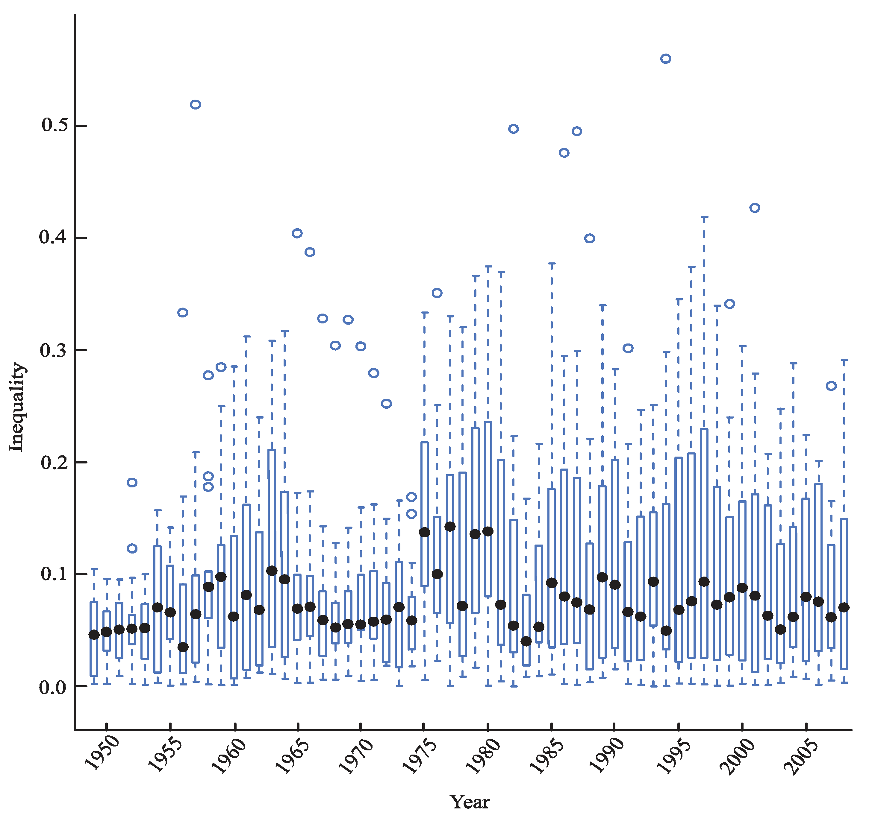
5.1. Regional Inequalities

| Year | Northeast | Lake States | Corn Belt | Northern Plains | Appalachia | Southeast | Delta | Southern Plains | Mountain | Pacific States |
|---|---|---|---|---|---|---|---|---|---|---|
| 1950 | 75.3 | 9.4 | 46.2 | 20.1 | 3.7 | 86.6 | 61.7 | 5.2 | 104.2 | 2.2 |
| 1951 | 73.1 | 31.7 | 44.8 | 48.7 | 2.0 | 57.5 | 68.9 | 16.8 | 66.7 | 3.0 |
| 1952 | 51.9 | 25.2 | 93.2 | 35.7 | 9.3 | 74.2 | 64.1 | 25.5 | 79.7 | 12.9 |
| 1953 | 63.9 | 2.0 | 57.9 | 51.4 | 39.0 | 21.5 | 23.0 | 37.7 | 181.7 | 13.7 |
| 1954 | 51.9 | 1.3 | 62.3 | 23.9 | 37.9 | 73.3 | 74.6 | 1.3 | 89.2 | 24.1 |
| 1955 | 100.0 | 12.1 | 25.0 | 26.3 | 3.0 | 151.2 | 70.3 | 4.6 | 146.2 | 6.6 |
| 1956 | 42.1 | 13.8 | 75.5 | 126.7 | 65.9 | 107.7 | 52.5 | 0.6 | 131.3 | 14.6 |
| 1957 | 24.1 | 7.8 | 65.5 | 12.0 | 28.3 | 333.4 | 1.7 | 5.1 | 90.9 | 35.0 |
| 1958 | 21.0 | 6.0 | 82.1 | 27.3 | 64.2 | 519.0 | 4.2 | 4.0 | 99.0 | 24.9 |
| 1959 | 102.6 | 4.7 | 88.7 | 99.0 | 60.9 | 277.3 | 1.7 | 1.6 | 187.2 | 81.2 |
| 1960 | 123.0 | 0.9 | 82.3 | 125.9 | 34.4 | 284.8 | 7.2 | 9.1 | 249.8 | 107.8 |
| 1961 | 129.1 | 7.0 | 26.8 | 4.5 | 25.0 | 285.3 | 2.7 | 1.3 | 146.7 | 104.5 |
| 1962 | 118.4 | 7.6 | 31.1 | 11.6 | 15.4 | 312.1 | 9.8 | 14.6 | 162.1 | 206.2 |
| 1963 | 110.6 | 24.7 | 30.3 | 13.0 | 18.7 | 239.8 | 12.5 | 12.2 | 176.7 | 132.2 |
| 1964 | 107.1 | 35.2 | 51.5 | 10.9 | 19.6 | 267.9 | 35.3 | 12.1 | 211.1 | 308.4 |
| 1965 | 97.8 | 24.2 | 37.2 | 6.7 | 25.9 | 250.5 | 33.9 | 9.9 | 173.5 | 316.9 |
| 1966 | 110.0 | 19.4 | 55.9 | 16.0 | 69.1 | 404.3 | 56.8 | 2.6 | 41.5 | 89.1 |
| 1967 | 98.3 | 13.4 | 46.2 | 32.3 | 82.9 | 387.3 | 72.9 | 3.2 | 44.9 | 71.1 |
| 1968 | 95.9 | 20.9 | 27.0 | 12.2 | 68.8 | 328.3 | 59.2 | 5.9 | 34.3 | 79.3 |
| 1969 | 103.7 | 38.4 | 16.8 | 15.5 | 62.2 | 304.1 | 63.1 | 5.8 | 41.6 | 51.4 |
| 1970 | 85.8 | 38.7 | 23.0 | 17.0 | 63.0 | 327.0 | 72.5 | 9.4 | 45.6 | 40.0 |
| 1971 | 99.6 | 51.8 | 10.0 | 17.1 | 70.5 | 303.3 | 69.8 | 4.9 | 53.0 | 50.0 |
| 1972 | 105.3 | 68.9 | 20.3 | 26.1 | 55.5 | 279.3 | 83.6 | 5.5 | 52.9 | 42.5 |
| 1973 | 106.3 | 54.1 | 18.4 | 19.8 | 81.9 | 252.1 | 69.7 | 21.5 | 59.3 | 20.6 |
| 1974 | 143.6 | 0.1 | 10.8 | 155.5 | 15.3 | 7.0 | 65.9 | 17.1 | 82.5 | 47.9 |
| 1975 | 153.7 | 17.7 | 79.7 | 49.2 | 65.8 | 32.9 | 21.3 | 62.3 | 53.2 | 26.1 |
| 1976 | 123.2 | 37.4 | 26.4 | 220.5 | 27.9 | 169.4 | 17.6 | 5.5 | 89.3 | 26.0 |
| 1977 | 102.0 | 37.8 | 51.1 | 83.4 | 97.6 | 127.9 | 35.7 | 22.7 | 160.0 | 65.5 |
| 1978 | 201.2 | 56.6 | 42.2 | 21.1 | 113.5 | 330.1 | 31.9 | 0.2 | 163.7 | 173.4 |
| 1979 | 281.5 | 26.7 | 88.1 | 16.3 | 8.6 | 190.5 | 38.6 | 63.1 | 82.2 | 14.1 |
| 1980 | 106.6 | 35.8 | 30.3 | 65.5 | 38.0 | 306.6 | 16.6 | 60.1 | 264.4 | 87.5 |
| 1981 | 86.3 | 80.2 | 64.5 | 88.0 | 14.0 | 238.7 | 60.4 | 0.5 | 216.0 | 341.5 |
| 1982 | 202.1 | 57.0 | 36.9 | 15.9 | 81.4 | 369.6 | 4.4 | 21.6 | 117.4 | 61.1 |
| 1983 | 158.9 | 54.0 | 37.5 | 16.9 | 39.9 | 497.2 | 20.9 | 0.0 | 138.2 | 30.3 |
| 1984 | 74.4 | 8.3 | 19.0 | 16.6 | 26.0 | 167.4 | 18.6 | 10.2 | 108.0 | 44.0 |
| 1985 | 111.1 | 53.0 | 51.2 | 18.4 | 39.1 | 216.3 | 26.1 | 8.9 | 125.4 | 40.1 |
| 1986 | 115.4 | 65.9 | 66.3 | 10.6 | 34.7 | 377.1 | 33.1 | 32.0 | 179.8 | 115.9 |
| 1987 | 147.1 | 67.6 | 80.0 | 7.6 | 37.7 | 476.1 | 10.4 | 1.8 | 202.0 | 73.7 |
| 1988 | 170.1 | 38.6 | 54.5 | 6.1 | 45.4 | 495.0 | 5.2 | 1.2 | 185.8 | 74.9 |
| 1989 | 127.5 | 10.3 | 27.8 | 15.5 | 102.2 | 399.8 | 3.6 | 5.9 | 119.3 | 15.2 |
| 1990 | 137.6 | 22.8 | 32.9 | 25.5 | 97.4 | 339.9 | 9.8 | 7.6 | 178.9 | 141.4 |
| 1991 | 202.0 | 27.6 | 34.1 | 36.3 | 74.6 | 225.7 | 15.2 | 16.4 | 211.0 | 142.8 |
| 1992 | 92.0 | 14.3 | 32.4 | 22.1 | 127.9 | 301.5 | 2.0 | 2.8 | 128.7 | 37.4 |
| 1993 | 229.4 | 23.3 | 44.7 | 2.9 | 113.4 | 151.5 | 8.0 | 0.9 | 107.5 | 27.7 |
| 1994 | 133.3 | 82.0 | 18.5 | 48.1 | 74.2 | 179.0 | 0.0 | 0.4 | 201.8 | 54.1 |
| 1995 | 162.8 | 26.3 | 54.0 | 2.3 | 45.8 | 45.4 | 49.4 | 0.2 | 560.1 | 32.7 |
| 1996 | 203.8 | 19.7 | 21.2 | 22.2 | 68.2 | 345.4 | 7.3 | 2.5 | 260.0 | 41.0 |
| 1997 | 207.7 | 26.4 | 25.3 | 9.8 | 67.8 | 374.3 | 2.2 | 2.6 | 317.7 | 75.8 |
| 1998 | 229.3 | 52.6 | 25.3 | 7.9 | 86.3 | 418.8 | 2.3 | 1.6 | 330.5 | 93.5 |
| 1999 | 160.4 | 51.7 | 23.5 | 6.0 | 72.7 | 284.7 | 6.1 | 0.4 | 339.7 | 32.4 |
| 2000 | 120.6 | 63.4 | 28.1 | 23.1 | 79.2 | 198.4 | 14.3 | 0.5 | 341.0 | 52.5 |
| 2001 | 158.3 | 81.6 | 20.9 | 16.1 | 100.7 | 234.4 | 22.9 | 2.2 | 303.4 | 35.8 |
| 2002 | 279.1 | 12.2 | 12.5 | 14.7 | 97.5 | 426.8 | 4.9 | 0.7 | 226.5 | 30.4 |
| 2003 | 161.3 | 30.5 | 14.7 | 24.6 | 70.8 | 207.4 | 13.6 | 0.8 | 181.0 | 24.1 |
| 2004 | 127.0 | 50.5 | 48.1 | 6.1 | 89.2 | 20.5 | 11.2 | 3.0 | 247.6 | 33.1 |
| 2005 | 94.4 | 50.6 | 34.9 | 8.3 | 202.0 | 61.9 | 59.0 | 15.9 | 288.4 | 24.2 |
| 2006 | 113.7 | 22.4 | 12.9 | 6.6 | 167.4 | 219.1 | 30.8 | 6.4 | 224.1 | 31.7 |
| 2007 | 100.3 | 40.8 | 9.2 | 19.1 | 180.3 | 188.1 | 31.2 | 1.2 | 201.0 | 39.6 |
| 2008 | 59.5 | 33.7 | 14.6 | 33.9 | 165.2 | 125.7 | 5.2 | 6.2 | 267.9 | 61.5 |
| 2009 | 129.7 | 11.3 | 14.7 | 44.4 | 150.8 | 291.3 | 15.2 | 3.2 | 220.3 | 26.4 |
| Northeast | Lake States | Corn Belt | Northern Plains | Appalachia | Southeast | Delta | Southern Plains | Mountain | Pacific States | |
|---|---|---|---|---|---|---|---|---|---|---|
| Full Sample | ||||||||||
| Min | 21.0 | 0.1 | 9.2 | 2.3 | 2.0 | 7.0 | 0.0 | 0.0 | 34.3 | 2.2 |
| Quartile 1 | 97.3 | 13.1 | 24.9 | 11.9 | 32.9 | 163.4 | 7.3 | 1.5 | 90.5 | 26.3 |
| Median | 112.4 | 26.6 | 41.1 | 18.8 | 65.0 | 260.0 | 22.1 | 5.2 | 162.9 | 41.8 |
| Quartile 3 | 154.9 | 52.0 | 76.6 | 34.4 | 83.8 | 330.9 | 59.5 | 12.1 | 217.1 | 79.8 |
| Max | 281.5 | 37.4 | 230.3 | 220.5 | 202.0 | 519.0 | 17.6 | 63.1 | 560.1 | 341.5 |
| Mean | 125.1 | 35.2 | 56.8 | 33.1 | 65.4 | 249.5 | 34.9 | 10.2 | 168.2 | 68.6 |
| Std. Dev. | 55.0 | 29.1 | 48.6 | 40.3 | 45.2 | 130.1 | 37.1 | 14.5 | 97.9 | 72.2 |
| 1950–1995 Subsample | ||||||||||
| Min | 21.0 | 0.1 | 10.0 | 2.3 | 2.0 | 7.0 | 0.0 | 0.0 | 34.3 | 2.2 |
| Quartile 1 | 93.0 | 10.8 | 32.5 | 13.6 | 25.9 | 155.5 | 9.8 | 2.0 | 82.3 | 26.0 |
| Median | 106.9 | 25.0 | 52.8 | 20.0 | 42.7 | 272.6 | 33.5 | 5.9 | 127.1 | 49.0 |
| Quartile 3 | 136.5 | 52.7 | 82.3 | 45.2 | 70.2 | 329.7 | 63.9 | 16.0 | 179.6 | 88.7 |
| Max | 281.5 | 137.4 | 230.3 | 220.5 | 127.9 | 519.0 | 217.6 | 63.1 | 560.1 | 341.5 |
| Mean | 116.5 | 34.0 | 67.4 | 37.9 | 50.6 | 251.6 | 40.6 | 12.2 | 137.9 | 76.3 |
| Std. Dev. | 51.1 | 31.4 | 50.7 | 44.6 | 32.5 | 133.2 | 39.9 | 15.9 | 87.9 | 80.3 |
| 1996–2009 Subsample | ||||||||||
| Min | 59.5 | 11.3 | 9.2 | 6.0 | 67.8 | 20.5 | 2.2 | 0.4 | 181.0 | 24.1 |
| Quartile 1 | 115.4 | 23.4 | 14.6 | 8.0 | 74.3 | 190.7 | 5.4 | 0.9 | 224.7 | 30.7 |
| Median | 144.0 | 37.3 | 21.1 | 15.4 | 93.4 | 226.8 | 12.4 | 2.4 | 264.0 | 34.5 |
| Quartile 3 | 193.2 | 51.4 | 25.3 | 22.9 | 161.6 | 331.9 | 21.0 | 3.2 | 314.1 | 49.6 |
| Max | 279.1 | 81.6 | 48.1 | 44.4 | 202.0 | 426.8 | 59.0 | 15.9 | 341.0 | 93.5 |
| Mean | 153.2 | 39.1 | 21.9 | 17.3 | 114.2 | 242.6 | 16.2 | 3.4 | 267.8 | 43.0 |
| Std. Dev. | 59.6 | 20.4 | 10.4 | 11.5 | 47.9 | 123.9 | 15.6 | 4.1 | 53.3 | 20.8 |
| Regression Results | ||||||||||
| Constant | 72.31 | −3.82 | −122.69 * 1 | −129.64 | 39.74 | 854.44 ** | −36.64 | −47.29 ** | 187.40 | 157.49 |
| (107.10) 2 | (60.95) | (167.88) | (153.80) | (62.12) | (843.20) | (95.41) | (66.28) | (247.73) | (168.79) | |
| Trend | 1.98 ** | 1.09 ** | 2.24 ** | 1.60 | 1.15 ** | −5.39 ** | 0.27 | 0.68 ** | 0.86 | −0.67 |
| (2.04) | (1.34) | (2.75) | (1.90) | (1.43) | (5.60) | (1.22) | (0.87) | (2.32) | (1.57) | |
| FAIR | −23.51 | −22.39 ** | −55.78 ** | −14.61 | 22.48 | −44.59 | −3.24 | −11.17 ** | 75.30 | −40.35 |
| (32.92) | (26.92) | (60.39) | (19.10) | (28.50) | (77.99) | (18.30) | (13.32) | (95.59) | (54.00) | |
| Prices Received | −0.01 | 0.06 | 0.71 ** | 0.67 ** | −0.08 | −2.46 ** | 0.37 | 0.23 *** | −0.36 | −0.34 |
| (0.28) | (0.24) | (0.86) | (0.75) | (0.21) | (2.43) | (0.50) | (0.30) | (0.65) | (0.42) | |
5.2. Aggregate Inequalities
| Year | Regional Inequality | Average Inequality | Total Inequality |
|---|---|---|---|
| 1950 | 68.7 | 35.9 | 104.4 |
| 1951 | 58.2 | 37.6 | 95.6 |
| 1952 | 44.9 | 50.6 | 95.1 |
| 1953 | 43.0 | 54.4 | 96.8 |
| 1954 | 57.7 | 42.0 | 100.1 |
| 1955 | 92.2 | 65.7 | 157.2 |
| 1956 | 79.6 | 62.0 | 141.8 |
| 1957 | 114.3 | 54.4 | 169.4 |
| 1958 | 134.2 | 74.0 | 208.9 |
| 1959 | 90.6 | 87.2 | 177.8 |
| 1960 | 92.7 | 97.5 | 190.1 |
| 1961 | 134.2 | 62.3 | 197.0 |
| 1962 | 118.7 | 81.5 | 200.9 |
| 1963 | 137.3 | 68.2 | 206.1 |
| 1964 | 157.2 | 103.3 | 261.3 |
| 1965 | 150.6 | 95.5 | 246.8 |
| 1966 | 99.5 | 72.0 | 172.5 |
| 1967 | 104.1 | 68.8 | 173.8 |
| 1968 | 84.7 | 57.0 | 142.7 |
| 1969 | 74.4 | 52.4 | 128.0 |
| 1970 | 84.5 | 55.7 | 141.4 |
| 1971 | 102.8 | 55.2 | 159.6 |
| 1972 | 103.0 | 57.5 | 162.2 |
| 1973 | 92.0 | 55.4 | 149.7 |
| 1974 | 95.4 | 70.6 | 165.7 |
| 1975 | 110.2 | 58.8 | 169.0 |
| 1976 | 196.7 | 136.8 | 333.4 |
| 1977 | 250.6 | 100.0 | 351.1 |
| 1978 | 188.3 | 117.0 | 306.0 |
| 1979 | 248.6 | 71.6 | 320.5 |
| 1980 | 216.9 | 149.0 | 366.1 |
| 1981 | 235.7 | 138.3 | 374.5 |
| 1982 | 204.5 | 72.8 | 278.3 |
| 1983 | 148.5 | 73.1 | 223.5 |
| 1984 | 81.7 | 40.1 | 123.0 |
| 1985 | 150.7 | 58.5 | 211.2 |
| 1986 | 176.2 | 92.3 | 270.9 |
| 1987 | 193.4 | 98.0 | 294.8 |
| 1988 | 202.7 | 92.4 | 299.2 |
| 1989 | 149.0 | 68.6 | 220.7 |
| 1990 | 178.5 | 89.7 | 271.2 |
| 1991 | 189.5 | 90.6 | 282.9 |
| 1992 | 147.3 | 66.3 | 216.4 |
| 1993 | 181.5 | 62.2 | 246.7 |
| 1994 | 155.3 | 93.3 | 251.0 |
| 1995 | 193.7 | 102.6 | 298.5 |
| 1996 | 152.5 | 86.3 | 241.1 |
| 1997 | 164.3 | 98.9 | 265.6 |
| 1998 | 172.3 | 108.6 | 283.0 |
| 1999 | 177.7 | 87.7 | 267.2 |
| 2000 | 151.1 | 87.1 | 239.9 |
| 2001 | 164.9 | 87.7 | 254.7 |
| 2002 | 80.6 | 89.2 | 171.2 |
| 2003 | 114.0 | 62.9 | 178.3 |
| 2004 | 130.7 | 66.3 | 198.5 |
| 2005 | 142.2 | 83.6 | 227.3 |
| 2006 | 122.1 | 79.7 | 202.8 |
| 2007 | 116.5 | 75.3 | 192.9 |
| 2008 | 84.0 | 78.8 | 163.5 |
| 2009 | 70.1 | 78.7 | 149.3 |
| Year | Regional Inequality | Average Inequality | Total Inequality |
|---|---|---|---|
| Constant | 96.45 1 | 46.43 * | 147.00 |
| (111.59) 2 | (69.16) | (177.80) | |
| Trend | 2.34 ** | 0.85 ** | 3.21 ** |
| (2.63) | (0.84) | (3.89) | |
| FAIR | −80.54 ** | −13.86 | −95.72 ** |
| (87.00) | (16.07) | (99.05) | |
| Prices Received | −0.08 | 0.05 | −0.05 |
| (0.27) | (0.14) | (0.46) |
6. Conclusions
Acknowledgements
References
- Theil, H. Economics and Information Theory; North-Holland Publishing Co.: Amsterdam, The Netherlands, 1967. [Google Scholar]
- Schmitz, A.; Moss, C.B.; Schmitz, T.G.; Furtan, H.W.; Schmitz, H.C. Agricultural Policy, Agribusiness, and Rent-Seeking Behaviour; University of Toronto Press: Toronto, ON, Canada, 2010. [Google Scholar]
- Moss, C.B.; Schmitz, A. Government Policy and Farmland Markets: The Maintenance of Farmer Wealth; Iowa State University Press: Ames, IA, USA, 2003. [Google Scholar]
- Reynolds, J.E.; Timmons, J.F. Factors Affecting Farmland Values in the United States; Research Bulletin No. 566; Iowa State University Agricultural Experiment Station: Ames, IA, USA, 1969. [Google Scholar]
- Duffy, P.A.; Taylor, C.R.; Casin, D.L.; Young, G.L. The Economic Value of Farm Program Base. Land Econ. 1994, 70, 318–329. [Google Scholar]
- Harris, D.G. Inflation-Indexes, Price Supports, and Land Values. Am. J. Agr. Econ. 1977, 59, 489–495. [Google Scholar]
- Herriges, D.H.; Barikman, N.E.; Shogren, J.F. The Implicit Value of Corn Base Acreage. Am. J. Agr. Econ. 1992, 74, 50–58. [Google Scholar] [CrossRef]
- Barnard, C.; Nehring, R.; Ryan, J.; Collender, R. Higher Cropland Value from Farm Program Payments: Who Gains. Agr. Outlook 2001, November, 26–30. [Google Scholar]
- Gardner, B.L. U.S. Commodity Policies and Land Prices; Technical Report WP 02-02; University of Maryland: College Park, MD, USA, 2002. [Google Scholar]
- Weersink, A.; Clark, S.; Turvey, C.G.; Sarker, R. The Effect of Agricultural Policy on Farmland Values. Land Econ. 1999, 75, 425–439. [Google Scholar] [CrossRef]
- Shaik, S.; Atwood, J.A.; Helmers, G.A. The Evolution of Farm Programs and their Contribution to Agricultural Land Values. Am. J. Agr. Econ. 2005, 87, 1190–1197. [Google Scholar] [CrossRef]
- Mason, J.E. Acreage Allotments and Land Prices. J. Land Public Utility Econ. 1968, 22, 176–181. [Google Scholar] [CrossRef]
- Seagraves, J.A. Capitalized Values of Tobacco Allotments and the Rate of Return to Allotment Holders. Am. J. Agr. Econ. 1969, 51, 320–334. [Google Scholar] [CrossRef]
- Tweeten, L.; Martin, J.E. A Methodology for Predicting U.S. Farm Real Estate Price Variations. J. Farm Econ. 1976, 42, 378–393. [Google Scholar] [CrossRef]
- Herdt, R.; Cochrane, W. Farm Land Prices and Farm Technology Advance. J. Farm Econ. 1966, 48, 243–263. [Google Scholar] [CrossRef]
- Melichar, E. Capital Gains versus Current Income in the Farming Sector. Am. J. Agr. Econ. 1979, 61, 1086–1106. [Google Scholar] [CrossRef]
- Traill, W.B. Land Values and Rents: The Gains and Losses from Farm Price Support Programmes; Department of Agricultural Economics Bulletin No. 175; University of Manchester: Manchester, UK, 1980. [Google Scholar]
- Clark, J.S.; Klein, K.K.; Thompson, S.J. Are Subsidies Capitalized into Land Values? Some Time Series Evidence from Saskatchewan. Can. J. Agr. Econ. 1993, 41, 55–163. [Google Scholar] [CrossRef]
- Just, R.E.; Miranowski, J.A. Understanding Farmland Price Changes. Am. J. Agr. Econ. 1993, 75, 156–168. [Google Scholar] [CrossRef]
- Moss, C.B.; Shonkwiler, J.S.; Reynolds, J.E. Government Payments to Farmers and Real Agricultural Asset Values in the 1980s. South. J. Agr. Econ. 1989, 21, 139–153. [Google Scholar]
- Featherstone, A.M.; Baker, T.G. Effects of Reduced Price and Income Supports on Farmland Rents and Values. NC J. Agr. Econ. 1988, 10, 177–190. [Google Scholar]
- Alston, J.M. An Analysis of Growth of U.S. Farmland Prices, 1963–1982. Am. J. Agr. Econ. 1986, 68, 1–9. [Google Scholar] [CrossRef]
- Burt, O.R. Econometric Modeling of the Capitalization Formula for Farmland Prices. Am. J. Agr. Econ. 1986, 68, 10–26. [Google Scholar] [CrossRef]
- Pope, R.D.; Kramer, R.A.; Green, R.D.; Gardner, B.D. An Evaluation of Economic Models of U.S. Farmland Prices. West. J. Agr. Econ. 1978, 4, 107–119. [Google Scholar]
- Palmquist, R.B.; Danielson, L.E. A Hedonic Study of the Effects of Erosion Control and Drainage on Farmland Values. Am. J. Agr. Econ. 1989, 71, 55–62. [Google Scholar] [CrossRef]
- Shonkwiler, J.S.; Reynolds, J.E. A Note of the Use of Hedonic Price Models in the Analysis of Land Prices at the Urban Fringe. Am. J. Agr. Econ. 1986, 69, 58–63. [Google Scholar] [CrossRef]
- Xu, F.; Mittelhammer, R.C.; Barkley, P.W. Measuring the Contributions of Site Characteristics to the Value of Agricultural Land. Land Econ. 1993, 69, 356–369. [Google Scholar] [CrossRef]
- Goodwin, B.K.; Ortalo-Magne, F.N. The Capitalization of Wheat Subsidies into Agricultural Land Values. Can. J. Agr. Econ. 1992, 40, 37–54. [Google Scholar] [CrossRef]
- Goodwin, B.K.; Mishra, A.K.; Ortalo-Magne, F.N. What’s Wrong with Our Models of Agricultural Land Values. Am. J. Agr. Econ. 2003, 85, 744–752. [Google Scholar] [CrossRef]
- Vantreese, V.L.; Reed, M.R.; Skees, J.R. Production Controls and Asset Values. Am. J. Agr. Econ. 1989, 71, 319–325. [Google Scholar] [CrossRef]
- Moss, C.B. Returns, Interest Rates, and Inflation: How They Explain Changes in Farmland Values. Am. J. Agr. Econ. 1997, 79, 1311–1318. [Google Scholar] [CrossRef]
- Lindon, J.R.; Lins, D.A.; Venkataraman, R. Cash Rents and Land Values in U.S. Agriculture. Am. J. Agr. Econ. 1985, 67, 794–805. [Google Scholar]
- Shaik, S. Farm Programs and Land Values in Mountain States: Alternative Panel Estimators. In Proceedings of the WAEA Annual Meetings, Portland, OR, USA, 29 July 2007.
- Falk, B. Formally Testing the Present Value Model of Farmland Prices. Am. J. Agr. Econ. 1991, 73, 1–10. [Google Scholar] [CrossRef]
- Lence, S.H.; Mishra, A.K. The Impacts of Different Farm Programs on Cash Rents. Am. J. Agr. Econ. 2003, 85, 753–761. [Google Scholar] [CrossRef]
- Shaik, S.; Miljkovic, D. Dynamic Relationships Between Farm Real Estate Values and Federal Farm Program Payments. J. Agr. Resour. Econ. 2010, 35, 153–165. [Google Scholar]
- Goodwin, B.K.; Mishra, A.K.; Ortalo-Magne, F.N. The Buck Stops Where? The Distribution of Agricultural Subsidies; NBER Working Paper 16693; National Bureau of Economic Research: Cambridge, MA, USA, 2011.
- USDA/NASS. Land Values and Cash Rents. United States Deparment of Agriculture: Washington, DC, USA, 2010. [Google Scholar]
- USDA/NASS. Data and Statistics: Quickstats. United States Department of Agriculture: Washington, DC, USA, 2010. [Google Scholar]
- Theil, H.; Chung, C.-F.; Seale, J.L., Jr. International Evidence on Consumption Patterns; JAI Press: Greenwich, CT, USA, 1989. [Google Scholar]
- Efron, B. Bootstrap Methods: Another Look at the Jackknife. Ann. Statist. 1979, 7, 1–26. [Google Scholar] [CrossRef]
- Efron, B. Nonparametric Estimates of Standard Error: The Jackknife, the Bootstrap, and Other Methods. Biometrika 1981, 68, 589–599. [Google Scholar] [CrossRef]
© 2011 by the authors; licensee MDPI, Basel, Switzerland. This article is an open access article distributed under the terms and conditions of the Creative Commons Attribution license (http://creativecommons.org/licenses/by/3.0/).
Share and Cite
Mishra, A.K.; Livanis, G.T.; Moss, C.B. Did the Federal Agriculture Improvement and Reform Act of 1996 Affect Farmland Values? Entropy 2011, 13, 668-682. https://doi.org/10.3390/e13030668
Mishra AK, Livanis GT, Moss CB. Did the Federal Agriculture Improvement and Reform Act of 1996 Affect Farmland Values? Entropy. 2011; 13(3):668-682. https://doi.org/10.3390/e13030668
Chicago/Turabian StyleMishra, Ashok K., Grigorios T. Livanis, and Charles B. Moss. 2011. "Did the Federal Agriculture Improvement and Reform Act of 1996 Affect Farmland Values?" Entropy 13, no. 3: 668-682. https://doi.org/10.3390/e13030668
APA StyleMishra, A. K., Livanis, G. T., & Moss, C. B. (2011). Did the Federal Agriculture Improvement and Reform Act of 1996 Affect Farmland Values? Entropy, 13(3), 668-682. https://doi.org/10.3390/e13030668