Article

Estimation of Seismic Wavelets Based on the Multivariate Scale Mixture of Gaussians Model

Institute of Waves and Information, School of Electronics and Information Engineering, Xi’an Jiaotong University, No.28 of West Xian’ning Road, Xi’an 710049, China
*
Author to whom correspondence should be addressed.
Entropy 2010, 12(1), 14-33; https://doi.org/10.3390/e12010014
Submission received: 9 October 2009 / Accepted: 11 December 2009 / Published: 28 December 2009
(This article belongs to the Special Issue Maximum Entropy)

Abstract

:
This paper proposes a new method for estimating seismic wavelets. Suppose a seismic wavelet can be modeled by a formula with three free parameters (scale, frequency and phase). We can transform the estimation of the wavelet into determining these three parameters. The phase of the wavelet is estimated by constant-phase rotation to the seismic signal, while the other two parameters are obtained by the Higher-order Statistics (HOS) (fourth-order cumulant) matching method. In order to derive the estimator of the Higher-order Statistics (HOS), the multivariate scale mixture of Gaussians (MSMG) model is applied to formulating the multivariate joint probability density function (PDF) of the seismic signal. By this way, we can represent HOS as a polynomial function of second-order statistics to improve the anti-noise performance and accuracy. In addition, the proposed method can work well for short time series.

1. Introduction

In seismic exploration, a seismic trace y(n) can be often represented as the convolution of a wavelet w(n) with the reflectivity series r(n) plus a superposed noise n(n):
y ( n ) = s ( n ) + n ( n ) = r ( n ) w ( n ) + n ( n )
where * denotes the convolution, s(n) represents the clean signal. It is generally assumed that reflectivity is a white super-Gaussian process; the noise is a white Gaussian process, and the wavelet is a band-limited filter.
In equation (1), the reflectivity series, the wavelet, and noise are unknown, except for the seismic trace, which can be obtained by a seismic receiver, so estimation of the wavelet and the reflectivity series from the seismic trace is a typical blind deconvolution problem.
Many techniques have previously been developed for this purpose, and these have been reviewed and described in detail in the literature. One early technique, which assumes that the reflectivity sequence is a Gaussian white noise, supplies a minimum phase wavelet from the second-order statistical content of the trace signal [1,2]. Unfortunately, this approach is not satisfactory since the source wavelet is usually non-minimum phase, and the reflectivity sequence is not well described by a Gaussian model.
Another way of applying the whiteness hypothesis to estimating the wavelet consists in general purpose information criteria [3,4,5,6]. It is related to minimizing the mutual information rate, which measures the independence degree of the deconvolved data sequence. Though there are some shortcomings to be overcome in the method, such as sensitivity to noise, finding global optimum, and so on, it is still a very important approach due to the absence of limitations for the wavelet phase.
In the blind deconvolution context, the problem is ill posed, and extra assumptions about the reflectivity or about the wavelet are necessary. For instance, one can model the reflectivity sequence by using a Bernoulli-Gaussian (BG) model. In the literature, a few approaches based on spike detection/estimation and BG models have been proposed using a maximum-likelihood approach or in a Bayesian framework adding some priors [7,8,9]. For seismic field data, the reflectivity sequence changes do not appear as clearly as predicted by the BG model, therefore, the sparse nature of the input signal is not a sufficiently robust hypothesis for good system estimation [3].
The cumulant matching (CM) method has been developed for estimating a mix-phase wavelet from a convolutional process [10]. Matching between the trace cumulant and the wavelet moment is done in a minimum mean-squared error sense under the assumption of a non-Gaussian, stationary and statistically independent reflectivity sequence. The reliability of the Higher-order Statistics (HOS) matching method depends strongly on the amount of data available. Thus, in this paper, we are interested in the problem of how we can estimate the HOS from the field recordings accurately and efficiently without having a large amount of data available. A computationally efficient method is proposed for computing the HOS (fourth-order and sixth-order cumulants) based on the joint probability distribution function (PDF) of the output seismic signal, which is described by the multivariate scale mixture of Gaussians (MSMG) model. Using this PDF model, we can represent HOS as a polynomial function of Second-order Statistics (SOS); hence we work just with SOS. Since SOS is phaseless, we apply constant-phase rotations technique to estimating the wavelet phase. Simulation result is provided showing the performance of the method, and the proposed method is seen to work satisfactorily in a real data example.
This paper is organized as follows. In Section 2, we describe the wavelet model and introduce the general CM methods for estimating the wavelet parameters. After introducing MSMG PDF model briefly in Section 3, and in Section 4, we derive the cumulants of the field recordings from second-order to sixth-order based on MSMG model, and use the one-dimensional cumulant rate (ODCR) to match the one-dimensional rate of the wavelet moment in order to obtain the scale and frequency parameters of the wavelet; we then illustrate performances of different orders ODCR for estimating the wavelet. In Section 5, we describe our wavelet estimation procedure. Examples illustrating the effectiveness of our approach are given in Section 6. Finally, we summarize our work in Section 7.

2. Wavelet Model and the General CM Methods

In reservoir geophysics, the seismic wavelet usually can be approximated by a formula as follows [11]:
w ( t ) = e ( t σ ) 2 cos ( 2 π f t + φ )
where the scale, σ, controls the width of the seismic wavelet, φ is its initial phase and f is its dominant frequency. Without loss of generality, we let the amplitude of the wavelet be a unit.

2.1. Estimating the Phase

The optimum phase could be estimated by applying a series of constant-phase rotations to the analyzed seismic trace [12]. The rotated trace yrot(n) can be obtained from the original trace y(n) by
y r o t ( n ) = cos φ y ( n ) + sin φ H [ y ( n ) ]
where φ denotes the phase rotation angle, and H[∙] is the Hilbert transform. Since a zero-phase wavelet contains the majority of its energy in relatively narrow time duration, its kurtosis is larger than that of any non-zero-phase wavelet. So, when the kurtosis of yrot(n) reaches its maximum, the related angle, φ is considered as the most likely negative wavelet phase of y(n). This method for estimating the phase of a seismic wavelet is called the constant-phase rotation method, which is very important to the blind deconvolution of seismic traces.
The constant-phase rotation method is based on the theory of entropy. The operation of rotating the seismic trace results in the increase of its non-Gaussianity. Negentropy is used to measure the non-Gaussianity of a random variable, which is defined as:
H n e g ( X ) = H ( X G a u s s ) H ( X )
where H(X) denotes the entropy of random variable X, XGauss is a Gaussian variable with the same variance as that of X. Negentropy is nonnegative, and will become larger as a random variable goes off the Gaussianity.
In practice, the negentropy of a random variable with zero mean and unit variance can approximately be obtained as follows [13]:
H n e g ( X ) 1 12 E ( X 3 ) 2 + 1 48 k u r t 2 ( X )
where:
k u r t ( X ) = E ( X 4 ) 3
is defined as kurtosis of X. If X has a symmetrical probability distribution function, the equation above reduces to:
H n e g ( X ) 1 48 k u r t 2 ( X )
Hence, the constant-phase rotation method is identical to the minimum entropy deconvolution proposed by R.A. Wiggins. To guarantee scale-invariance, Wiggins adopted the standardized 4th cumulant as a criterion to performing optimization, for a random variable with zero mean, which is:
k ( X ) = E ( X 4 ) E 2 ( X 2 ) 3
The kurtosis is usually calculated by (7) for the constant-phase rotation method.

2.2. Estimating the Scale and Frequency of the Seismic Wavelet

To estimate the scale and frequency parameters, one can use various cumulants to match the wavelet moments based on the above models (1) and (2).
In model (1), based on the assumption that reflectivity is a zero-mean, non-Gaussian, stationary and statistically independent sequence, and the wavelet represents a linear, time-invariant, causal and stable filter, the resulting seismic trace is thus a zero-mean discrete stationary random process, we further assume that {y(n)} is kth-order stationary, then, we have the following formula:
c y ( k ) ( τ 1 , τ 2 , , τ k 1 ) = γ r ( k ) n w ( n ) w ( n + τ 1 ) w ( n + τ k 1 ) ( k 3 )
where:
c y ( k ) ( τ 1 , τ 2 , , τ k 1 ) = c u m ( k ) ( y ( n ) , y ( n + τ 1 ) , y ( n + τ 2 ) , , y ( n + τ k 1 ) )
denotes the joint kth-order cumulant of the random variables y(n), y(n + τ1), …, y(n + τk-1), and γr(k) denotes the kth-order cumulant of reflectivity sequence. The above equation establishes the relation between the kth-order cumulant of {y(n)} and the wavelet, which was proposed in 1955 by Bartlett [14] and in 1967 by Brillinger and Rosenblatt [15].
Since the reflectivity sequence distribution is unknown, γr(k) cannot be obtained, we have to match the wavelet by means of the ratio of cy(k)(τ1, τ2, …, τk-1) to cyk, where:
c y k = c y ( k ) ( τ 1 , τ 2 , , τ k 1 ) | τ 1 = τ 2 = = τ k 1 = 0
Hence, following from (8), we have:
r y ( k ) ( τ 1 , τ 2 , , τ k 1 ) = c y ( k ) ( τ 1 , τ 2 , , τ k 1 ) c y k = n w ( n ) w ( n + τ 1 ) w ( n + τ k 1 ) n w k ( n )
So, the cumulant matching method can be performed in a minimum mean-squared error sense by defining the cost function:
J = τ 1 , τ 2 , , τ k 1 | r ^ y ( k ) ( τ 1 , τ 2 , , τ k 1 ) n w ( n ) w ( n + τ 1 ) w ( n + τ k 1 ) n w k ( n ) |
where r ^ y(k)(τ1, τ2, …, τk-1) denotes the estimate of ry(k)(τ1, τ2, …, τk-1).

3. MSMG (Multivariate Scale Mixture of Gaussians) Model

In many real world data sets involving multivariate observations, the data have an empirical distribution which is highly peaked at zero (or the mean vector), and which asymptotically falls off more slowly than the Gaussian distribution as the distance from zero increases. We deal these distributions with sparse distributions, which can be frequently encountered in various areas, like blind source separation and independent component analysis (ICA), etc. Multivariate observations, which are mutually correlated and have higher-order dependencies, have frequently been represented using mixture of Gaussians models. In the above blind deconvolution context, the reflectivity sequence is said a white sparse distribution. As a convolution of a wavelet with the reflectivity series, the clean signal presents sparse and correlated nature, and can also be represented using mixture of Gaussians models. A random vector Y with zero mean called Multivariate scale mixture of Gaussians distribution can be described as follows [16,17,18].
Let X be an N-dimensional, zero mean Gaussian variable with covariance matrix equal to the identity matrix. And furthermore let ΓRN×N (N × N real matrix) be a positive definite symmetric matrix with det(Γ) = 1, and let Z be a scalar random variable with PDF gz(z), which can attain only positive values. We denote variable Y a multivariate scale mixture of Gaussians according to:
Y = Z Γ 1 / 2 X
Given a PDF gz(z) for the scale parameter Z, the marginal PDF for Y can be obtained by averaging the PDF of Y|Z over the density of Z:
f Y ( y ) = 0 f Y | Z ( y | z ) g Z ( z ) d z = 0 1 ( 2 π ) N / 2 z exp ( 1 2 z y T Γ 1 y ) g Z ( z ) d z
The characteristic function of Y can be written as:
Φ Y ( ω ) = E [ exp ( j y , ω ) ] = R N [ 0 1 ( 2 π ) N / 2 z exp ( 1 2 y T Γ 1 y ) g Z ( z ) d z ] exp ( j y , ω ) d y = 0 g Z ( z ) exp ( 1 2 z ω T Γ ω ) d z
where:
y = [ y 1 , y 2 , , y N ] T , ω = [ ω 1 , ω 2 , , ω N ] T .
Using (13), we have:
Φ Y ( ω ) ω = ω 0 g Z ( z ) exp ( 1 2 z ω T Γ ω ) d z = [ 0 z g Z ( z ) exp ( 1 2 z ω T Γ ω ) d z ] Γ ω
2 Φ Y ( ω ) ω ω T = [ 0 z g Z ( z ) exp ( 1 2 z ω T Γ ω ) d z ] Γ + [ 0 z 2 g Z ( z ) exp ( 1 2 z ω T Γ ω ) d z ] Γ ω ω T Γ
Hence, we have:
μ Y = Φ Y ( ω ) ω | ω = 0 = 0 , R Y = Φ Y ( ω ) ω ω T | ω = 0 = E ( z ) Γ
where μY is mean vector of Y, RY is covariance matrix of Y.

4. Estimating the HOS of Recorded Seismic Trace Based on MSMG Model

4.1. Calculating the HOS of Recorded Seismic Trace

Assuming that the clean signal s(n) is independent of additive noise n(n), using (1), we can write the characteristic function of the seismic trace as:
Φ y ( ω ) = Φ s ( ω ) Φ n ( ω )
where y = [y1, y2, …, yN]T is the N-dimensional vector formed by the seismic trace, Φs(ω) is the characteristic function of clean signal which can be given by (13), and Φn(ω) is the characteristic function of additive noise.
Noting that the noise is a white Gaussian process, we have:
Φ y ( ω ) = Φ s ( ω ) Φ n ( ω ) = Φ s ( ω ) exp ( 1 2 σ n 2 k = 1 N ω k 2 )
where σn2 is noise variance.
The cumulant-generating function of the seismic trace is:
Ψ y ( ω ) = ln Φ y ( ω ) = ln [ Φ s ( ω ) Φ n ( ω ) ] = ln [ 0 g Z ( z ) exp ( 1 2 z ω T Γ ω ) d z ] 1 2 σ n 2 k = 1 N ω k 2
It is well known that there is a relationship between the cumulant-generating function and the cumulant given by [19]:
c u m ( y 1 ν 1 , y 2 ν 2 , y N ν N ) = ( j ) r Ψ y r ( ω ) ω 1 ν 1 ω 2 ν 2 ω N ν N | ω 1 = ω 2 = = ω N = 0 , k = 1 N ν k = r
where j2 = −1.
Representation (19) plays a fundamental role in calculating the cumulant, using (18) and (19), we can calculate the cumulant of the seismic trace. The calculated cumulants of the recorded seismic trace from second-order to sixth-order are shown in Table 1, and the details are given in Appendix A.
Table 1. Calculated cumulants.
c u m ( 2 ) ( y i , y j ) Γ i j E ( Z ) + σ n 2 δ i j
c u m ( 3 ) ( y i , y j , y s ) 0
c u m ( 4 ) ( y i , y j , y s , y t ) ( Γ i j Γ s t + Γ i s Γ j t + Γ j s Γ i t ) var ( Z )
c u m ( 5 ) ( y i , y j , y s , y t , y m ) 0
c u m ( 6 ) ( y i , y j , y s , y t , y m , y n ) ( Γ i j Γ s t Γ m n + Γ i s Γ j t Γ m n + Γ j s Γ i t Γ m n + Γ i j Γ s m Γ t n + Γ i j Γ t m Γ s n + Γ i s Γ j m Γ t n + Γ i s Γ t m Γ j n + Γ j s Γ i m Γ t k + Γ j s Γ t m Γ i n + Γ i t Γ j m Γ s n + Γ s t Γ j m Γ i n + Γ s t Γ i m Γ j n + Γ j t Γ s m Γ i n + Γ j t Γ i m Γ s n + Γ i t Γ s m Γ j n ) [ E ( Z 3 ) 3 E ( Z ) E ( Z 2 ) + 2 E 3 ( Z ) ]
where Γij denotes the ith row and the jth column element of Γ.
Similarly, based on above result and using (9), we obtain the ratios of cy(k)(τ1, τ2, …, τk-1) to cyk for fourth-order and sixth-order, which are in Table 2, where ρs(ji) = Rs(ji)/Rs(0), is the correlation coefficient of s(n). The details are given in Appendix B.
Table 2. Cumulant rate.
r y ( 4 ) ( y i , y j , y s , y t ) [ ρ s ( j i ) ρ s ( t s ) + ρ s ( s i ) ρ s ( t j ) + ρ s ( j s ) ρ s ( t i ) ] / 3
r y ( 6 ) ( y i , y j , y s , y t , y m , y n ) [ ρ s ( j i ) ρ s ( t s ) ρ s ( n m ) + ρ s ( s i ) ρ s ( t j ) ρ s ( m n ) + ρ s ( j s ) ρ s ( t i ) ρ s ( m n ) + ρ s ( j i ) ρ s ( m s ) ρ s ( n t ) + ρ s ( j i ) ρ s ( t m ) ρ s ( n s ) + ρ s ( s i ) ρ s ( m j ) ρ s ( n t ) + ρ s ( s i ) ρ s ( t m ) ρ s ( n j ) + ρ s ( s j ) ρ s ( m i ) ρ s ( n t ) + ρ s ( j s ) ρ s ( m t ) ρ s ( n i ) + ρ s ( t i ) ρ s ( m j ) ρ s ( n s ) + ρ s ( s t ) ρ s ( m j ) ρ s ( n i ) + ρ s ( t s ) ρ s ( m i ) ρ s ( n j ) + ρ s ( t j ) ρ s ( m s ) ρ s ( n i ) + ρ s ( t j ) ρ s ( m i ) ρ s ( n s ) + ρ s ( t i ) ρ s ( m s ) ρ s ( n j ) ] / 15

4.2. One-dimensional Cumulant Rate

In practice, using one-dimensional cumulant rate (ODCR) is sufficient for us to estimate the wavelet parameters. To express succinctly, we denote different orders ODRC in convenient form, for instance:
r y ( K + L ) ( y n ( K ) , y n + m ( L ) ) = r y ( K + L ) ( y n , y n , , y n K , y n + m , y n + m , y n + m L )
The different orders ODRC and their relation to the corresponding one-dimensional rate of the wavelet moments, following from (10), are shown in Table 3, where m denotes time lag.
Table 3. ODCR and the rate of wavelet moment.
r y ( 4 ) ( y n ( 3 ) , y n + m ( 1 ) ) = r y ( 4 ) ( y n , y n , y n , y n + m ) = n w n 3 w n + m n w n 4 r y ( 4 ) ( y n ( 2 ) , y n + m ( 2 ) ) = r y ( 4 ) ( y n , y n , y n + m , y n + m ) = n w n 2 w n + m 2 n w n 4 r y ( 6 ) ( y n ( 5 ) , y n + m ( 1 ) ) = r y ( 6 ) ( y n , y n , y n , y n , y n , y n + m ) = n w n 5 w n + m n w n 6 r y ( 6 ) ( y n ( 4 ) , y n + m ( 2 ) ) = r y ( 6 ) ( y n , y n , y n , y n , y n + m , y n + m ) = n w n 4 w n + m 2 n w n 6 r y ( 6 ) ( y n ( 3 ) , y n + m ( 3 ) ) = r y ( 6 ) ( y n , y n , y n , y n + m , y n + m , y n + m ) = n w n 3 w n + m 3 n w n 6

4.3. Estimating ODCR

Noting that ρs(0) is equal to one, and following from Table 2, we can obtain the ODCR, which take the form:
r y ( 4 ) ( y n ( 3 ) , y n + m ( 1 ) ) = ρ s ( m )
r y ( 4 ) ( y n ( 2 ) , y n + m ( 2 ) ) = 1 3 + 2 3 ρ s 2 ( m )
r y ( 6 ) ( y n ( 5 ) , y n + m ( 1 ) ) = ρ s ( m )
r y ( 6 ) ( y n ( 4 ) , y n + m ( 2 ) ) = 1 5 + 4 5 ρ s 2 ( m )
r y ( 6 ) ( y n ( 3 ) , y n + m ( 3 ) ) = 3 5 ρ s ( m ) + 2 5 ρ s 3 ( m )
To obtain ODCR, we need to estimate ρs(m). It follows from (1) that:
R y ( m ) = σ r 2 R s ( m ) + σ n 2 δ ( m )
R y ( 0 ) = σ r 2 R s ( 0 ) + σ n 2
ρ y ( m ) = R y ( m ) R y ( 0 ) = σ r 2 R s ( m ) σ r 2 R s ( 0 ) + σ n 2 = ρ s ( m ) 1 + σ n 2 / σ r 2 R s ( 0 ) ( m 0 )
where σr2 denotes reflectivity variance, and δ(m) is Dirac function, Ry(m) and ρy(m) denote the autocorrelation function and the correlation coefficient of the seismic trace respectively. Hence, we have:
ρ s ( m ) = { ρ y ( m ) ρ y ( m ) [ 1 + ( σ r 2 R s ( 0 ) σ n 2 ) 1 ] ( m = 0 ) ( m 0 )
The term σr2Rs(0)/σn2 denotes Signal-to-Noise Ratio (SNR). In practice, usually we do not possess the clean data; we have to estimate ρy(m) as a substitution for ρs(m). It follows from (22) that the estimation error increases as the SNR drops.
Using above results, we can establish now the estimators of ODCR, which are given by:
r ^ y ( 4 ) ( y n ( 3 ) , y n + m ( 1 ) ) = ρ ^ y ( m )
r ^ y ( 4 ) ( y n ( 2 ) , y n + m ( 2 ) ) = 1 3 + 2 3 ρ ^ y 2 ( m )
r ^ y ( 6 ) ( y n ( 5 ) , y n + m ( 1 ) ) = ρ ^ y ( m )
r ^ y ( 6 ) ( y n ( 4 ) , y n + m ( 2 ) ) = 1 5 + 4 5 ρ ^ y 2 ( m )
r ^ y ( 6 ) ( y n ( 3 ) , y n + m ( 3 ) ) = 3 5 ρ ^ y ( m ) + 2 5 ρ ^ y 3 ( m )
where ρ ^ y(m) is the estimation of ρy(m).

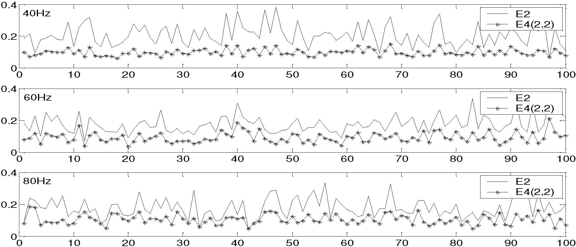
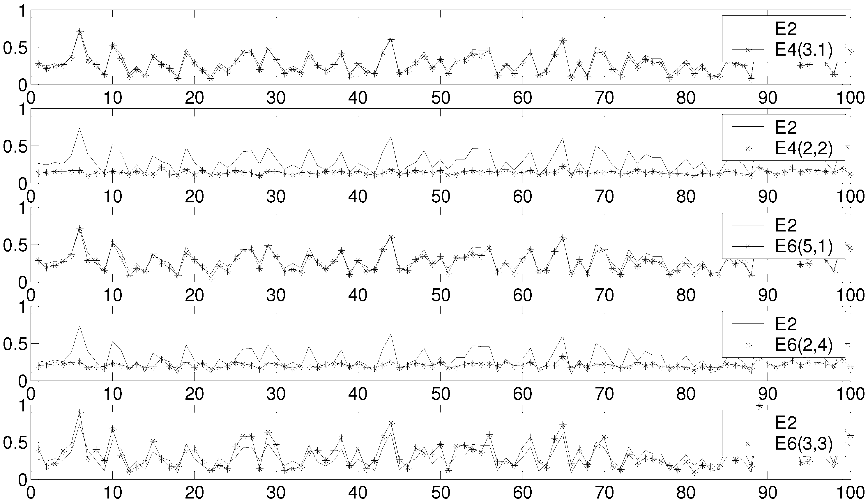
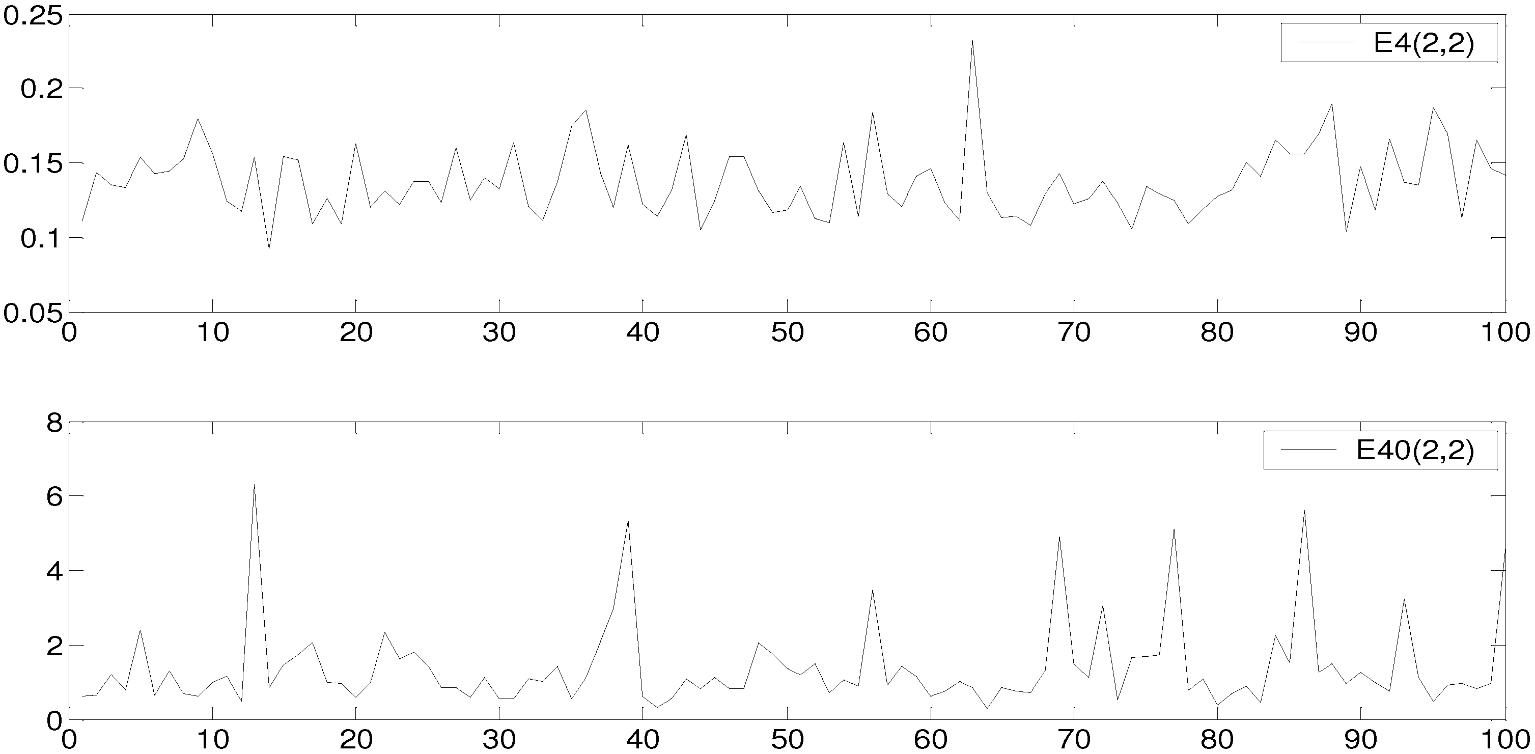
4.4. The Behavior of ODCR with Different Orders

To obtain a good estimation, it is necessary for us to exploit the differences between the different order ODCRa for matching waveleta. In this section, we thus define the different error to evaluate each estimated ODCR.
It follows from (9) and Table 3, that the value of that the true ODCR, derived from seismic data, divided by the corresponding one-dimensional rate of the wavelet moment, is equal to one. As for the estimated ODCR, the above value cannot be one, thus, we use the absolute value of the deviation from one to define error, which is shown in Table 4, where M denotes the maximal time lag.
We have simulated the seismic trace by convolving a super-Gaussian reflectivity with a seismic wavelet with zero phase, plus additive white noise, to select which one can match the wavelet best. Figure 1 illustrates the error behavior of ODCR with different orders, in terms of the summation of error, versus the number of simulation times, where the error following from correlation coefficient (the first row of Table 4) is compared with other errors from ODCR. We obtain the numerical results presented below by performing independent simulation trial 100 times. The simulation setting is shown in Table 5.
The reflectivity sequence samples are distributed according to a generalized Gaussian distribution (GGD). The PDF of a zero-mean generalized Gaussian random variable R with deviation λ is:
f R ( r ) = [ ν A ( ν , λ ) 2 Γ ˜ ( 1 / ν ) ] exp ( [ A ( ν , λ ) | r | ν ] )
where:
A ( ν , λ ) = λ 1 [ Γ ˜ ( 3 / ν ) Γ ˜ ( 1 / ν ) ] 1 / 2
where λ > 0 and Γ ˜ (∙) defines the complete Gamma function given by:
Γ ˜ ( z ) = 0 x z 1 e x d x
A(ν, λ) is a generalized measure of the variance and defines the dispersion of the distribution, while the parameter ν describes the exponential rate decay and, in general, the shape of the peak at the center of the distribution. Well-known special cases of the GGD function include a Laplacian distribution (ν = 1) and a normal distribution (ν = 2). In effect, smaller values of the shape λ correspond to heavier tails and therefore to more peaked distributions. We perform 512 Monte-Carlo runs to obtain the reflectivity sequence samples; a typical reflectivity sequence is presented in Figure 4.
Table 4. Error.
Table 4. Error.
ErrorThe summation of error
e 2 ( m ) = | 1 [ ρ ^ y ( m ) n w n 2 / n w n w n + m ] | E 2 = 1 M m = 0 M 1 e 2 ( m )
e 4 ( 3 , 1 ) ( m ) = | 1 [ r ^ y ( 4 ) ( y n ( 3 ) , y n + m ( 1 ) ) n w n 4 / n w n 3 w n + m ] | E 4 ( 3 , 1 ) = 1 M m = 0 M 1 e 4 ( 3 , 1 ) ( m )
e 4 ( 2 , 2 ) ( m ) = | 1 [ r ^ y ( 4 ) ( y n ( 2 ) , y n + m ( 2 ) ) n w n 4 / n w n 2 w n + m 2 ] | E 4 ( 2 , 2 ) = 1 M m = 0 M 1 e 4 ( 2 , 2 ) ( m )
e 6 ( 5 , 1 ) ( m ) = | 1 [ r ^ y ( 6 ) ( y n ( 5 ) , y n + m ( 1 ) ) n w n 6 / n w n 5 w n + m ] | E 6 ( 5 , 1 ) = 1 M m = 0 M 1 e 6 ( 5 , 1 ) ( m )
e 6 ( 4 , 2 ) ( m ) = | 1 [ r ^ y ( 6 ) ( y n ( 4 ) , y n + m ( 2 ) ) n w n 6 / n w n 4 w n + m 2 ] | E 6 ( 4 , 2 ) = 1 M m = 0 M 1 e 6 ( 4 , 2 ) ( m )
e 6 ( 3 , 3 ) ( m ) = | 1 [ r ^ y ( 6 ) ( y n ( 3 ) , y n + m ( 3 ) ) n w n 6 / n w n 3 w n + m 3 ] | E 6 ( 3 , 3 ) = 1 M m = 0 M 1 e 6 ( 3 , 3 ) ( m )
Table 5. Simulation setting.
σ f M ν λ SNR
0.02 s 30.3 H z 15 0.9 0.28 7.2 d B
As can be seen from Figure 1, r ^ y(4)(yn(2), yn+m(2)) gains the best performance to match the wavelet, the next is r ^ y(6)(yn(4), yn+m(2)). Moreover, in our simulation trials, the error variances of using r ^ y(4)(yn(2), yn+m(2)) and r ^ y(6)(yn(4), yn+m(2)) are very small, about 3 × 10⁻⁴ and 5 × 10⁻⁴ respectively, others are about 0.01, which implies the numerical robustness.
Figure 1. The error behavior of ODCR with different orders.
Entropy 12 00014 g001
Figure 2 shows the change of the performance of r ^ y(4)(yn(2), yn+m(2)) with the wavelet frequency. We can see that there is no distinct change when the frequency varies. Like the other methods, the smaller the value of the scale of the wavelet is, the better estimation values our method can obtain. In order to test our method, we choose a comparatively large scale value for the wavelet in the simulation.
Figure 2. The change of the performance in variation with wavelet frequency.
Entropy 12 00014 g002
To complete our discussion, we finally compare the performance of r ^ y(4)(yn(2), yn+m(2)) derived from MSMG model with that of the same one estimated directly from the recorded seismic trace. r ^ y(4)(yn(2), yn+m(2)), estimated directly from the recorded seismic trace, is denoted as r ^ y0(4)(yn(2), yn+m(2)).
According to:
r y ( 4 ) ( y n , y n , y n + m , y n + m ) = E ( y n 2 y n + m 2 ) R y 2 ( 0 ) 2 R y 2 ( m ) E ( y n 4 ) 3 R y 2 ( 0 )
we have the estimator for r ^ y0(4)(yn(2), yn+m(2)) given by:
r ^ y 0 ( 4 ) ( y n ( 2 ) , y n + m ( 2 ) ) = 1 N n = 0 N m 1 y n 2 y n + m 2 ( 1 N n = 0 N 1 y n 2 ) 2 2 ( 1 N n = 0 N m 1 y n y n + m ) 2 1 N n = 0 N 1 y n 4 3 ( 1 N n = 0 N 1 y n 2 ) 2
Similarly, we define the error and its summation in term of r ^ y0(4)(yn(2), yn+m(2)), given by:
e 40 ( 2 , 2 ) ( m ) = | r ^ y 0 ( 4 ) ( y n ( 2 ) , y n + m ( 2 ) ) n w n 4 n w n 2 w n + m 2 1 |
and:
E 40 ( 2 , 2 ) = 1 M m = 0 M 1 e 40 ( 2 , 2 ) ( m )
We also perform independent simulation trial 100 times in the same setting which is shown in Table 5, the result illustrated in Figure 3 shows that using r ^ y0(4)(yn(2), yn+m(2)) to match the wavelet is very poor, the drastically different performance with that of using r ^ y(4)(yn(2), yn+m(2)) consist in that the outliers of seismic trace pose a serious influence on the HOS estimation.
Figure 3. The error performance of r ^ y(4)(yn(2), yn+m(2)) and r ^ y0(4)(yn(2), yn+m(2)).
Entropy 12 00014 g003

5. Estimating the Wavelet

We can solve our problem in a two-step approach. First, we estimate the wavelet phase using the constant-phase rotation method. Then, we use r ^ y(4)(yn(2), yn+m(2)) to match the rate of the wavelet moment in order to obtain the scale and frequency parameters. Since the estimator of ODCR is a polynomial function of the correlation coefficient, and the correlation coefficient is phaseless, we can perform these two steps.
As for computing the rate of the wavelet moment, since correlation coefficient is phaseless, we use the wavelet by simply taking the form:
w ( t ) = e ( t σ ) 2 cos ( 2 π f t )
Its discrete moment rate corresponding to r ^ y(4)(yn(2), yn+m(2)) is:
M w , 4 ( 2 , 2 ) ( m ) = n w n 2 w n + m 2 n w n 4
Minimizing cost function:
J = m = 0 M 1 | r ^ y ( 4 ) ( y n ( 2 ) , y n + m ( 2 ) ) M w , 4 ( 2 , 2 ) ( m ) |
we can obtain the scale and frequency parameters:
[ σ ^ , f ^ ] = arg min σ , f J
This is done by simply searching for different values of the scale and frequency among their reasonable scopes, which can be obtained from the spectrum of the seismic trace. Based on above results, we summarize the seismic wavelet estimate algorithm as follows:
  • Use constant-phase rotation method to obtain the wavelet phase.
  • Estimate the correlation coefficient of the recorded seismic trace, and compute r ^ 4(yn(2), yn+m(2)).
  • Compute M w , 4 2 , 2 (m) corresponding to the different values of the scale, frequency and lags.
  • Minimize cost function to get the scale and frequency parameters.

6. Results

In this section, we evaluate performance of the proposed methods for the wavelet estimation through simulations and real data experiments.

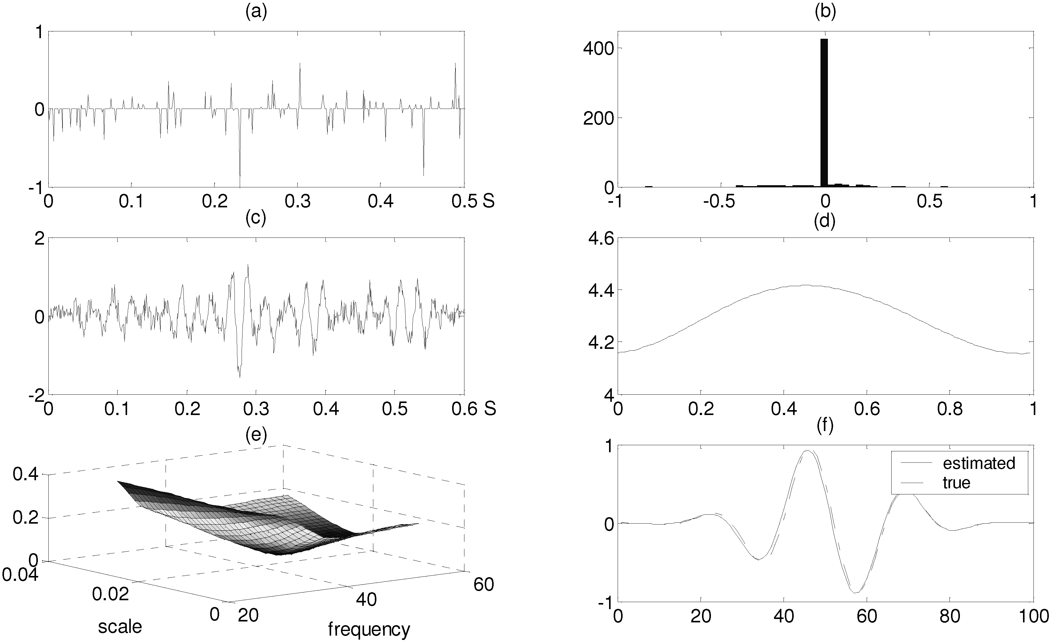
6.1. Simulation Results

We build a synthetic trace of length over 500 by convolving a super-Gaussian reflectivity with a wavelet defined by equation (2), plus additive white noise. Figure 4 plots the result of a simulation experiment. The reflectivity is simulated by a white process with GGD distribution, the true and estimated parameters are shown in table 6 respectively.
Table 6. Simulation.
σ f φ M ν λ SNR
True parameter 0.02 s 40.3 H z 0.4103 π 15 0.9 0.28 6 d B
Estimated parameter 0.02 s 39.875 H z 0.4544 π
Figure 4. (a) Super-Gaussian reflectivity sequence. (b) Reflectivity histogram. (c) Noisy seismic trace. (d) The kurtosis value of the rotated trace versus the rotation angle (the angle is represented as the multiple of π). (e) Cost surface. (f) Wavelet.
Entropy 12 00014 g004
Table 6 shows that the estimated quantities σ, f and φ are very close to their true values with small errors. This demonstrates that: (1) our method can work well over short time series, but the general CM method cannot; (2) our method has both strong anti-noise performance and high accuracy. Moreover, our method has low computational costs.

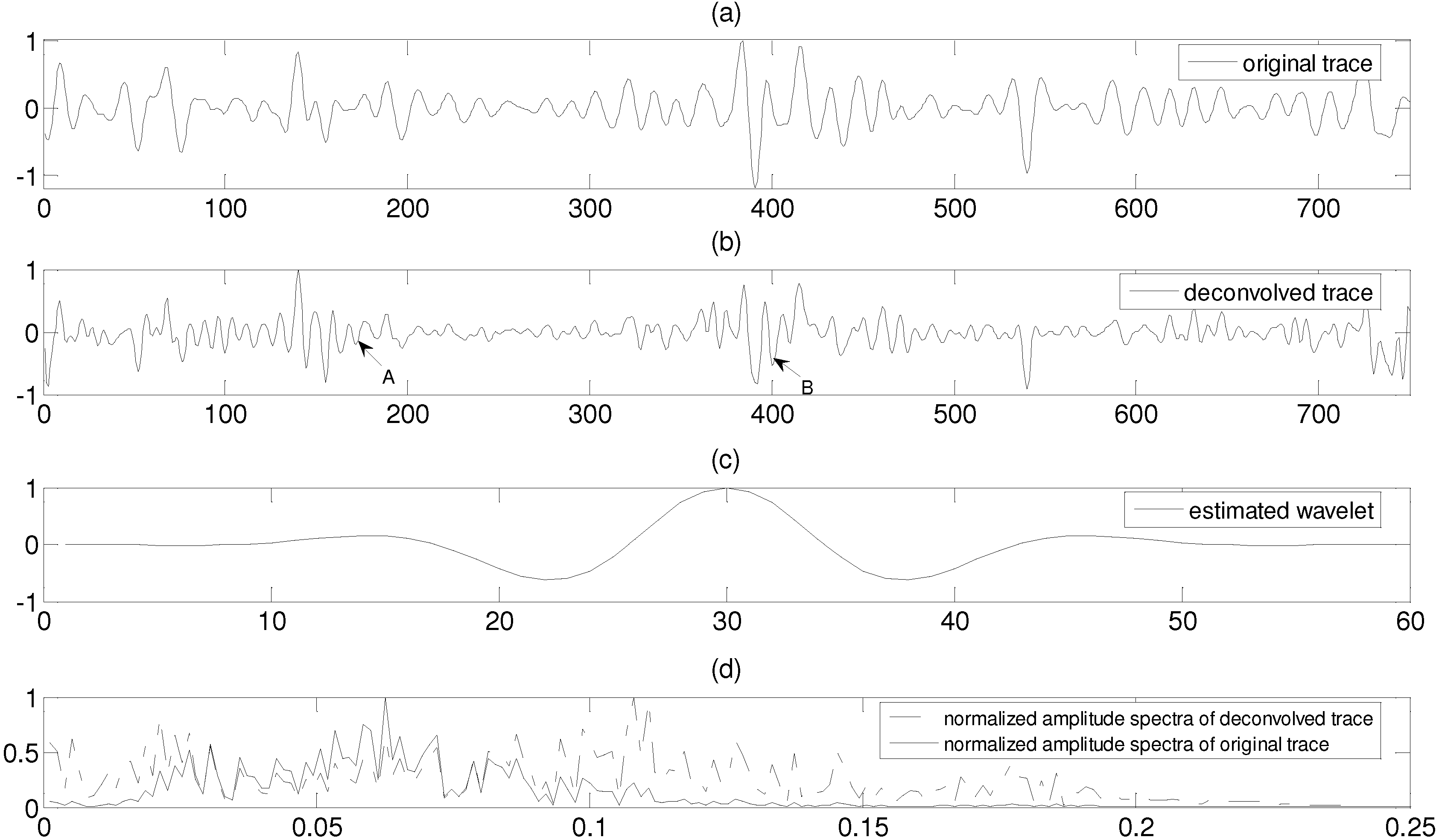
6.2. Real-data Experiment

Here, we consider real seismic trace with about 800 samples acquired from the Changqing oil field in China. It is noteworthy that the Wiener filter can achieve an optimum trade-off solution between deconvolution quality and noise amplification [6], so we find the seismic wavelet by our method and then improve the resolution of the seismic trace with the Wiener filter. The results are shown in Figure 5 where: (a) is original seismic trace, (b) denotes the deconvolved one, (c) is the estimated seismic wavelet, and (d) are amplitude spectrum of (a) and (b) respectively.
Let us compare (a) and (b). The seismic reflectors, labeled A, B in (b), are identified, but this cannot be done in (a) because of its poor resolution. Now let us compare them in frequency domain. Trace (d) shows that the amplitude spectrum of (b) is broader than (a). These show that the resolution of (b) is obviously high than (a).
Figure 5. Real-data experiment.
Entropy 12 00014 g005

7. Conclusions

In this paper, we have proposed a new approach based on the MSMG model for estimating seismic wavelets. We compared the performance using HOS derived from the MSMG model with that of the same one estimated directly from the recorded seismic trace. The method has been applied to synthetic and real traces. Simulation and real-data experiment have shown the ability of our approach in the presence of low Signal-to-Noise Ratio and the traces without a large amount of data available. We only give an application of our method for enhancing the resolution of seismic trace. In fact, it can be used any field where seismic wavelets must be estimated from seismic data, such as seismic trace inversion, Q estimated with WEPIF method, etc.

Acknowledgements

This work was supported by the NSFC (No. 40730424, and No. 40674074), and the HTRDPC (No. 2006AA09A102), and NSTMP (2008ZX05023-005-005). We thank the referees for their comments and criticisms that helped improve the paper.

References

  1. Robinson, E.A.; Treitel, S. Geophysical Signal Analysis; Prentice-Hall: Englewood Cliffs, NJ, USA, 1980; pp. 152–161. [Google Scholar]
  2. Peacock, K.I.; Treitel, S. Predictive deconvolution: theory and practice. Geophysics 1969, 43, 155–169. [Google Scholar]
  3. Larue, A.; Mars, J.I.; Jutten, C. Frequency-domain blind deconvolution based on mutual information rate. IEEE T. Signal Proces. 2006, 54, 1771–1781. [Google Scholar] [CrossRef]
  4. Larue, A.; Pham, D.T. Comparison of Supergaussianity and Whiteness Assumptions for Blind Deconvolution in Noisy Context. In Proceedings of the EUSIPCO 2006 Conference, Florence, Italy, September 4–9, 2006.
  5. Pham, D.T. Generalized mutual information approach to multi-channel blind deconvolution. Signal Process. 2007, 87, 2045–2060. [Google Scholar] [CrossRef]
  6. van der Baan, M.; Pham, D.T. Robust wavelet estimation and blind deconvolution of noisy surface seismics. Geophysics 2008, 73, 37–46. [Google Scholar]
  7. Nsiri, B.; Chonavel, T.; Boucher, J.-M.; Nouzé, H. Blind submarine seismic deconvolution for long source wavelets. IEEE J. Oceanic Eng. 2007, 32, 729–743. [Google Scholar] [CrossRef]
  8. Rosec, O.; Boucher, J.-M.; Nsiri, B.; Chonavel, T. Blind marine seismic deconvolution using statistical MCMC methods. IEEE J. Oceanic Eng. 2003, 28, 502–512. [Google Scholar] [CrossRef]
  9. Cheng, Q.; Chen, R.; Li, T.-H. Simultaneous wavelet estimation and deconvolution of reflection seismic signals. IEEE T. Geosci. Remote 1996, 34, 377–384. [Google Scholar] [CrossRef]
  10. Veils, D.R.; Ulrych, T.J. Simulated annealing wavelet estimation via fourth-order cumulant matching. Geophysics 1996, 61, 1939–1948. [Google Scholar] [CrossRef]
  11. Gao, J.-H.; Yang, S.-L.; Wang, D.-X. Q Factor Estimation Using Instantaneous Frequency at Envelope Peak of Seismic Signal. In Presented at the 79th Annual Meeting and International Exposition of the Society of Exploration Geophysicists, Houston, TX, USA, October 25–30, 2009.
  12. van der Baan, M. Time-varying wavelet estimation and deconvolution by Kurtosis maximization. Geophysics 2008, 73, v11–v18. [Google Scholar] [CrossRef]
  13. Hyvarinen, A.; Karhunen, J.; Oja, E. Independent Component Analysis; John Wiley & Sons Inc: New York, NY, USA, 2001. [Google Scholar]
  14. Bartlett, S.M. An Introduction to Stochastic Processes; Cambridge University Press: London, UK, 1955. [Google Scholar]
  15. Brillinger, D.R.; Rosenblatt, M. Computation and Interpretation of kth-order Spectra; Hams, B., Ed.; Spectral Analysis of Time Series; Wiley: New York, NY, USA, 1967; pp. 189–232. [Google Scholar]
  16. Øigard, T.A.; Hanssen, A.; Hansen, R.E.; Godtliebsen, F. EM-estimation and modeling of heavy-tailed processes with the multivariate normal inverse gaussian distribution. Signal Process. 2005, 85, 1655–1673. [Google Scholar] [CrossRef]
  17. Øigard, T.A.; Hanssen, A. The Multivariate Normal Inverse Gaussian Heavy-Tailed Distribution: Simulation and Estimation. Int. Conf. Acoust. Spee. 2002, 2, 1489–1492. [Google Scholar]
  18. Alecu, T.I.; Voloshynovskiy, S.; Pun, T. The gaussian transform of distributions: Definition, computation and application. IEEE T. Signal Proces. 2006, 54, 2976–2985. [Google Scholar] [CrossRef]
  19. Shiryayev, A.N. Probability; Springer-Verlag: New York, NY, USA, 1984. [Google Scholar]

Appendix

A. Calculating the Cumulant

Following from (18), let:
f ( z , ω ) = g Z ( z ) exp ( 1 2 z ω T Γ ω )
I n = 0 z n f ( z , ω ) d z
We have:
I n ω i = ( k = 1 N Γ i k ω k ) I n + 1
Using (19), we have:
Ψ y ( ω ) ω i = k = 1 N Γ i k ω k I 1 I 0 σ n 2 ω i
2 Ψ y ( ω ) ω i ω j = Γ i j I 1 I 0 + ( k = 1 N Γ i k ω k ) ( k = 1 N Γ j k ω k ) ( I 2 I 0 I 1 2 I 0 2 ) σ n 2 δ i j
3 Ψ y ( ω ) ω i ω j ω s = Γ i j ( k = 1 N Γ s k ω k ) ( I 2 I 0 I 1 2 I 0 2 ) + Γ i s ( k = 1 N Γ j k ω k ) ( I 2 I 0 I 1 2 I 0 2 ) + Γ j s ( k = 1 N Γ i k ω k ) ( I 2 I 0 I 1 2 I 0 2 ) ( k = 1 N Γ i k ω k ) ( k = 1 N Γ j k ω k ) ( k = 1 N Γ s k ω k ) [ I 3 I 0 I 2 I 1 I 0 2 2 ( I 1 I 0 I 2 I 0 I 1 2 I 0 2 ) ] = [ Γ i j ( k = 1 N Γ s k ω k ) + Γ i s ( k = 1 N Γ j k ω k ) + Γ j s ( k = 1 N Γ i k ω k ) ] ( I 2 I 0 I 1 2 I 0 2 ) ( k = 1 N Γ i k ω k ) ( k = 1 N Γ j k ω k ) ( k = 1 N Γ s k ω k ) ( I 3 I 0 3 I 1 I 2 I 0 2 + 2 I 1 3 I 0 3 )
4 Ψ y ( ω ) ω i ω j ω s ω t = ( Γ i j Γ s t + Γ i s Γ j t + Γ j s Γ i t ) ( I 2 I 0 I 1 2 I 0 2 ) [ Γ i j ( k = 1 N Γ s k ω k ) ( k = 1 N Γ t k ω k ) + Γ i s ( k = 1 N Γ j k ω k ) ( k = 1 N Γ t k ω k ) + Γ j s ( k = 1 N Γ i k ω k ) ( k = 1 N Γ t k ω k ) + Γ i t ( k = 1 N Γ j k ω k ) ( k = 1 N Γ s k ω k ) + Γ j t ( k = 1 N Γ i k ω k ) ( k = 1 N Γ s k ω k ) + Γ s t ( k = 1 N Γ i k ω k ) ( k = 1 N Γ j k ω k ) ] ( I 3 I 0 3 I 1 I 2 I 0 2 + 2 I 1 3 I 0 3 ) ( k = 1 N Γ i k ω k ) ( k = 1 N Γ j k ω k ) ( k = 1 N Γ s k ω k ) ( k = 1 N Γ t k ω k ) D t ( I 0 , I 1 , I 2 , I 3 )
where:
D t ( I 0 , I 1 , I 2 , I 3 ) = ( k = 1 N Γ t k ω k ) 1 ω t ( I 3 I 0 3 I 1 I 2 I 0 2 + 2 I 1 3 I 0 3 )
5 Ψ y ( ω ) ω i ω j ω s ω t ω m = [ ( Γ i j Γ s t + Γ i s Γ j t + Γ j s Γ i t ) ( k = 1 N Γ m k ω k ) + Γ i j Γ s m ( k = 1 N Γ t k ω k ) + Γ i j Γ t m ( k = 1 N Γ s k ω k ) + Γ i s Γ j m ( k = 1 N Γ t k ω k ) + Γ i s Γ t m ( k = 1 N Γ j k ω k ) + Γ j s Γ i m ( k = 1 N Γ t k ω k ) + Γ j s Γ t m ( k = 1 N Γ i k ω k ) + Γ i t Γ j m ( k = 1 N Γ s k ω k ) + Γ i t Γ s m ( k = 1 N Γ j k ω k ) + Γ j t Γ i m ( k = 1 N Γ s k ω k ) + Γ j t Γ s m ( k = 1 N Γ i k ω k ) + Γ s t Γ i m ( k = 1 N Γ j k ω k ) + Γ s t Γ j m ( k = 1 N Γ i k ω k ) ] ( I 3 I 0 3 I 1 I 2 I 0 2 + 2 I 1 3 I 0 3 ) + [ Γ i j ( k = 1 N Γ s k ω k ) ( k = 1 N Γ t k ω k ) + Γ i s ( k = 1 N Γ j k ω k ) ( k = 1 N Γ t k ω k ) + Γ j s ( k = 1 N Γ i k ω k ) ( k = 1 N Γ t k ω k ) + Γ i t ( k = 1 N Γ j k ω k ) ( k = 1 N Γ s k ω k ) + Γ j t ( k = 1 N Γ i k ω k ) ( k = 1 N Γ s k ω k ) + Γ s t ( k = 1 N Γ i k ω k ) ( k = 1 N Γ j k ω k ) ] ( k = 1 N Γ m k ω k ) D m ( I 0 , I 1 , I 2 , I 3 ) ω m [ ( k = 1 N Γ i k ω k ) ( k = 1 N Γ j k ω k ) ( k = 1 N Γ s k ω k ) ( k = 1 N Γ t k ω k ) D t ( I 0 , I 1 , I 2 , I 3 ) ]
6 Ψ y ( ω ) ω i ω j ω s ω t ω m ω n = ( Γ i j Γ s t Γ m n + Γ i s Γ j t Γ m n + Γ j s Γ i t Γ m n + Γ i j Γ s m Γ t n + Γ i j Γ t m Γ s n + Γ i s Γ j m Γ t n + Γ i s Γ t m Γ j n + Γ j s Γ i m Γ t k + Γ j s Γ t m Γ i n + Γ i t Γ j m Γ s n + Γ s t Γ j m Γ i n + Γ s t Γ i m Γ j n + Γ j t Γ s m Γ i n + Γ j t Γ i m Γ s n + Γ i t Γ s m Γ j n ) ( I 3 I 0 3 I 1 I 2 I 0 2 + 2 I 1 3 I 0 3 ) + [ ( Γ i j Γ s t + Γ i s Γ j t + Γ j s Γ i t ) ( k = 1 N Γ m k ω k ) + Γ i j Γ s m ( k = 1 N Γ t k ω k ) + Γ i j Γ t m ( k = 1 N Γ s k ω k ) + Γ s t Γ j m ( k = 1 N Γ i k ω k ) + Γ s t Γ j m ( k = 1 N Γ j k ω k ) + Γ j s Γ t m ( k = 1 N Γ i k ω k ) + Γ j t Γ i m ( k = 1 N Γ s k ω k ) + Γ i t Γ s m ( k = 1 N Γ j k ω k ) + Γ i t Γ j m ( k = 1 N Γ s k ω k ) + Γ j s Γ t m ( k = 1 N Γ i k ω k ) + Γ j t Γ i m ( k = 1 N Γ t k ω k ) + Γ i s Γ t m ( k = 1 N Γ j k ω k ) + Γ i s Γ j m ( k = 1 N Γ t k ω k ) ] ( k = 1 N Γ n k ω k ) D n ( I 0 , I 1 , I 2 , I 3 ) + Ψ y ( ω ) ω n { [ Γ i j ( k = 1 N Γ s k ω k ) ( k = 1 N Γ t k ω k ) ) + Γ i s ( k = 1 N Γ j k ω k ) ( k = 1 N Γ t k ω k ) + Γ j s ( k = 1 N Γ i k ω k ) ( k = 1 N Γ t k ω k ) + Γ i t ( k = 1 N Γ j k ω k ) ( k = 1 N Γ s k ω k ) + Γ j t ( k = 1 N Γ i k ω k ) ( k = 1 N Γ s k ω k ) + Γ s t ( k = 1 N Γ i k ω k ) ( k = 1 N Γ j k ω k ) ] ( k = 1 N Γ m k ω k ) D m ( I 0 , I 1 , I 2 , I 3 ) } 2 ω m ω n [ ( k = 1 N Γ i k ω k ) ( k = 1 N Γ j k ω k ) ( k = 1 N Γ s k ω k ) ( k = 1 N Γ t k ω k ) D t ( I 0 , I 1 , I 2 , I 3 ) ]
To calculate the cumulants, we need compute the following statistics:
I 1 I 0 | ω = 0 = E ( Z )
I 2 I 0 ( I 1 I 0 ) 2 | ω = 0 = E ( Z 2 ) [ E ( Z ) ] 2 = var ( Z )
I 3 I 0 3 I 1 I 2 I 0 2 + 2 ( I 1 I 0 ) 3 | ω = 0 = E ( Z 3 ) 3 E ( Z ) E ( Z 2 ) + 2 E 3 ( Z )
Hence, we have:
c u m ( 2 ) ( y i , y j ) = 2 Ψ y ( ω ) ω i ω j | ω = 0 = Γ i j E ( Z ) + σ n 2 δ i j
c u m ( 3 ) ( y i , y j , y s ) = j 3 Ψ y ( ω ) ω i ω j ω s | ω = 0 = 0
c u m ( 4 ) ( y i , y j , y s , y t ) = 4 Ψ y ( ω ) ω i ω j ω s ω t | ω = 0 = ( Γ i j Γ s t + Γ i s Γ j t + Γ j s Γ i t ) var ( Z )
c u m ( 5 ) ( y i , y j , y s , y t , y m ) = j 5 Ψ y ( ω ) ω i ω j ω s ω t ω m | ω = 0 = 0
c u m ( 6 ) ( y i , y j , y s , y t , y m , y n ) = 6 Ψ y ( ω ) ω i ω j ω s ω t ω m ω n | ω = 0 = ( Γ i j Γ s t Γ m n + Γ i s Γ j t Γ m n + Γ j s Γ i t Γ m n + Γ i j Γ s m Γ t n + Γ i j Γ t m Γ s n + Γ i s Γ j m Γ t n + Γ i s Γ t m Γ j n + Γ j s Γ i m Γ t k + Γ j s Γ t m Γ i n + Γ i t Γ j m Γ s n + Γ s t Γ j m Γ i n + Γ s t Γ i m Γ j n + Γ j t Γ s m Γ i n + Γ j t Γ i m Γ s n + Γ i t Γ s m Γ j n ) [ E ( Z 3 ) 3 E ( Z ) E ( Z 2 ) + 2 E 3 ( Z ) ]

B. Calculating the Ratios of cy(k)1, τ2, …, τk-1) to cyk for Fourth-order and Sixth-order

Since Γ RN×N is a positive definite symmetric matrix, we denote the its diagonal element Γii = Γ0 (i = 1,2, …, N), thus, using (A6), we have:
c y 2 = c u m ( 2 ) ( y i , y i ) = Γ 0 E ( z ) + σ n 2
c y 4 = c u m ( 4 ) ( y i , y i , y i , y i ) = 3 Γ 0 2 var ( z )
c y 6 = c u m ( 6 ) ( y i , y i , y i , y i , y i , y i ) = 15 Γ 0 3 [ E ( z 3 ) 3 E ( z ) E ( z 2 ) + 2 E 3 ( z ) ]
Using (9) and (A6c), we have:
r y ( 4 ) ( y i , y j , y s , y t ) = c u m ( 4 ) ( y i , y j , y s , y t ) c y 4 = ( Γ i j Γ s t + Γ i s Γ j t + Γ j s Γ i t ) E 2 ( Z ) 3 Γ 0 2 E 2 ( Z )
Noting that RS is equal to E(Z)Γ, and the clean seismic data is a zero-mean discrete stationary random process, we have:
Γ i j E ( Z ) Γ 0 E ( Z ) = R s ( j i ) R s ( 0 ) = ρ s ( j i )
Using (B2) and (B3), we have:
r y ( 4 ) ( y i , y j , y s , y t ) = 1 3 [ ρ s ( j i ) ρ s ( t s ) + ρ s ( s i ) ρ s ( t j ) + ρ s ( j s ) ρ s ( t i ) ]
Similarly, combined with (9), (A6e), (B1c) and (B3), the following equation holds:
r y ( 6 ) ( y i , y j , y s , y t , y m , y n ) = ( Γ i j Γ s t Γ m n + Γ i s Γ j t Γ m n + Γ j s Γ i t Γ m n + Γ i j Γ s m Γ t n + Γ i j Γ t m Γ s n + Γ i s Γ j m Γ t n + Γ i s Γ t m Γ j n + Γ j s Γ i m Γ t n + Γ j s Γ t m Γ i n + Γ i t Γ j m Γ s n + Γ s t Γ j m Γ i n + Γ s t Γ i m Γ j n + Γ j t Γ s m Γ i n + Γ j t Γ i m Γ s n + Γ i t Γ s m Γ j n ) E 3 ( Z ) 15 Γ 0 3 E 3 ( Z ) = [ ρ s ( j i ) ρ s ( t s ) ρ s ( n m ) + ρ s ( s i ) ρ s ( t j ) ρ s ( m n ) + ρ s ( j s ) ρ s ( t i ) ρ s ( m n ) + ρ s ( j i ) ρ s ( m s ) ρ s ( n t ) + ρ s ( j i ) ρ s ( t m ) ρ s ( n s ) + ρ s ( s i ) ρ s ( m j ) ρ s ( n t ) + ρ s ( s i ) ρ s ( t m ) ρ s ( n j ) + ρ s ( s j ) ρ s ( m i ) ρ s ( n t ) + ρ s ( j s ) ρ s ( m t ) ρ s ( n i ) + ρ s ( t i ) ρ s ( m j ) ρ s ( n s ) + ρ s ( s t ) ρ s ( m j ) ρ s ( n i ) + ρ s ( t s ) ρ s ( m i ) ρ s ( n j ) + ρ s ( t j ) ρ s ( m s ) ρ s ( n i ) + ρ s ( t j ) ρ s ( m i ) ρ s ( n s ) + ρ s ( t i ) ρ s ( m s ) ρ s ( n j ) ] / 15

