1. Introduction
In recent years more attention has been paid to thermodynamics and statistical mechanics in the atmospheric sciences and other fields studying many-body systems like oceanography. In addition to the large number of journal articles [
1,
2,
3,
4,
5,
6,
7,
8,
9,
10], several monographs have been published in succession [
11,
12,
13].
Early in the 1940s Eady pointed out the rather formidable task facing theoretical meteorology – that of discovering the nature of and determining quantitatively all the forecastable regularities of a “permanently unstable” (i.e., permanently turbulent) system, and firmly believed that “we can be certain that these regularities are necessarily statistical and to this extent our technique must resemble statistical mechanics” [
14].
Entropy flow is a core concept in non-equilibrium thermodynamics just as entropy is in classical thermodynamics and statistical physics. According to the second law of thermodynamics, an isolated system will evolve spontaneously into the equilibrium with maximum entropy in which the order of the system is a minimum [
15,
16]. As a result, negative entropy is very important for an open system to remain far from equilibrium, which is also true in biological systems as reflected in the statement that life’s existence depends on its continuous gain of “negentropy” from its surroundings [
17,
18].
The atmosphere has been likened to a giant thermodynamic engine in which disorganized heat energy is transformed into the organized kinetic energy of the winds. The general circulation of the atmosphere can be regarded as simply being driven by temperature differences between the polar and equatorial regions [
19].
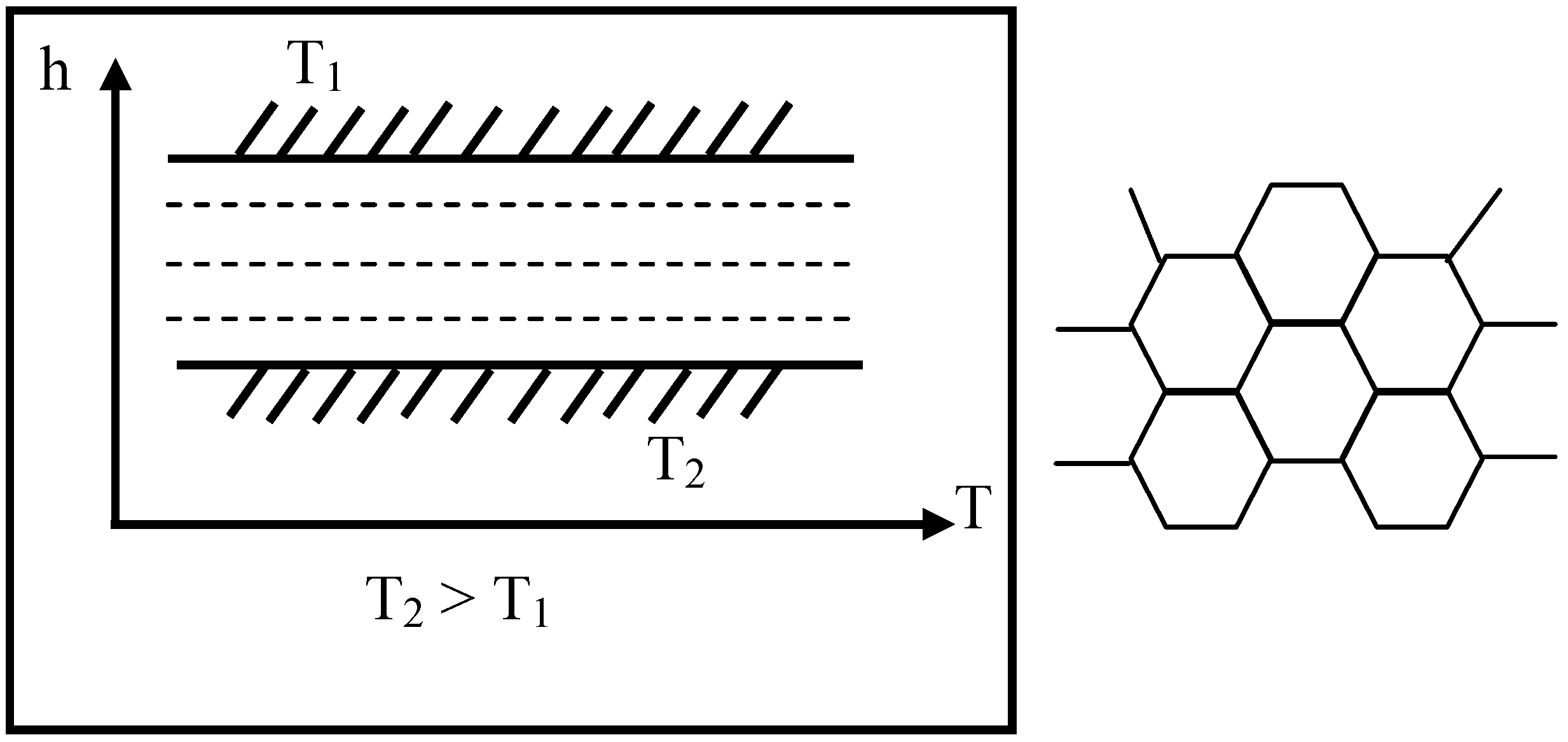
Figure 1.
The schematic diagram for Bénard convection as the prototype of self-organization, showing that the temperature difference (T2-T1) reaching a certain critical value (threshold) will cause the macro-scale convection to occur within the system. Note that the temperature difference (T2-T1) > 0 will lead the entropy exchange < 0, meaning that the system gains “negative entropy”. See text for details.
The classical Bénard convective system is driven by a vertical temperature difference, and well-organized hexagonal convective cells abruptly form within a thin layer of fluid originally at rest once the temperature difference reaches a certain critical value (see
Figure 1). This system demonstrates that systems which get heat at a higher temperature and lose heat at a lower temperature will gain “negentropy” from its surroundings. The troposphere experiences a double negative entropy flow process, in the horizontal and vertical, since it gets heat at the tropics and the surface with higher temperature and loses heat at the poles and the tropopause which have lower temperatures, respectively. This suggests a possible explanation for the variety of weather in the troposphere.
In this paper, our starting point is based on the argument that negative entropy flow might drive a system to a state further apart from equilibrium in which its entropy reaches the maximum. It follows that negative entropy flow is important in the sense that it will favor the development or organization of a system such as storm.
In the field of the atmospheric sciences the theory of entropy has been mostly applied to global-scale and/or climatic investigations using the general circulation models or climatic models. For example, the entropy budget of the atmosphere as a whole has been estimated through the entropy balance equations and, the global climate system has been examined using the principle of minimum entropy exchange [
20,
21,
22]. A number of more recent climate studies involve also entropy-flux and entropy production [
23,
24,
25]. In addition to global-scale researches, a cloud ensemble model is used to study the entropy budget as well [
26,
27].
With respect to applications of entropy theory to numerical prediction, we would like to mention again the research in which the authors reviewed atmospheric systems in light of non-linear non-equilibrium thermodynamics and reached a series of results, including: numerical simulation of atmospheric circulation improved dramatically when the second law of thermodynamics is incorporated into a global spectrum model [
10]; and, the forecast accuracy of a meso-scale numerical weather prediction model is noticeably enhanced by introducing a physics-based diffusion scheme [
6,
7]. Besides, precursors of cyclogenesis over a specific region have been investigated using the spatial distribution of the moist entropy although the physical connotation of this entropy in their context should be, in nature, different from that of the classical thermodynamic entropy [
28].
The purpose of this paper is to derive entropy flow equations for calculating the instantaneous entropy flow field and to discuss the relationship of entropy flow with the life cycle of an atmospheric system - a tropical storm (TS) - with the aim of revealing the dependence of the growth of the system on negative entropy flow. The TS selected for this study is tropical storm Bilis, hereafter called TS Bilis, which struck land on Fujian, China in 2006 and was the worst such disaster in Eastern China in the last ten years, as it caused the most deaths. The entropy flow computations for the various stages of its life-cycle are based on the National Centers for Environmental Prediction/National Center for Atmospheric Research (NCEP/NCAR) 1°×1° (latitude-longitude) resolution reanalysis data [
29].
1.1 Background
The second law of thermodynamics can be expressed in terms of the entropy balance equation provided local equilibrium is assumed [
16]. The entropy change in an open system usually consists of two parts: one is entropy flow that is caused by the exchange of entropy in the system with its surroundings and the values of entropy flow can be either negative or positive; and, the other is positive definite entropy production caused by irreversible processes within the system.
The Gibbs relation under the assumption of local equilibrium [
30] can be written in terms of the change of entropy per unit mass, s, with time
where
and
The three individual derivatives in the right-hand side of equation 1 can be found through the first law of thermodynamics, the continuity equation and the component balance equation. The first law can be written as
where
and
can be related to
via the continuity equation
where
and, the component balance equation can be written as
Substituting for the three individual time derivatives in the right-hand side of equation 1 by equations 4, 5 and 7 and turning the derivation of entropy into the local derivative, we have
where
is called entropy production while the “div” term is the entropy flow.
Usually the contribution of
to the entropy flow in the atmosphere is neglectable compared with
while the diffusive flow
for component
k can be defined as [
31]
In this paper the component of liquid water has been omitted owing to the liquid water content (about 5 gm-
3 on the average over the tropics) being much less than the density of either vapor or dry air [
32,
33] and only two components are therefore taken into account, that is, vapor and dry air. Usually the velocity
for vapor is assumed to be the same as
for dry air so that
in this case. As a consequence, the entropy
s per unit mass consists accordingly of
sq for vapor and
sd for dry air with all the corresponding entropy constants,
sq0 and
sd0, to vapor and dry air, respectively, set to zero so that
The formulas above are derived based on Cartesian coordinates but the NCEP/NCAR reanalysis data used in this paper are on constant pressure layers, so it is necessary to transform the expression of entropy flow into that in the p-coordinates
Equation 12 is the fundamental formula for diagnosing entropy flow employed in this paper.
1.2 Case Description
TS Bilis struck land at Fujian, China on 14 July 2006, and caused direct economic losses of US$5.1 billion, 654 deaths and 208 missing persons. TS Bilis formed in the afternoon on 9 July 2006, developed and reached maturity on 0000 UTC 12 July. Its prime was from 0000 UTC 13 July to 0000 UTC 14 July, after which it began to decay.
The entropy flows for the different evolutionary stages of this storm are examined. These flows are evaluated using equation 12 and the NCEP/NCAR 1°×1° (latitude-longitude) resolution reanalysis data [
29].
2. Results and Discussion
Changes in the entropy flow at the near surface 850 hPa layer are examined initially and related to the evolution of TS Bilis. A more detailed discussion about the dependence of the growth of the three-dimensional storm as a thermodynamic system on the negative entropy flow for its whole life-cycle is made in the last portion of this paper.
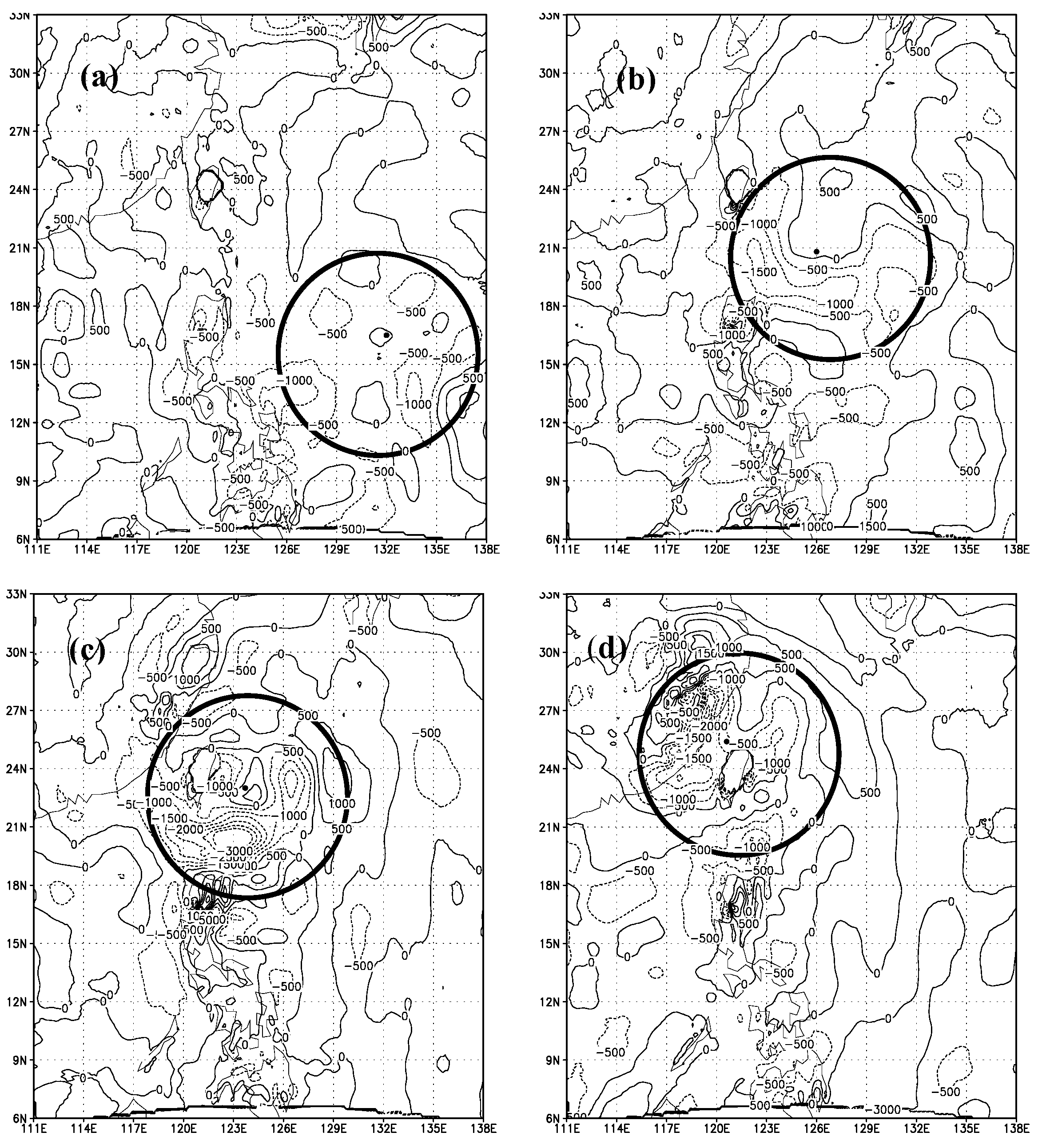
Figure 2.
Entropy flow fields at 850 hPa in the different evolution stages of TS Bilis (2006): (a) genesis (0600 UTC 10 July), (b) development (0000 UTC 12 July), (c) maturity (0000 UTC 13 July), and (d) decay (0000 UTC 14 July). The contour interval is 0.5×10³ JK-1s-1, and the circle is centered on the storm and indicates its extent.
Representative times for TS Bilis genesis or its initial stage, development, maturity and decay stages are determined as 0600 UTC 10, 0000 UTC 12, 0000 UTC 13 and 0000 UTC 14 July, respectively.
In the initial stage [
Figure 2(a)], negative entropy flow dominates the circled region, with a maximum negative entropy flow of about -1×10
3 JK
–1s
-1. TS Bilis develops with time and the area with negative entropy flow greater than -1×10
3 JK
–1s
-1 within the region expands with the maximum negative entropy flow strengthening to around –1.5×10
3 JK
–1s
-1 as seen at 0000 UTC 12 July [
Figure 2(b)]. TS Bilis then enters its mature stage with a central pressure below 980 hPa until 0000 UTC 13 July when the negative entropy flow around the storm center and in its neighborhood reaches a maximum negative entropy flow greater than -3×10
3 JK
–1s
-1 [
Figure 2 (c)]. From 0600 UTC 13 to 0000 UTC 14 July TS Bilis is at its maximum with a central pressure down to 975 hPa. At 0000 UTC 14 July it starts to decay and the corresponding negative entropy flow is decreased [
Figure 2 (d)].
Next the longitude- and latitude-vertical cross sections of entropy flow through the storm center will be analyzed in order to further understand the dependence of the growth of the storm on negative entropy flow.
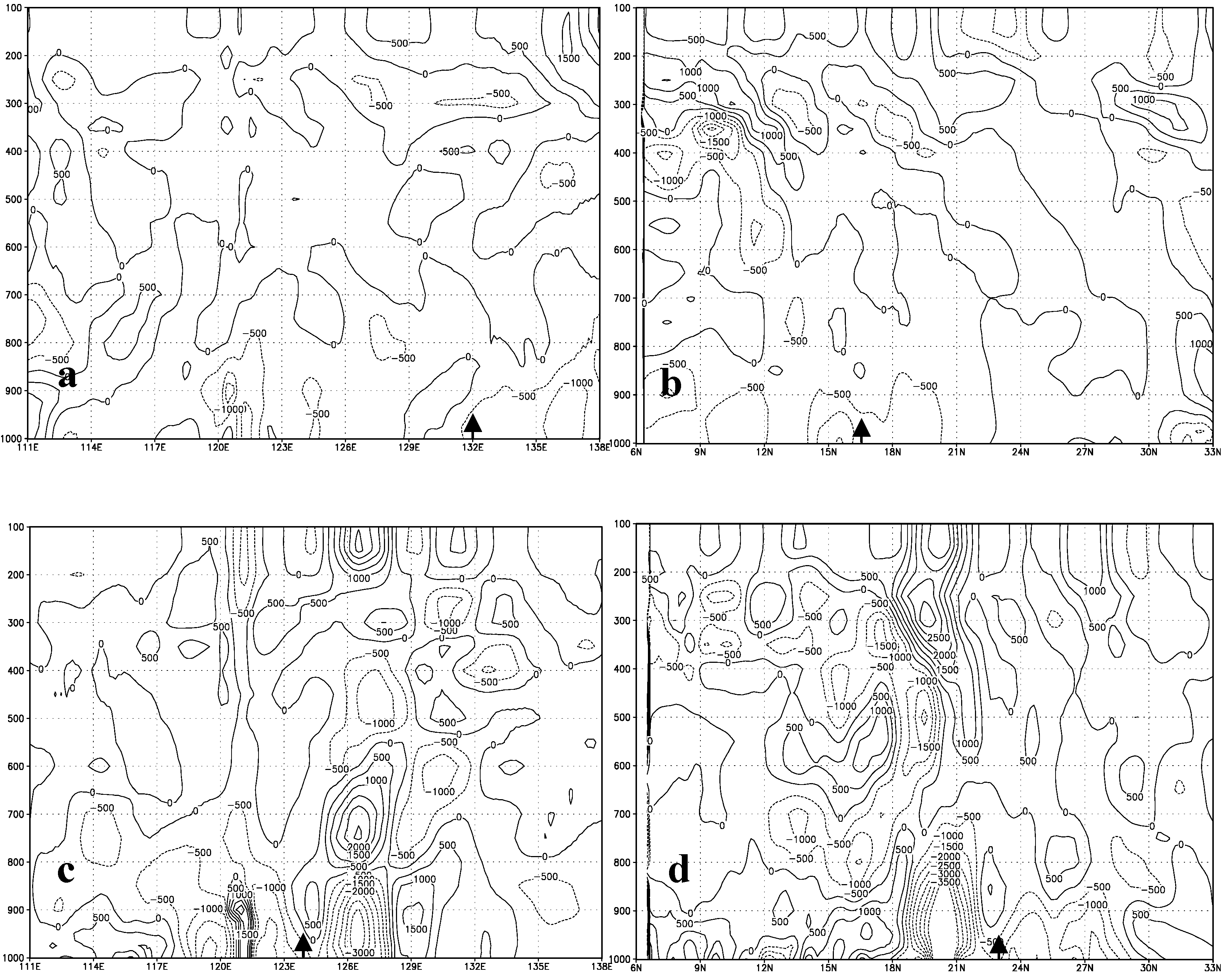
Figure 3.
The pressure-longitudinal (a)/(c) and pressure-latitudinal (b)/(d) cross sections of entropy flow through TS Bilis’ centre at 0600 UTC 10/0000 UTC 13 July, respectively. The contour interval is 0.5×10³ J K-1 s-1, and the black triangles indicate the respective positions of the storm center at the surface.
Figure 3 shows the cross sections of entropy flow at 0600 UTC 10 and 0000 UTC 13 July for the genesis and mature stages of TS Bilis, respectively.
During the genesis stage negative entropy flow is weak, especially in the lower troposphere [
Figure 3(a)-
Figure 3(b)]. It gradually becomes stronger and expands toward the upper levels with the rapid development of the storm. In the development stage areas of negative entropy flow have reached 300
hPa in the longitudinal cross section, and in the mature stage these regions have almost penetrated the whole troposphere up to 200 hPa or higher [
Figure 3(c)-
Figure 3(d)]. Such vertical penetration of negative entropy flow continues until 0000 UTC 14 July when TS Bilis starts to decay with a drop of 5 ms
-1 in the maximum surface wind and rise by 5 hPa in the central pressure within 6 h. This suggests that changes in the entropy flow should be an indication of changes in the intensity of a storm.
Finally we will examine the total entropy flow (TEF) of the storm. The TEF of a storm system is defined by summing the entropy flow over every grid point within a system at a constant pressure layer and then over every layer, leading TEF to be a single number standing for the intensity of entropy flow for the system at any given time. Entropy flow of a three-dimensional storm system through its boundary that is a curved surface
A can be worked out by integrating the divergence of the entropy flow vector
over the whole system volume
V (the summing over all the grid points encompassed by the curved surface is the discrete version of the integration) based on the well-known Gaussian formula [
34]
The integrand in the right hand side of equation 7 is just the divergence of the entropy flow vector in this case.
In this paper the approximate total entropy flow is calculated on each pressure layer, by summing over all grid points within a circle centered on the storm’s center with a radius of six degrees (thus the horizontal boundaries of the storm are defined), and then summed over all layers (thus the top and bottom pressure layer are treated as its vertical boundaries).
Figure 4.
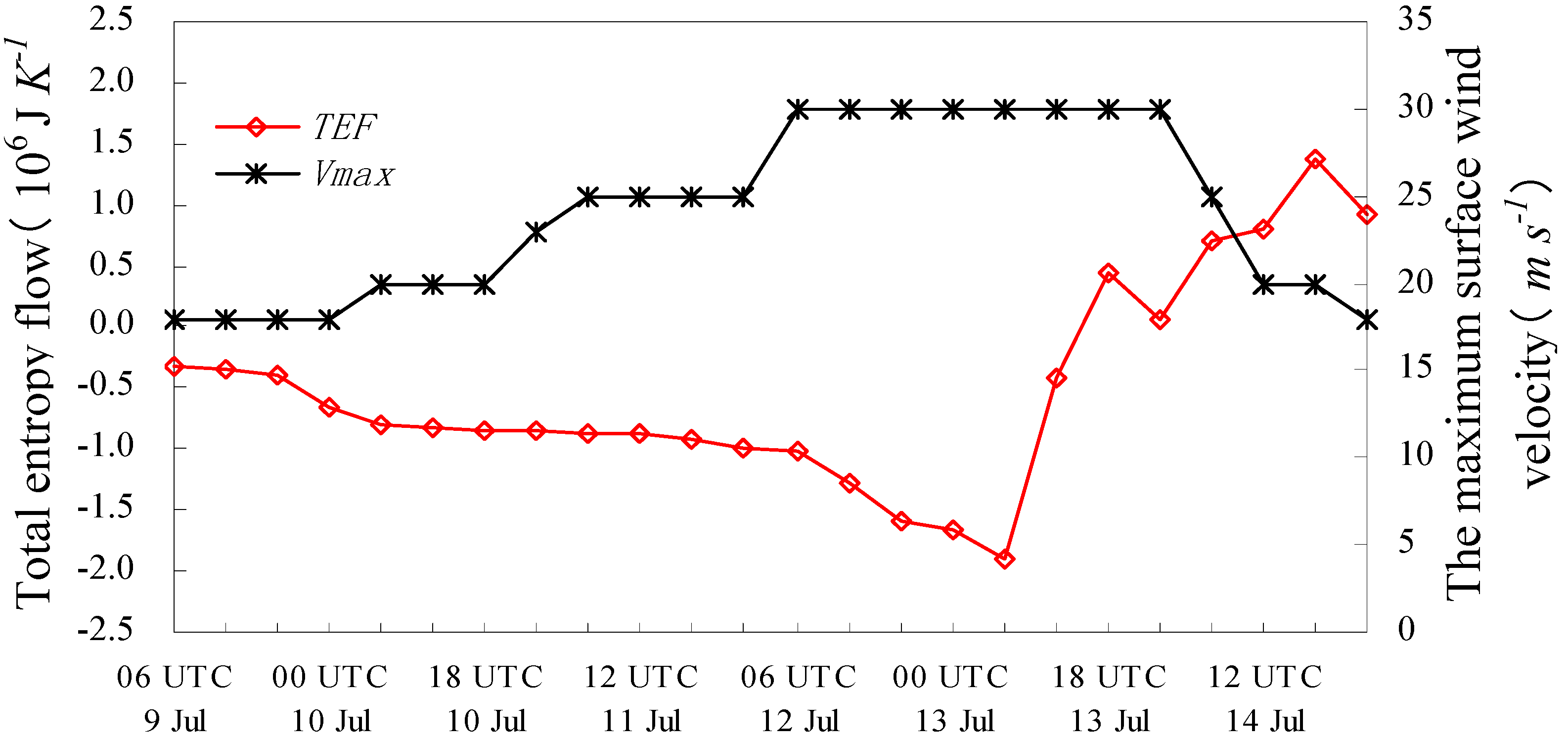
The evolution of total entropy flow (TEF) for TS Bilis in 6 h timesteps, with changes in the maximum surface wind velocity (Vmax) as a reference.
Figure 4.
The evolution of total entropy flow (TEF) for TS Bilis in 6 h timesteps, with changes in the maximum surface wind velocity (Vmax) as a reference.
In view of that the evolution of the maximum surface wind of TS Bilis falls into three stages: (1) intensification before 0600 UTC 12 July during which the maximum wind monotonically increases from 18 ms
-1; (2) maintenance from 0600 UTC 12 to 0000 UTC 14 July during which the maximum wind maintains its maximum of 30 ms
-1, with a small drop in the central pressure from 980 to 975 hPa at 0000 UTC 13 July; and, (3) decay from 0000 UTC 14 July during which the maximum wind continuously decreases from 30 ms
-1, the calculations will then be made correspondingly to these stages (
Figure 4). The results show that the total entropy flows around TS Bilis are negative and intensify monotonically during stage (1); in stage (2), where the maximum surface wind is kept at its maximum, the evolution of the TEF for the storm has a strong drop in the (negative) total entropy flow which then turns gradually to positive TEF; and, during stage (3) after 0000 UTC 14 July the total entropy flow around the storm and its neighborhood is positive. This implies that the growth of an atmospheric system may rely upon the negative entropy flow.
3. Conclusion
According to classical thermodynamics, the entropy of an isolated system will run to the maximum that corresponds to equilibrium in which no ordered structure forms. On the other hand, the nonlinear non-equilibrium thermodynamics points out that for an open system a negative entropy flow strong enough from its surroundings may drive the system to a state far from equilibrium so as to form dissipative structures, suggesting that negative entropy is something very important for structural creation and development in a thermodynamic system. However, the effect of entropy flow on the evolution of an atmospheric system is unknown.
This study reveals, via the entropy flow analysis of TS Bilis based on the entropy balance equation derived from the Gibbs relation and using NCEP/NCAR reanalysis data, that the entropy flow properties of this severe tropical storm are different in the different stages of its life-cycle and, especially that the growth of a severe atmospheric system may rely upon the negative entropy flow. As a result, entropy flow analysis might provide a powerful tool to understanding the mechanism responsible for the life cycle of an atmospheric system and associated weather events.
This is a preliminary case study and we intend to investigate a series of tropical storms and other vortices in the atmosphere. Only the generally accepted results reached in this field would potentially contribute to properly judging whether the entropy flow methodology can be generalized to the other relevant fields to investigate the life cycle of an ordered system, whether it is living or nonliving.


