2. Ecosystem phase space
The state of any complex system can be expressed in a multitude of ways. At the coarsest resolution, this might be specification of macro-properties such as temperature and pressure for gases. A more detailed description would give the trajectories of representative particles in a small region. The exact description would give the location and momentum of every particle. Of course the last description is precluded by the Heisenberg uncertainty principle.
The intermediate resolution description has proved to be extraordinarily useful in applications of quantum mechanics. Briefly, this is how the approach works. The uncertainty principle provides the theoretical basis for defining regions where particle properties can be assessed. These regions are simply discrete cells in a phase space. The size of the cells is determined by Heisenberg’s principle. This gives the cell size as a fraction of a six-dimensional phase space whose elements are the three components of position and three components of momentum. The fundamental cell size is given by h3 or h3/2 for BE and FD models, respectively, where h is Planck’s constant. Typically the number of cells in phase space greatly exceeds the number of particles in the gas.
The phase space concept, as just outlined, leads naturally to the concept of micro and macro states. The microstate description specifies the number of particles in each cell. Now the cells can be grouped by zones of approximately the same energy or some other appropriate macro-property. The distribution of particles in each zone is the macrostate description. Considering the large number of particles and cells or zones, it is clear that a given macrostate can be achieved by a large number of microstates. The macrostate(s) determined by the largest numbers of microstates is (are) the one(s) most likely to be observed at equilibrium.
The notion of phase space with associated micro and macrostates is quite general and has been applied with great effect in many disciplines other than quantum mechanics. Here I attempt to apply these ideas to ecosystems. The first step in constructing an ecosystems phase space is to specify the cell characteristics. But what to do since there is no biological uncertainty principle?
In order to address this question it is useful to begin with a review of Heisenberg’s uncertainty principle. An elementary form is
where ∆
p and ∆
x are momentum and position increments or observational uncertainties along the
x axis. Equation (1) is purposefully written as an inequality to emphasize the point that in a given experiment or set of observations, the product of increments often is larger than the Heisenberg fundamental limit
h. From the biological perspective (1) is just an allometric equation relating position and momentum with a scaling exponent of −1.
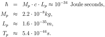
Can a biological counterpart of h be constructed? To answer this, recall that h was first introduced as the coefficient in Planck’s equation relating the energy ε of photons to their frequencies ν. Incidentally, that equation (ε = hν) is also an allometric equation with a scaling exponent of 1. The universal gravitation constant G, the speed of light c, and h define fundamental mass (Mp), length (Lp), and time (Tp) scales. See Gross (1989)and Wilczak (2001) for concise histories and insightful discussions about these scales.
Apparently analogous universal constants have yet to be identified for biological processes. Consequently, I attempt here to construct an
hE from appropriate mass, length, and time scales. Of all the allometric relations in biology, what are the ones most appropriate for ecosystems? Ginzburg and Golyvan (2004) state that the essential allometric equations for describing ecosystems are: Kleiber’s equation for metabolic rate
R, generation time
τ, and Damuth’s equation for the population density
D. The appropriate allometric equations are
Here
M is mass, and the
γ’s are normalization factors, or the ordinate intercepts on a log log plot. I specify their dimensions as [
M1/4L2/
T3], [
TM−1/4], and [
M3/4/
L2], respectively.
Equation (2) is consistent with the quarter-power scaling proposed by West et al. (1997). This specific scaling, along with the general issue of appropriateness of allometric equations in biology, are topics of lively discussion in the literature. Two recent papers illustrate some of the relevant issues. In an exhaustive re-analysis of earlier data, Dodds et al. (2001) rejected a quarter-power scaling of metabolic rate for animals in favor of a geometric scaling. They also disputed the theoretical justification for quarter-power scaling developed by West et al. (1997). On the other hand, Kaitaniems (2004) argued that much of the variability in estimates of scaling exponents are procedural artifacts. West and Brown (2005) have responded to Dodds et al. (2001) criticism of the theoretical basis of quarter-power scaling, but this is not likely to be the final word. In view of this, the use of quarter-power scaling here is not an endorsement; it is merely a convenient example scaling. The basic idea of an ecosystem uncertainty parameter or minimum phase space cell does not depend on a specific scaling, only on the presumption that a consistent scaling exists.
The dimensions of h are [ML2/T]. For the scaling argument used below Planck’s reduced constant, ħ = h/2π ≈ 10−34 Joule seconds is appropriate. Surely an ecosystem phase space cell should have the same dimensions. After all, life is based on fundamental physical and chemical processes taking place down to the quantum level.
An ecosystem uncertainty parameter
hE with dimensions [
ML2/
T] can be constructed from the
γ’s in (2). That is, select
α,
β, and
δ such that
has the dimensions of
h in (1). Straightforward algebra yields
At this point there is nothing to constrain the number of normalization parameters, or γ’s. A phase space can be built on any consistent choice. Indeed this situation parallels the history of statistical mechanics. The father of this discipline, Ludwig Boltzmann, did not even know of the uncertainty principle, he merely stipulated the existence of cells. It wasn’t until after the rise of quantum mechanics, decades after Boltzmann’s untimely death, that the precise specification of a phase space cell in a quantum gas was established.
As noted earlier,
h is the minimum of all possible scaling coefficients for (1). Similarly, we seek the minimum
hE. If this is to be a universal quantity characteristic of life, then it should be based on scales of the most fundamental of life forms, microbes. Of course time, space, and mass scales of microbes range over orders of magnitude. Moreover, microbial space scales are highly anisotropic, which is in distinct contrast to a quantum gas in the absence of an external field, and precise values are not yet available. Nevertheless estimates based on values reported in the literature for selected species are of interest. To avoid issues arising from spatial anisotropy, the spherical microbe
Staphylococus is a convenient choice. Typical scales appropriate for this organism, as reported by Doetsch and Cook (1973), are mass
Mm ≈ 10
−16kg, space
Lm ≈ 10
−6m, and
Tm ≈ 2 · 10
3s respectively. Then
Estimates of
hE based on other microbe scales reported by Doetsch and Cook (1973 varied from 10
−29 to 10
−32.
These values are surprisingly close to
ħ = 10
−34 Joule seconds, and thus merit comment. To this end, note that
ħ can also be expressed in terms of the product of the momentum and size of a Planck photon, the smallest possible photon. See Kirwan (2004) for a discussion of this point. As is well known photon momentum is simply
Mp ·
c where
is the speed of light. Thus
Comparison of the values in (6), with the microbal scales used in constructing (5), shows that Mm is 8 orders of magnitude smaller than Mp, Lm is over 29 orders of magnitude larger than Lp, and Tm is 47 orders of magnitude larger than Tp. Essentially ħ is small because the Planck length scale Lp is small. In contrast hE is small because Tm is large. Indeed it is large time scales that distinguish biological processes from typical quantum physical and chemical processes.
It was noted earlier that there are generally many more cells than particles in quantum phase space. Put another way, in a quantum gas at any given time there may be cells with no particles. The small value of
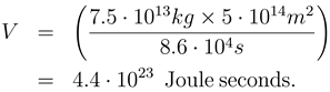
hE suggests this could be true for ecological phase space. An enlightening calculation is to estimate the number of cells for ecosystem earth. A conservative estimate of the size of this phase space is the biomass of earth times the surface area of the earth divided by an appropriate planetary time scale. Using one day as the time scale, this gives a phase space volume of
The number of cells is simply (7) divided by (5) or about 10
54 cells in ecosystem earth.
This calculation assumes ecosystem earth exists on a surface. Of course this is not strictly true. Vertical movement is essential to many life forms, although these excursions are usually small relative to horizontal excursions. Thus 1054 is a very conservative lower bound of the number of cells.
The second step in the construction of an ecosystem phase space is to develop rules for assigning ecosystem biomass to cells. Quantum statistics uses statistical entropies or thermodynamic probabilities to quantify the number of microstates required to produce a given microstate. Application of these ideas requires specification of appropriate ecosystem entropies and rules for assigning biomass to phase space cells.
The two classic quantum statistics problems are
BE and
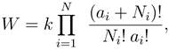
FD gases. The statistical entropies of both are expressed in the form
where
is the total number of particles. Also
Ni is the number of
indistinguishable particles in zone
i,
G is the total number of zones,
ai is an application specific measure of the number of cells in this zone, and
k is Boltzmann’s constant. The zoning criteria is the approximate energy level of particles in the cells. The fact that both of the
BE and
FD distributions arise from the same general form simplifies much of the subsequent analysis since specific results obtained for one apply automatically to the other as well.
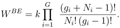
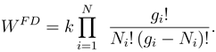
When
ai=
gi − 1,
gi being the number of cells in zone
i, (8) is identified as the
BE distribution function. That is
The generic term in this product, (
gi +
Ni − 1)!
/Ni!(
gi − 1)!, is the number of ways
Ni indistinguishable particles can be distributed among
gi cells.
The ecosystem ansatz is to distribute Ni organisms, or units of biomass, in zone i, which contains gi cells. The mass equivalent of the Ni organisms in zone i is mi. The Ni could come from Volterra type models as studied by Kerner (1957, 1959), allometric equations as reported by Brown et al. (2002), or, best of all, observations.
The final step in the construction of an ecosystem phase space is to specify a criterion for zoning the phase space. Quantum statistics uses particle energy as the zoning criterion. What is an ecosystem counterpart of particle energy? I propose metabolic energy, which here is defined as the product of metabolic rate and life span or regeneration time. Specifically this is
where
Ri and
τi are defined by (2) and the subscripts refer to the
ith zone.
The
FD problem in quantum statistics arises when only one particle can occupy a cell. This results from the Pauli exclusion principle that no two Ferminons, for example electrons, can be in the same state. This distribution function is recovered from (8) by setting
ai=
gi −
Ni:
Is species exclusion an ecosystem counterpart to (11)? Species exclusion has a long and contentious history in ecology. See Bastolla et al. (2005) for a succinct review. In essence, the underlying idea is that there is only one surviving species when two or more attempt to occupy the same ecological niche. In this case Ni is the number of species and gi is the number of ecological niches in zone i.
A major problem with any species exclusion theory is that there is no absolute specification of ecological niche. Perhaps the specification of phase space down to the microbial level will circumvent this
Table 1.
Comparison of characteristics of quantum and ecosystems.
Table 1.
Comparison of characteristics of quantum and ecosystems.
| Quantity | Quantum | Ecosystem |
|---|
| Number of Bosons in zone i | Number of organisms or amount of biomass in metabolic energy band i |
| Number of cells in zone i. | Number of cells occupied by biomass in metabolic energy band i |
| Number of Fermions in zone i | Number of species in metabolic energy band i |
| Number of cells in zone i | Number of ecological niches in metabolic energy band i |
objection, and so the
FD model may apply. This requires ecological niches to be defined in terms of microbial scales. Of course, this also requires an
hE for niches; a situation not unlike the different cell sizes for the quantum
BE and
FD problems.
A synopsis of the applications of the
BE and
FD models is given in
Table 1.
In the BE and FD quantum statistics problems the cell sizes are h3 and h3/2 respectively, i.e. both are simply proportional to the same uncertainty parameter. The ecosystem problem requires a more general approach since it not clear that the same hE applies to both problems. This issue is not addressed here, however.
The gi are useful for comparing similar ecosystems, or assessing the impact of habitat change in existing ecosystems. Specifically, a change of habitat changes the number of cells that can support a metabolic energy level. Then the gi will change and consequently WBE. Similarly a change in habitat will alter the number of niches available for species with similar metabolic energy levels. This change is quantified by a change in WFD.
Note that both the BE and FD models arise in quantum statistics because of the requirement that quanta are indistinguishable; i.e., there is no characteristic that can distinguish one quantum from another. This contrasts with the Boltzmann entropy function, widely used in ecology, in which individual organisms are distinguished. However, since the phase space proposed here is microbial based, it is appropriate to drop the requirement for distinguishability. Presumably there is no way to distinguish one specimen of Staphylococus from another.
3. Ecosystem equilibria
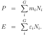
The entropy principles formalized in the previous section are completely general as they are applicable to any ecosystem at any time. Moreover, they can serve as a basis for a precise statement of equilibria for ecosystems. To arrive at this it is necessary to consider the total amount of biomass
P and metabolic energy
E of any ecosystem as
The
mi in the first of (12) are mass equivalents of the organisms in each metabolic energy zone. They convert the number of organisms
Ni in that zone to the biomass in that zone. Their use here means that with the
BE model the summation of the first of (12) gives the total biomass in the ecosystem. The
FD model deals with the number of species in zones so the
mi are representative of an individual’s mass for the appropriate species. The same comments apply to the total metabolic energy
E of an ecosystem. Note that the weighting
εi is by the metabolic energy in zone
i as specified by (10).
It is reasonable to assume that an ecosystem in equilibrium has reached the maximum diversity that the environment can sustain. A phase space entropy as defined by (9) or (11) seems appropriate for a measure of diversity. However, in studying equilibria it is more convenient to use the logarithm of these two equations, i. e.
Ecosystem equilibria requires that (12) be constant and (13) a maximum. Since all three are functions of
Ni, these conditions are satisfied if their variations with respect to
Ni are zero. Formally this is
Here
λ and
β are Lagrangian multipliers that arise in the variational problem from the requirement that (12) must be constant if equilibrium is to be achieved. They are determined by system macroproperties.
λ can be related to the total amount of biomass in the ecosystem, while
β can be determined from metabolic energy constraints. Below it is related to an environmental temperature through the first law of thermodynamics. Finally,
δ = ∑
i (
∂/
∂Ni)
δNi is the variational operator.
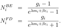
Equation (14) is satisfied by
When multiplied by
mi, the distributions given by (15) give the distribution of mass or species in the
ith metabolic energy zone when an ecosystem is in equilibrium with its environment. Multiplication by
εi gives the metobolic energy of that zone. Finally, if ecosystems are considered as a classic thermodynamic systems, then application of the first law of thermodynamics gives
where Θ is absolute temperature.
This result is quite similar to the allometric equations for species distributions that included metabolic rates e−εi/kΘ reported by Brown et al. (2004). It agrees exactly with their results when λ ≪ 1. It also reinforces the notion that a thermodynamic interpretation such as (16) applies to ecosystems. Equation (15) shows that in terms of biomass, low metabolic energy organisms or species dominate ecosystems. This is the ecosystem counterpart of the quantum statistics result that there are many more low energy than high energy particles in a quantum gas.
In quantum statistics, λ is determined by the conservation of mass. It is worth noting that for photons, mass is not conserved. In that case λ = 0. For λ ≪ 1 both distributions in (15) collapse to the Maxwell distribution Ni = gie−βεi, an approximation that holds for many quantum physics applications. This may turn out to be true in many ecological applications. However, further investigation is required before applying this simplification to ecosystems.
In contrast to their exponental dependence on inverse temperature, the BE and FD distributions are linearly proportional to the number of cells occupied by a particular metabolic energy band. These distributions are also of the form of allometric equations for species density such as those developed by Brown et al. (2004). The number of cells in a zone is a direct reflection of macro-ecosystem characteristics. A change of habitat will alter the number of cells available for certain individuals or species within certain metabolic energy bands.
4. Discussion
This paper gives a paradigm for a statistical description of ecosystems based on a discrete phase space. Phase space cell characteristics are determined by microbial scales. This is in analogy with quantum statistical mechanics where the fundamental phase space cell is determined by Heisenberg’s constant. Estimates of the ecosystem cell parameter hE are only about three orders magnitude larger than ħ. However, it is likely that the hE’s for the two ecosystem models will not be as simply related as they are for the BE and FD quantum models. The similarity in magnitude of the quantum and ecosystem uncertainty parameters is due to the long time scales for biological systems relative to those of quantum systems. The significance of an hE based on microbial scales is that it provides a formal link between the largest and smallest life forms in ecosystems. Moreover, this paradigm would apply to extraterrestrial ecosystems.
Several aspects of this approach should be noted. First, precise conditions for equilibrium are prescribed. These are obtained from the principles of conservation of biomass and energy, along with the principle that at equilibrium the entropy is a maximum for the prescribed biomass and energy. This gives formula for the distribution of biomass based on metabolic energy. Moreover, the entropies used here can be estimated from existing data using standard allometric equations, whether or not equilibria is established.
A second aspect is entropy as a measure of diversity. See Brooks and Wiley (1988) for a perspective and Bastolla et al. (2001, 2005) along with Kobayashi et al. (2005) for recent applications. Brooks and Wiley (1998) and coworkers in particular have made considerable progress on this topic using information theory concepts. Their analysis is based on a Boltzmann or Shannon entropy and relies on a theorem that a system whose entropy is greater than the sum of its constituent subsystems and is not concave can be in equilibrium even if the system entropy is not a maximum. See Landsberg and Tranah (1980) and Landsberg (1984a,b) for the theoretical development of this idea. They introduced the important concept of “capacity” to characterize the upper bound of ecosystem development. This is the maximum entropy that the system can achieve. Both Brooks and Wiley (1998) and Landsberg (1984b) suggest that in reality observed systems will always have entropies less than their capacities.
In view of this it is appropriate to ponder the capacity of
BE and
FD systems. To this end first consider the ultimate capacity of a Boltzmann system,
N !. This occurs when there is at most just one element in any cell. However, at equilibrum, as defined in
section 3, many cells will be empty. The entropy then is a maximum
for the prescribed biomass and total metabolic energy. This is less than the maximum entropy that could be achieved for a uniform distribution of mass over phase space. Thus, to achieve the maximum capacity requires disturbing the equilibrium by adding or redistributing biomass so that it is equally distributed among the cells in phase space. Essentially this is what happens when a pond stagnates. The pyramid distribution of metabolic organisms, typical of a healthy pond, is replaced by microbes and/or lilies and phase space is completely uniform.
The use of entropy in this context has consequences that are independent of the mathematical form of entropy used. The quantification of diversity in the guise of entropy should be based on both the environment and population or biomass. As habitat changes (thus altering the gi’s) then the entropy must change. Thus an equilibrium distribution of species or ecological niches with one set of gi’s must change as the latter change. In this sense diversity is more than just a measure of the number of species in an ecosystem. It is a measure of the number of ways an environment can support organisms in prescribed metabolic energy ranges. Present concern about the loss of diversity acknowledges that the phase space of the global ecosystem is changing to the disadvantage of many high metabolic energy organisms. A phase space based approach, such as used here, quantifies this idea.
The theoretical construction presented here seems well suited to analysis of “what if?” scenarios that arise with global change. Habitat changes can be quantified by changes in the gi’s. Similarly the impact of loss of species is quantified by changes in the Ni’s.
On the other hand, a phase based statistical approach in ecology has even greater limitations than quantum statistics does in physics. It cannot provide details of organism interactions, or replace Volterra or inertia models of ecosystems as used by Ginzburg (1998). Its principal role is to provide useful conceptual tools for synthesizing and characterizing macro properties.
Skeptics may ponder: “In quantum mechanics any particle can fit into any cell in phase space. So can an elephant fit into one hE determined by microbial scales?” Actually quantum mechanics cannot determine whether a particular particle is in a particular cell since the particles are indistinguishable. Instead quantum mechanics says how many particles are in particular zones. The essential point is that the biomass of all elephants fits into a zone composed of a small portion of the cells in phase space. This is the power of zoning by metabolic energy levels. The issue is to determine how many cells are occupied by organisms within specified metabolic energy bands.
As just noted quantum statistics says that the question of which particle is in what cell is unanswerable and thus irrelevant. In analogous fashion high resolution observations of ecosystems add little information about the macrostate of an ecosystem even though they provide important details on organism interactions. This is the gist of Brown’s (1995) meaning for macroecology. The same distinction is made between thermodynamics and statistical mechanics by physicists.
As just noted quantum statistics says that the question of which particle is in what cell is unanswerable and thus irrelevant. In analogous fashion high resolution observations of ecosystems add little information about the macrostate of an ecosystem even though they provide important details on organism interactions. This is the gist of Brown’s (1995) meaning for macroecology. The same distinction is made between thermodynamics and statistical mechanics by physicists.
The phase space prescription based on microbial scales is just one of an infinite number of possibilities. It may be appropriate to base phase space cell characteristics on other scales, or even abandon the constraint that it have the same dimensions as ħ. Nevertheless entropies based on a phase space approach can be the launching pad for studying fluctuations and non-equilibrium dynamics of ecosystems just as it is in quantum statistics. It would be interesting to apply these ideas to see if observed variability in populations reflect natural fluctuations around a robust equilibrium or whether they reflect evolution toward a new equilibrium. In addition it might be useful to examine ecosystems in extreme environments using a phase space paradigm.
The gist of this paper is that a phase space ansatz, generally patterned after the quantum statistics, has a role in ecology. As eloquently stated by Ginzburg and Colyvan (2004), quantum statistics is just a metaphor. Metaphors have played an important part in the long history of cross fertilization between scientific disciplines. This history also suggests that applications of these ideas for ecosystems will result in interesting and challenging deviations from the purely quantum statistics ansatz.