Review of Processing and Interpretation of Self-Potential Anomalies: Transfer of Methodologies Developed in Magnetic Prospecting

Abstract

The self-potential (SP) method is one of the most inexpensive and unsophisticated geophysical methods. However, its application is limited due to the absence of a reliable interpreting methodology for the complex geological-environmental conditions. To exclude disturbances appearing in the SP method, a few ways for their removal (elimination) before quantitative analysis are presented. A brief review of the available interpretation methods is included. For the magnetic method of geophysical prospecting, special quantitative procedures applicable under complex physical-geological environments (oblique polarization, uneven terrain relief and unknown level of the normal field), have been developed. The detected common peculiarities between the magnetic and SP fields make it possible to apply the advanced procedures developed in magnetic prospecting to the SP method. Besides the reliable determination of the depth of anomalous targets, these methodologies enable the calculation of the corrections for non-horizontal SP observations and to determine the orientation of the polarization vector. For the classification of SP anomalies, is proposed to use a new parameter: the ‘self-potential moment’. The quantitative procedures (improved modifications of characteristic point, tangent techniques and the areal method) including the determination of the SP vector and SP moment, have been successfully tested on models and employed in real situations in mining, archaeological, environmental and technogenic geophysics. The obtained results indicate the effectiveness of the presented methodologies.

1. Introduction

The Self-Potential (SP) method is based on the study of natural electric fields (in some cases, this method is named as ‘spontaneous polarization’). The term “natural” here means that the field is not created by an external artificial source. Permanent electric fields arise in the course of redox, filtration, and diffusion-adsorption processes in the upper part of the geological section. The registration of these fields is the goal of the SP method, and the geophysical interpretation of the parameters generating this field is the main purpose of SP data examination. An oxidizing object (e.g., ore body, archaeological or environmental target) is a galvanic cell, the existence of which requires: (1) the contact of electric conductors with different types of conductivity (electronic and ionic), and (2) the difference in the redox conditions at different contact points of these conductors. An appearance of these conditions is usually impossible without underground water contact [1].

In the geological section, the conditions for the formation of a galvanic cell arise on the targets with electronic conductivity, if these bodies are in the water-saturated rocks with ionic conductivity. The change in the redox conditions at the contact point of the electronic conductor (anomalous target) and the surrounding medium is associated with a decrease in the oxygen content with a depth.

Fox’s [2] SP observations at copper vein deposits in Cornwall (England) laid the foundation of the application of all electric methods in geophysics as a whole. SP is an effective, prompt and comparatively simple geophysical method. Equipment for SP method is one of the most inexpensive in the field of geophysics (

Table 1. Average prices for geophysical potential field equipment (on the basis of author’s personal contacts with the various manufacturers of geophysical equipment (January 2021)).

Method	Gravity	Magnetic	Resistivity	Self-Potential
Price of equipment US $	60,000–110,000	20,000–25,000	35,000–55,000	150–200

).

Conventional equipment employed in the SP method consists of a microvoltmeter, a pair of non-polarizable electrodes, cable and CuSO₄ solution (the latter is necessary for the better contact of employed electrodes with the environment).

Usually (not always, depending on geological and environmental peculiarities of studied deposit (cite)), ground penetration radar (GPR) and electric resistivity tomography (ERT) produce more detailed geophysical-geological information. However, they are much more expensive and, most importantly, water content in subsurface strongly complicates application of these methods. At the same time, the presence of water for the SP method is only positive factor, since it enables to increase SP anomaly intensity, e.g., [3,4].

The SP method is employed in mining geophysics e.g., [3,5,6,7,8,9,10,11,12,13,14], archaeological geophysics e.g., [15,16,17,18,19,20,21,22,23], environmental geophysics e.g., [24,25,26,27,28,29,30,31] and technogenic geophysics [32,33,34,35]. Application of quantitative analysis in the SP method for solving other geological-geophysical problems is beyond the scope of this study.

The values of SP anomalies vary in wide range: from fractions of a millivolt in detailed studies to several Volts in regional surveys (the origin of the latter has not been determined until recent time) [3,8,12,13,15,23,26,30,32,34].

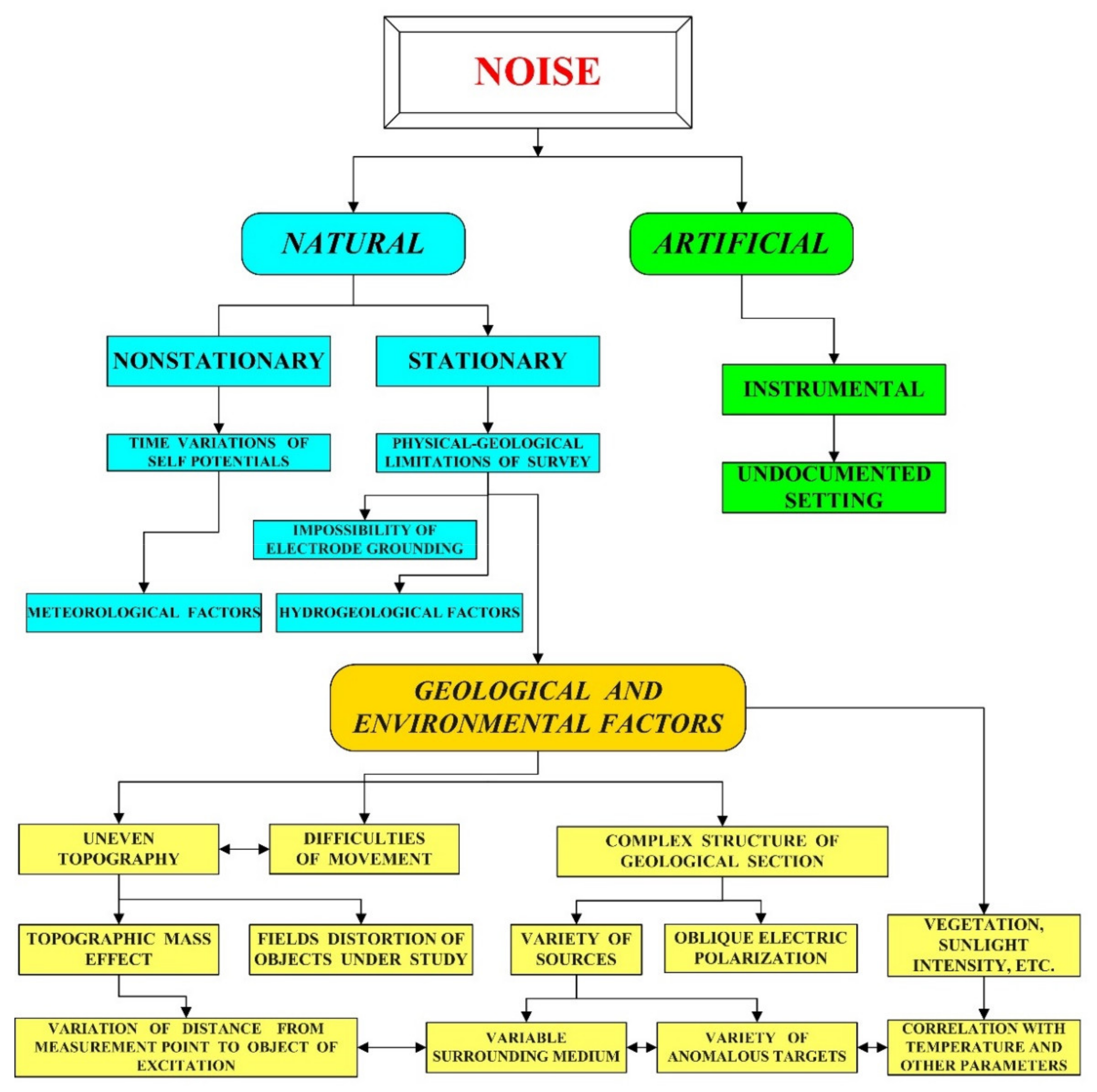
2. Self-Potential Observations: Analysis of Disturbances

The main kinds of noise appearing in the SP method are compiled in a block-scheme (Figure 1). Some of these noise effects are considered below in detail.

2.1. Electrode Noise in SP Method

Although the fact that SP electrode is called as “non-polarizable”, after some time it accomplishes some polarization effects from the surrounding media. However, taking into account that we measure the value ∆U (U₁ − U₂), it is important to keep not an absolute non-polarizability, but an equivalent polarization on both of the applied electrodes. For checking this equivalent, the following procedure can be employed in field conditions (of course, measurements in a physical laboratory are more precise). We can write a trivial equation for the first electrode: U₁ + e₁ (U₁ is the first “medium” signal, and e₁ is the noise accumulated in the first electrode). For the second electrode, correspondingly, we have U₂ + e₂ (U₂ is the second “medium” signal, and e₂ is the noise of accumulated in the second electrode). According to [3], we measure:

$$\mathrm{\Delta }{U}_1=\left(U_1+e_1\right)-\left(U_2+e_2\right)$$

(1)

where ∆U₁ is the self-potential field generated between the first and second SP electrodes.

Let us change electrodes by their places. In this case, we will obtain:

$$\mathsf{\Delta }{U}_2=\left(U_1+e_2\right)-\left(U_2+e_1\right)$$

(2)

where ∆U₂ is the self-potential field generated between the second and first SP electrodes.

After this, calculating a difference between ∆U₁ and ∆U₂, we receive:

$$\mathrm{\Delta }{U}_1-\mathrm{\Delta }{U}_2=\left[U_1+e_1-U_2-e_2\right]-\left[U_1+e_2-U_2-e_1\right]=2\left(e_1-e_2\right)$$

(3)

or

$$\left(e_1-e_2\right)=\frac{\mathrm{\Delta }{U}_1-\mathrm{\Delta }{U}_2}{2}$$

(4)

If the value $\left(e_1-e_2\right)$ is significant (e.g., ≥3 mV), the noised electrodes must be replaced by new ones. A similar methodology for the electrode noise detection was suggested in [36].

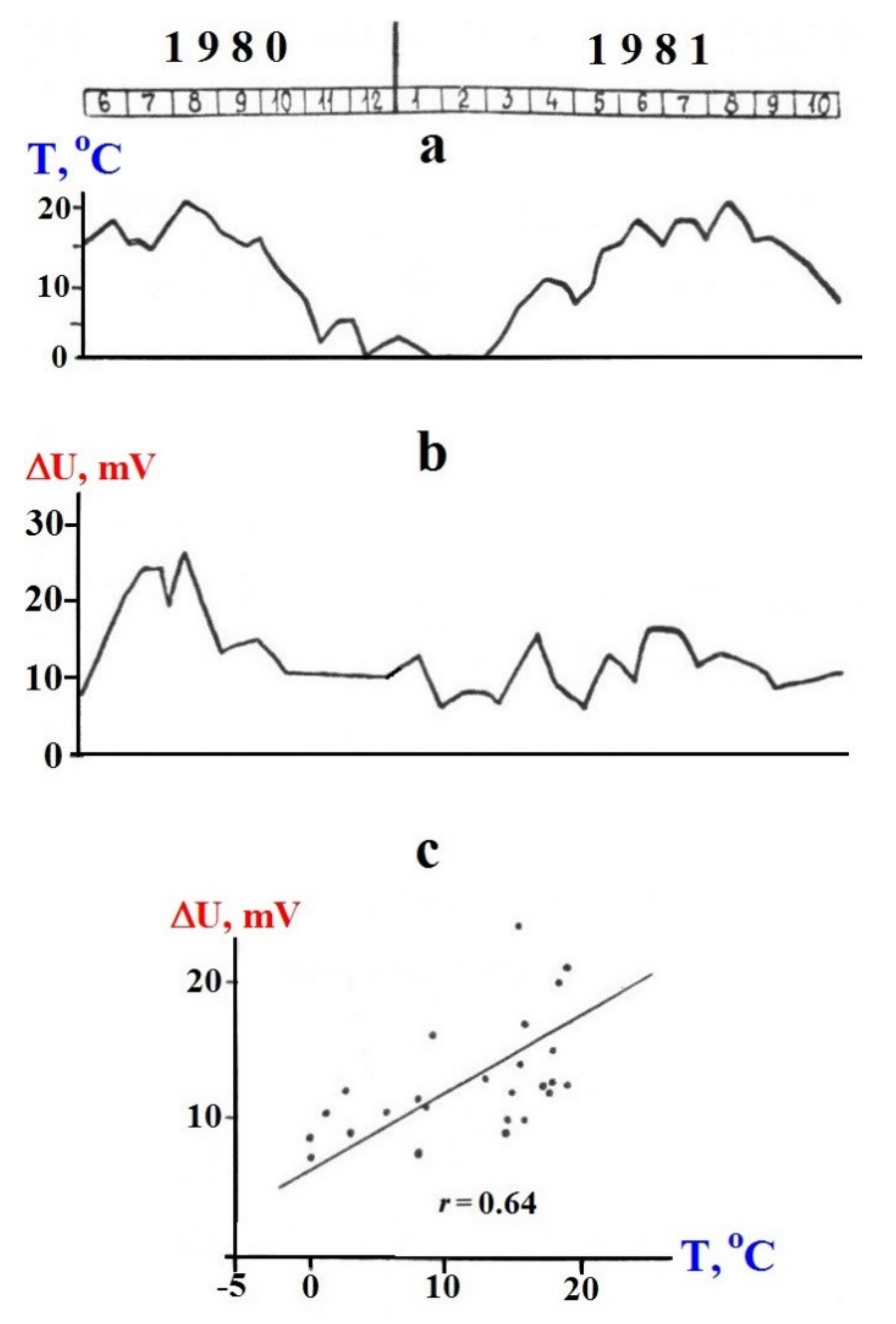
2.2. Temporal Variations in SP Method

Parasnis [4] carried out SP measurements of the same profiles in the Akulla region (Sweden) seven times during the period of 1960–1967. These measurements indicate a good repeatability despite the fact they were conducted under different climatic conditions. Similar investigations performed by other researchers, e.g., [3,37], basically confirm the good repeatability of the different SP time observations.

For the estimation of accuracy ε of SP field measurements, the following trivial formula is often employed in various geophysical methods:

$$\epsilon =\pm {\left(\frac{{{\displaystyle \sum }}_{i=1}^N{\delta }^2}{N}\right)}^{1/2}$$

(5)

where N is the total number of SP observations, and δ = (∆U_init − ∆U_repeat), where ∆U_init means the ordinary (initial) measurements, and ∆U_repeat—the repeated measurements. The number of repeated measurements should be at least 8–10% of the total number of observations. If the value of ε exceeds some a priori assumed value (this value usually depend on the concrete spread of the SP amplitudes), results of SP survey can be rejected as non-reliable.

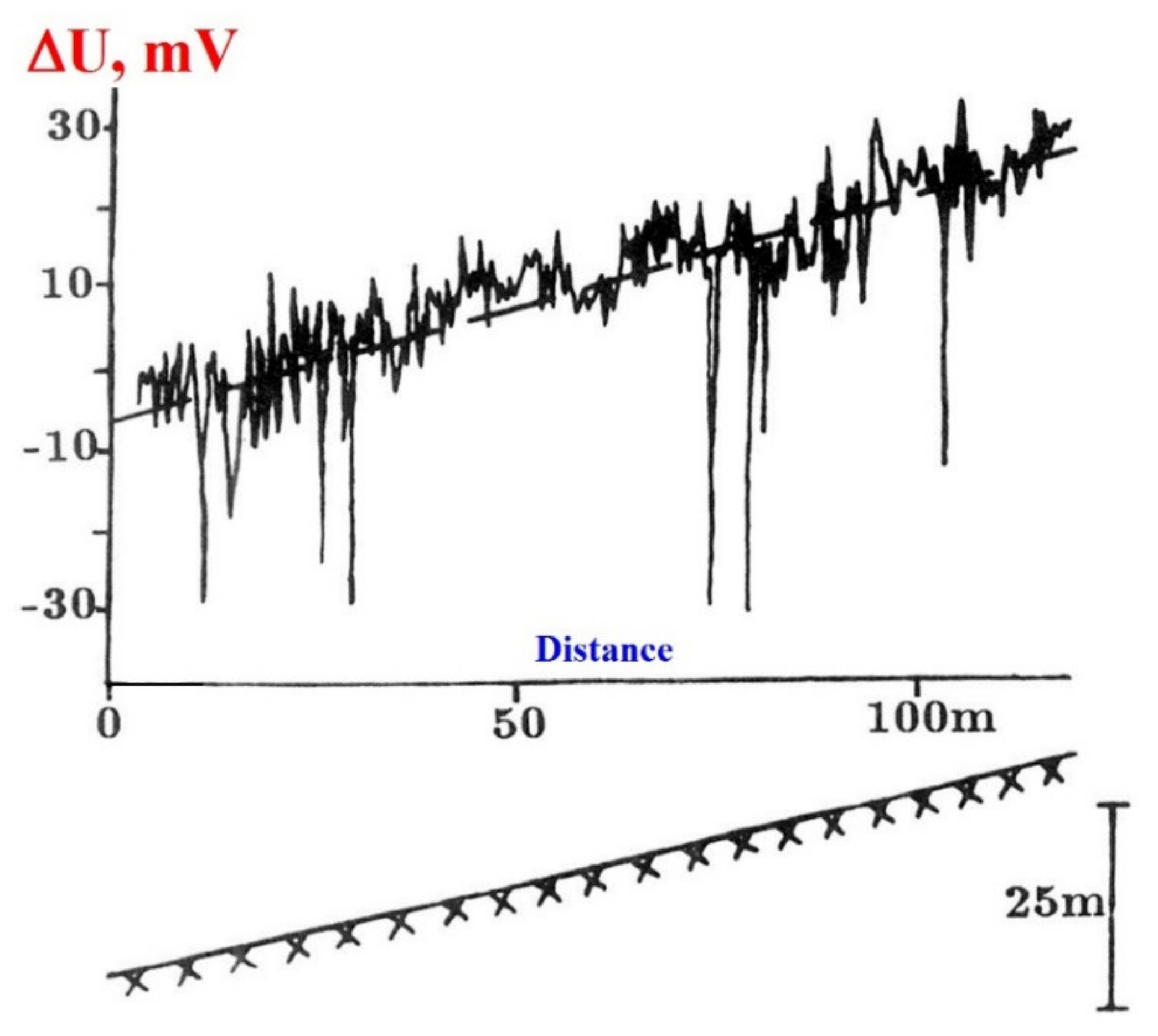
2.3. Terrain Relief Correction

In the SP method, terrain relief influence is two-fold. On the one hand, negative SP anomalies caused by electromotive force can be created over the positive topographic forms (this phenomena strongly depends on the peculiarities of underground water circulations). Comparison of the SP graphs with topographic data usually allows for the identification of anomalies of this type by the character mirror image of the terrain relief in SP anomalies [38].

From other side, as follows from the very detailed SP measurements of Ernstson and Schrerer [39], at the inclined topographic surface, the SP field increases directly with increases in the relief highs (Figure 2).

In the last case, for the elimination of the terrain relief influence, a correlation method developed in magnetic prospecting [38], and VLF studies [40] can be applied. The essence of this method is as follows. The method employs, for the removal of the terrain relief effect from the observed field, ∆U_obser, a linear least-squares relation ∆U_appr (application of more complex approximations (e.g., parabolic, etc.) is also possible):

$$\mathrm{\Delta }{U}_{appr}=c+bh$$

(6)

where h is the height of relief, b is the angle coefficient, and c is the free member.

Value ∆U_appr approximates the observed field as a function of elevation h (anomalous zones usually do not include the correlation field), and then we obtain the corrected (residual) field ∆U_corr, where the relief influence is essentially eliminated:

$$\mathrm{\Delta }{U}_{corr}=\mathrm{\Delta }{U}_{obser}-\mathrm{\Delta }{U}_{appr}$$

(7)

It should be noted that this correction only eliminates the effect of the inclined topographic masses with certain electric properties. Special methods allow for the calculation of the difference in altitudes of SP observations to the anomalous target on an inclined profile, which are considered later in this paper.

Wang and Geng [41] studied the problem of terrain correction in the SP method in detail in several field examples. They noted that the mechanism of SP anomalies formed by terrains is rather complex, and therefore it is difficult to obtain the corresponding analytical formulas. Three types of relief fitting were applied: (1) linear, (2) quadratic and (3) exponential. After careful analysis, it was concluded that the linear fitting is more optimal since it does not create factious anomalies [41]. Thus, this investigation confirms the application of the aforementioned linear least-squares correlation method.

2.4. Calculation of SP Anomaly Distortion Due to Observations on Uneven Surface

SP anomalies (and anomalies of other potential fields) distort due to observations on uneven surfaces (and correspondingly, from different distances to anomalous objects). This disturbing effect usually is calculated at the end of the interpretation process (see Section 4.1).

2.5. Net Justification in Areal Observations

Net justification of SP data is conventionally performed by the use of procedure identical to justify the observations in gravity and magnetic prospecting, e.g., [42]. Other strategies for removing this effect are presented in [43].

2.6. Influence of Meteorological Factors

Many scientists note that rain increases the intensity of SP anomalies, e.g., [3,4,43]. Therefore, occasionally, an artificial irrigation of site intended for SP research is recommended.

2.7. Presence of Magmatic Associations

Obviously, the development of magmatic associations (or other kinds of hard geological rocks) in a site destined for field investigations does not allow for the grounding of SP electrodes. In such cases, it is impossible to carry out the SP measurements. The same reason may limit the water circulation at the subsurface, which can weaken, or even completely cancel a generation of the SP anomalies.

2.8. Some Environmental Factors

The SP anomaly level may affect some environmental factors. One of these factors is the shadowing of a part of the investigated area. For instance, Revil and Jardani [43] documented the fact that the difference between the SP electrodes placed in cold and warm media may exceed 10 mV. Another factor is a presence of some hygrophilous plants (e.g., hazel and almonds) whose roots can pick over a lot of moisture from the upper part of the geological section (thereby hindering the SP anomaly generation).

Ernstson and Schrerer [39] monitored SP and temperature anomalies during 15 months in 1980–1981 (Figure 3). The correlation between SP and soil temperature is interpreted as result of the influence of the thermal diffusivity and convection processes in the subsurface [39]. Between these parameters, a correlation of r = 0.64 was established. It is a low relationship, but in any case, should be taken into account.

Perrier and Morat [44] also detected a correlation between the amplitudes of the SP variations and soil temperatures. According to these authors, the state of the soil in the first 30 cm seems to play an important role. The authors concluded that the joint monitoring of electric potential and temperature appears to be a powerful tool to monitor the underlying soil processes [44].

An essential relationship between the SP data and temperature values recorded in boreholes at intermediate and large depths was established for the Cerro Prieto geothermal field (Baja California, NM, USA) [45]. An existence of this phenomenon under normal thermophysical conditions is not studied yet in detail.

3. Review of Available Quantitative Interpretation Methods

The calculation of theoretical anomalies due to SP has long been based primarily on Petrovsky’s [46] solution, which was derived for a vertically polarized sphere [37]. Later on, some substantial solutions for sheet-like bodies and inclined plates were obtained [3]. The electric polarization vector was generally considered to be directed along the sheet-like body dipping (along the longer axis of the conductive body).

Other methods of SP anomaly quantitative interpretation includes anomalous body with a simple geometrical shape which approximates the anomaly source. Its parameters (i.e., the depth, the angle between the horizon and the direction of the polarization vector) are usually determined by: (1) graphically using characteristic points of the anomaly plot, or (2) by trial-and-error method consisting of visual comparison of the observed anomaly with a set of master curves [3].

Zaborovsky [37], Semenov [3], and Murty and Haricharan [47] applied the SP anomaly generated by plates to the following formula:

$$U\left(x\right)=\frac{j\rho }{2\pi }\ln \frac{r_1^2}{r_2^2}$$

(8)

where j is the current per unit length, ρ is the host medium resistivity, r₁ and r₂ are the distances from the plate left and right ends to the observation point.

Fitterman [48] gave the method of SP anomaly calculation for field sources of an arbitrary shape based on numerical integration using Green’s function. This potentially promising approach is highly computer intensive and does not provide sufficient accuracy.

A few groups of authors performed spatial-frequency analysis of SP anomalies produced by polarized bodies of various geometrical shapes [49,50,51,52,53]. For instance, Rao et al. [49] analyzed the Fourier amplitude and phase spectra of SP anomalies to evaluate the parameters of the sheet; the application of this method on two anomalies (synthetic and field data) has given satisfactory results. 1D and 2D spatial frequency analysis of SP anomalies from the polarized sphere initiated in [52] was successfully evaluated in [53].

A series of publications [54,55,56,57,58] provided a large number of methodological approaches. However, these approaches (based mainly on application of the gradient analysis and calculation of derivatives) by their common usefulness, have not caused a quantitative jump in this field.

Gibert and Pessel [59] applied the continuous wavelet transform for the localization of SP anomalies. The wavelet analysis provided both an estimate of the location and of the nature of the target responsible for a given self-potential signal. The wavelet-based techniques as well as analytic signals were employed to interpret SP anomalies caused by subsurface fluid flow in Mt. Etna [60].

Patella [61] suggested an application a tomographic presentation of SP images. It consisted of scanning the geological-geophysical section through SP profiles, by the unit strength elementary charge, which is given a regular grid of coordinates within the section. At the each point of the section the charge occurrence probability function is calculated. The complete set of calculated grid values is employed to draw colored sections. This method was evaluated in [62].

Mendonça [63] employed the Green functions to simplify the evaluation of SP anomalies from buried conductors. This approach was used by this author to simulate geoelectric targets in mineral exploration and to obtain current source terms by inverting the SP data set.

Srivastava and Agarwal [64] developed the Enhanced Local Wave number technique wherein the nature of the causative source has been determined by computing structural indices based on its horizontal location and depth. This approach was tested on several mineral deposits with complex ore body distribution (among others, in the Rajasthan Copper belt (India) and sulphide deposit in Quebec (Canada)).

There are a number of recent interpretation techniques based on minimizing the difference between the observed and theoretical anomalies. The minimization is achieved by sequential optimization of the interpretation parameters through computer-aided iterations e.g., [65,66,67,68]. These techniques are usually effective under simplified physical-geological conditions.

An attempt to apply the neural network approach to compute the shape factor and depth of the causative target from SP anomaly was undertaken in [65]. The validity of the neural network inversion is demonstrated through the SP data taken from a graphite body in the southern Bavarian Woods (Germany). A comparable and acceptable agreement is shown between the results of inversion derived by the neural network and those from the real field data. Without denying the general promise of this approach, it should be noted that some inconclusiveness of examples given in this work.

Hristenko and Stepanov [66] demonstrated a system of 2D modeling of an SP field from several anomalous bodies with introduced Gaussian noise under conditions of uneven relief. Some applied transformations allowed for the exclusion of the effect of near-surface geological inhomogeneities from the total SP field and to enhance anomalies from the buried targets.

Gobashy et al. [67] proposed a method based on utilizing the optimization algorithm, which is an effective heuristic solution to the inverse problem of SP field due to a 2D inclined bed. The realization of this perspective algorithm under complex physical-geological conditions should be continued. Rao et al. [68] proposed a global optimization methodology expressed in the development of inversion algorithm for 2D inclined plates. Absence of the geological sections in the mentioned work complicates the examination of this methodology.

The procedure based on the interpretation of potential anomalies due to simple geometrical structures using Fair function minimization [69] is of certain interest. Giannakis et al. [70] suggested a hybrid optimization scheme for SP measurements due to multiple sheet-like bodies. This procedure demands a wide verification on concrete field examples. Of special interest is the recent research of [31], who developed the least-square subspace preconditioned method to compute the known Tikhonov solution to reliably detect the depth and the shape of shallow electrical current density sources.

Fedi and Abbas [11] proposed the ‘depth from extreme points method’ and employed it on several models and field examples. The method yields estimates of the source horizontal location, depth (top or center), and geometry.

Kilty [71] published a paper that acknowledged the analogy between the current density of SP and magnetic induction. This author suggested interpreting SP anomalies based on the conventional methods developed for magnetic prospecting. However, the proposed methodologies are not effective for complex physical-geological conditions. A similar approach, but with the improved interpretation methodology (specially developed for conditions of the rugged terrain relief, oblique polarization and unknown level of the normal field) was proposed in [38]. Eppelbaum and Khesin [72] proposed a new elaboration of the interpretation process. The present paper shows a final generalization of this approach.

4. Some Common Aspects of Magnetic and SP Fields

The magnetic field is a potential one (when value of target’s magnetization is not very high) and satisfies Poisson’s equation:

U_a = −grad V

(9)

where U_a is the anomalous magnetic field and V represents the magnetic potential.

SP polarization is generated by the spontaneous manifestation of electric double layers on contacts of various geological (or environmental and artificial) objects. The electric fields E of the electric double layer l caused by natural electric polarization are defined as the gradient of a scalar potential П_i:

$$E_{\mathrm{SP}}=-\mathrm{grad}{\mathrm{\Pi }}_i$$

(10)

The potential ${\mathrm{\Pi }}_i$ satisfies Laplace’s equation everywhere outside of the layer l [73].

Jardani et al. [74], in addition to Equation (10), proposed the following expression for explanation of SP pattern generating by geothermal flow:

$$\mathrm{grad}\cdot \left(\sigma \mathrm{grad}\mathrm{\Pi }\right)=\mathrm{grad}\cdot J_s=\zeta$$

(11)

where σ is the conductivity (in S/m), J_s is the current density vector (in A/m²), and ζ is the volumetric current density (in A/m³). Equation (11) also indicates a potential character of the SP field.

Analytical expressions for some of the interpreting models for magnetic and SP fields are presented in

Table 2. Magnetic and SP fields: Comparison of analytical expressions for some interpreting models.

Field	Analytical Expression
Magnetic	Thin bed (TB)           (12)	Point source (rod)    (13)
	$Z_v=2J2b\frac{z}{x^2+z^2}$	$Z_v=\frac{mz}{{\left(x^2+z^2\right)}^{\raisebox{1ex}{$3$}\!\left/ \!\raisebox{-1ex}{$2$}\right.}}$
Self- Potential	Horizontal circular cylinder (HCC)  (14)	Sphere        (15)
	$\mathrm{\Delta }U=2\frac{{\rho }_1}{{\rho }_1+{\rho }_2}{U}_0{r}_0\frac{z}{x^2+z^2}$	$\mathrm{\Delta }U=\frac{2{\rho }_1}{2{\rho }_2+{\rho }_1}{U}_0{R}^2\frac{z}{{\left(x^2+z^2\right)}^{3/2}}$

(after [38]).

Here, Z_v is the vertical magnetic field component at vertical magnetization; J is the magnetization; b is the horizontal semi-thickness of TB; m is the magnetic mass (point pole magnetic charge); ${\rho }_1$ is the host medium resistivity; ρ₂ is the anomalous object (HCC or sphere) resistivity; $U_0$ is the potential jump at the source body/host medium interface; $r_0$ is the polarized cylinder radius; R is the sphere radius; x is the current coordinate; z is the depth of the upper edge of TB (center of HCC or sphere) occurrence.

Formulas describing the potential character of magnetic (Equation (9)) and SP (Equation (10)) fields are identical. The proportionality of analytical expressions (12)–(15) for magnetic and SP fields is obvious. It allows us to employ advanced interpretation methods developed in magnetic prospecting for conditions of rugged terrain relief in SP data analysis, the superposition of anomalies of different orders and oblique polarization (we assume that the SP polarization vector is analogue of the magnetization vector). It is supposed that the majority of interpretation methodologies developed for the magnetic and gravity fields are applicable for the SP method.

In several works, the application of some advanced procedures from the most developed potential fields (gravity and magnetics) was demonstrated using self-potential data. Akgün [75] applied the Hilbert transform (usually employed in gravity and magnetic prospecting) for analysis of SP data. Sindirgi et al. [76] successfully tested the SP anomalies method of the total normalized gradient developed in gravity prospecting. This investigation was continued in [77] with the application of the Euler deconvolution. Extended Euler deconvolution techniques were successfully tested in some mineral deposits and observations in deep boreholes [78]. Biswas [79] suggested the study of SP anomalies using the 2D analytic signal developed in magnetic prospecting.

Of special interest is the recently published research [80] where the author proposed the employment of the posterior distribution model of the SP anomaly inversion. The advantages of this approach are that the SP data may contain single and multiples of SP sources and this method does not require prior assumptions over the shape of the anomaly source.

4.1. Quantitative Analysis of SP Anomalies by the Use of Advanced Methodologies Developed in Magnetic Prospecting

The improved methods for SP anomaly analysis include characteristic points, tangents and areal methods (these methods are described in detail in the publications suggested to magnetic anomaly interpretation: e.g., [38,40,72,81,82]. Formulas for interpreting SP anomalies by use of the characteristic point method are presented in

Table 3. Formulas for quantitative interpretation of magnetic anomalies from bodies approximated by thin bed (TB) and horizontal circular cylinder (HCC) using the improved characteristic point method (after [40], with modifications).

Parameters Necessary for Examination	Parameters Derived from Anomalies from Models		Formulas for Calculation of Parameters Necessary for Quantitative Analysis
	Thin Bed	HCC	Thin Bed	HCC
Generalized Angle θ	d1, d2           d1r d1, d5          d1r, d5 $\begin{array}{l}{d}_1=x_{\min }-x_{\max }\\ d_2={\left(x_{0.5\mathrm{\Delta }{U}_A}\right)}_r-{\left(x_{0.5\mathrm{\Delta }{U}_A}\right)}_l\\ d_5=x_r-x_l\\ \mathrm{\Delta }{U}_A=\mathrm{\Delta }{U}_{\max }-\mathrm{\Delta }{U}_{\min }\end{array}$		$\tan \left(\theta \right)=d_2/d_1$ $\sin \left(\theta /3\right)=d_5/\sqrt{3}{d}_1$	$\cot \left(\theta /3\right)=\sqrt{3}\frac{\left(d_{1l}+d_{1r}\right)}{\left(d_{1l}-d_{1r}\right)}$ $\frac{d_5}{d_{1r}}=\frac{\sqrt{2}\cos \left(\theta /2\right)-1}{\sqrt{3}\cos \left({60}^{\mathrm{o}}+\theta /3\right)}$
Depth h0, hc	d1, d2, θ        d1r, θ d5, θ		$\begin{array}{l}{h}_0=\raisebox{1ex}{$\sqrt{d_1{d}_2}$}\!\left/ \!\raisebox{-1ex}{$k_{1,2}$}\right.,\hspace{1em}\hspace{1em}\hspace{1em}\hspace{1em}\hspace{1em}{h}_c=\raisebox{1ex}{$d_{1r}$}\!\left/ \!\raisebox{-1ex}{$k_{1r}$}\right.,\mathrm{where}{k}_{1r}\\ \mathrm{where}{k}_{1,2}\hspace{1em}\hspace{1em}\hspace{1em}\hspace{1em}\hspace{1em}\hspace{1em}\hspace{1em}=2\sqrt{3}\frac{\cos \left({60}^{\mathrm{o}}+\theta /3\right)}{\cos \theta }\\ =\frac{2}{\sqrt{\sin \theta \cos \theta }}\hspace{1em}\hspace{1em}\hspace{1em}\hspace{1em}\hspace{1em}\hspace{1em}\hspace{1em}{h}_c=\frac{d_{1r}}{d_{1r}-d_{1r}\left(\mathrm{\Delta }h\right)}\mathrm{\Delta }h\end{array}$ $h=d_5/k_5,\mathrm{where}$ $k_5=2\sqrt{3}\frac{\sin \left(\theta /3\right)}{\sin \theta }\hspace{1em}\hspace{1em}\hspace{1em}\hspace{1em}\hspace{1em}{k}_5=2\sqrt{2}\frac{\cos \left(\theta /2\right)-1}{\cos \theta }$
Horizontal Displacement x0, xc	h, θ, xmax, xmin,r $\begin{array}{l}{\left(x_{0.5\mathrm{\Delta }{U}_A}\right)}_r,\\ {\left(x_{0.5\mathrm{\Delta }{U}_A}\right)}_l\end{array}$		$\begin{array}{l}{x}_0=0.5(x_{\max }+x_{\min }{}_{,r})-h\cot \theta \end{array}$$x_0=h\tan \left(\frac{\theta }{2}\right)$	$\begin{array}{l}{x}_c=0.5\left(x_{\max }+x_{\min ,r}\right)-\\ h_c\frac{\sin \left({60}^{\mathrm{o}}+\theta /3\right)}{\cos \theta }+h_c\tan \theta \end{array}$$\begin{array}{l}{x}_c=0.5\left(x_r+x_l\right)+h_c\tan \theta -\\ \sqrt{2}{h}_c\frac{\sin \left(\theta /2\right)}{\cos \theta }\end{array}$
Normal Background $\mathrm{\Delta }{U}_{\mathrm{backgr}}$	∆Umin, ∆UA, θ		$\mathrm{\Delta }{U}_{\mathrm{backr}}=\mathrm{\Delta }{U}_{\min }+\mathrm{\Delta }{U}_A\frac{k_0}{1+k_0},\mathrm{where}$ $k_0=\frac{1-\cos \theta }{1+\cos \theta },\hspace{1em}\hspace{1em}\hspace{1em}\hspace{1em}\hspace{1em}{k}_0=\frac{{\cos }^3\left({60}^{\mathrm{o}}+\theta /3\right)}{{\cos }^3\left(\theta /3\right)}$
Self-Potential Moment	∆Ua, h0, hc, Q		$M_{\mathrm{\Delta }U}=\frac{1}{2}\mathrm{\Delta }{U}_a{h}_0$	$M_{\mathrm{\Delta }U}=\frac{\mathrm{\Delta }{U}_a{h}_c^2}{\left(3\sqrt{3}/2\right)\cos \left({30}^{\mathrm{o}}-\theta /3\right)}$

Indices “0” and “c” designate the thin bed (TB) and horizontal circular cylinder (HCC) models, respectively. Values h₀ and h_c are the depths to upper edge of TB and center of the HCC, respectively. Parameter ∆h designates measurements of self-potential field at different depths of the electrodes’ grounding.

. Several figures below display some peculiarities of the characteristic point and tangent methods application.

Preliminary results for SP anomalies to estimating HCC radius and length of horizontal upper edge may be obtained from 3D magnetic field modeling (taking into account a common similarity of these fields) (

Table 4. Nomenclature of variables applied for quantitative analysis of SP anomalies due to of thin bed and horizontal circular cylinder models (see Table 3).

Variable	Description
θ	Generalized angle reflecting the degree of SP anomaly asymmetry as a function relation of an anomalous body depth of occurrence, geometric form, value of polarization
x0	Horizontal displacement of projection of the middle of the upper edge of thin bed to the earth’s surface due to oblique polarization
xc	Horizontal displacement of projection of the center of the HCC to the earth’s surface due to oblique polarization
h0	Depth to the upper edge of thin bed
hc	Depth to the center of HCC
∆Umax	Maximum value of SP anomaly
∆Umin	Minimum value of SP anomaly
∆UA	Total amplitude of SP anomaly
d1	Difference of extremum abscissae for thin bed
d1r	Difference of extremum abscissae for HCC
d2	Difference of semiamplitude point abscissae
d5	Difference of inflection point abscissae
xr	Right inflection abscissae point
xl	Left inflection abscissae point
∆Ubackr	Normal background level of SP anomaly
$M_{\mathrm{\Delta }U}$	Self-potential moment for the models of thin bed or HCC

).

The improved versions of tangent and areal methods are presented in detail in [40,81,82].

4.2. SP Observations on an Inclined Profile

When potential geophysical anomalies are observed on an inclined profile, the obtained parameters characterize some fictitious body [13]. The transition from the parameters of fictitious target to those of real target is realized using the following expressions:

$$\left\{\begin{array}{l}{h}_r=h_f+x_{0f}\tan {\omega }_0\\ x_r=-h_f\tan {\omega }_0+x_{0f}\end{array}\right\}$$

(16)

where h is the depth of the body upper edge occurrence (or HCC (sphere) center), x₀ is the shifting of the anomaly maximum from the projection of the center of the anomalous body to the earth’s surface (produced by an oblique polarization), and ω₀ is the angle of the terrain relief inclination (ω₀ > 0 when the inclination is toward the positive direction of the x-axis), the subscripts “r” and “f” stand for parameters of real and fictitious bodies, respectively.

The direction of the electric self-polarization vector φ_p is calculated from the expression:

$${\phi }_p=90°-\theta$$

(17)

and on an inclined relief:

$${\phi }_p{,}_r=90°-\theta +{\omega }_0$$

(18)

The performed calculation of the vector φ_p direction on concrete field examples indicates that for the interpreting models closed to the model of a thin bed, the direction of this vector approximately coincides with the anomalous body-dipping. It enables us to obtain a supplementary interpretation parameter.

Besides the geometric parameters of the anomalous target, the self-potential moment can also be determined (see Table 3). For the models of thin bed and HCC, the self-potential moment can be calculated by the use of Equations (19a) and (19b), respectively (see also Table 3 and Table 4).

$$M_{\mathrm{\Delta }U}=\frac{1}{2}\mathrm{\Delta }{U}_a{h}_0$$

(19a)

$$M_{\mathrm{\Delta }U}=\frac{\mathrm{\Delta }{U}_a{h}_c^2}{\left(3\sqrt{3}/2\right)\cos \left({30}^{\mathrm{o}}-\theta /3\right)}$$

(19b)

where ∆U_a is the amplitude of SP anomaly (in mV), h₀ is the depth of the upper edge of thin bed (in meters), $h_c^2$ is the squared depth to the center of the HCC (in m²), and θ is the some generalized angle (see Table 3 and Table 4). The self-potential moment, by analogy with the magnetic field analysis, can be used for classification of various SP anomalies (and, correspondingly, hidden targets). Comparison of these values between themselves (separately for interpreting models of thin bed and HCC) indicates size of anomalous bodies, their depth and space position as well as ratio of electrochemical properties of the ‘anomalous target/surrounding medium’.

Initial methodologies for quantitative analysis of magnetic anomalies under complex physical-geological conditions for the model of the thick bed were presented in [38] and its significant evaluation (including the intermediate models between the thick and thin beds) was presented in [82].

For observation on an inclined profile, the real self-potential moment can be calculated as follows:

M_ΔU,r = M_ΔU,f cosω₀

(20)

Here, the subscripts “r” and “f” stand for a parameter of real and fictitious self-potential moments, respectively.

Undoubtedly, the calculation of all aforementioned parameters from SP data should be connected to a unified computerized system with the slight participation of an interpreter.

For the testing of some SP anomalies, the developed software for the 3D computation of the magnetic field (e.g., GSFC [13]) was applied. In this case, magnetic vector orientation can be utilized as analogue of the self-potential vector.

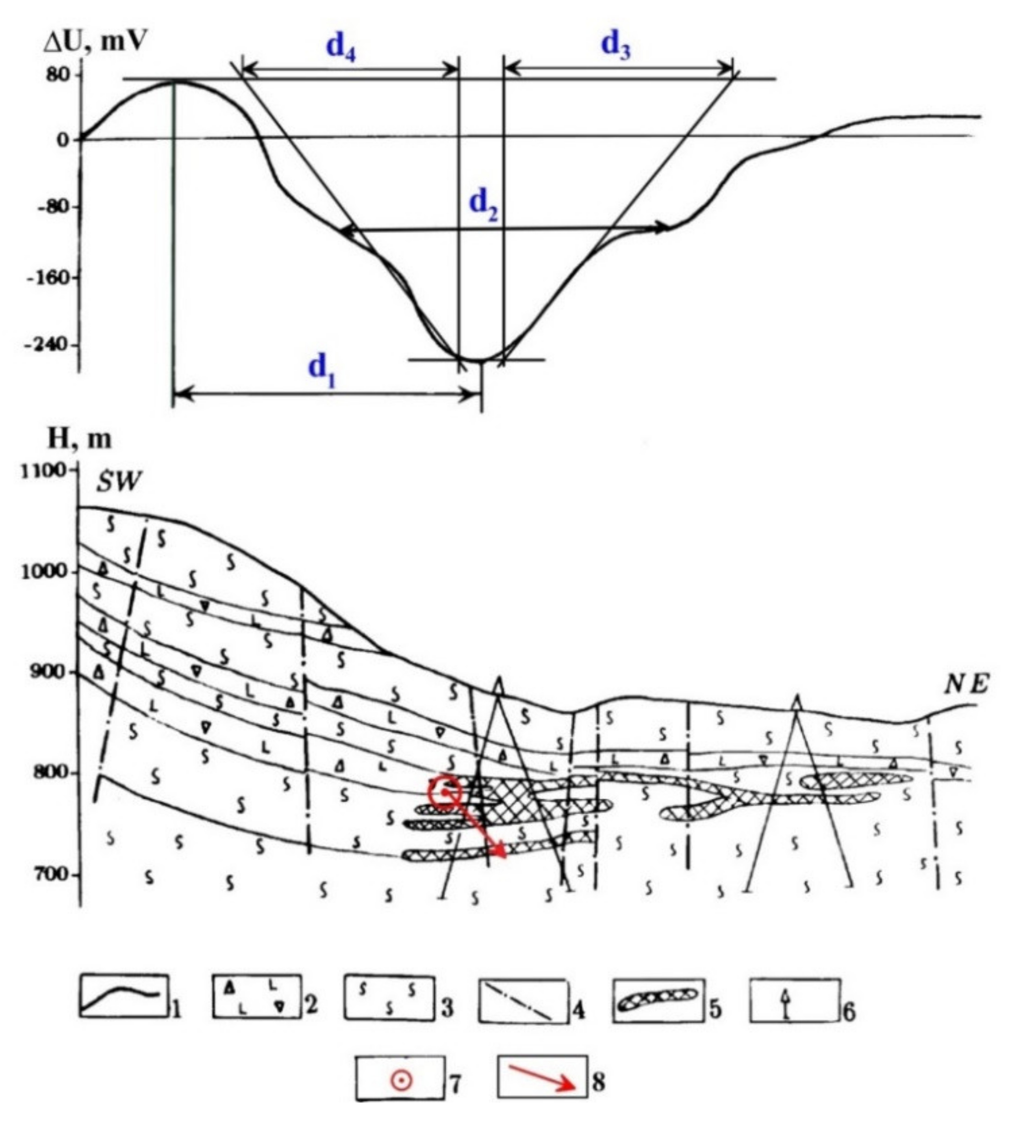
5. Quantitative Analysis of SP Anomalies

The developed interpretation system in the SP method is applicable for complex physical-geological conditions (oblique polarization, inclined relief and superposition of SP anomalies of various orders).

5.1. Testing on Theoretical Models

First of all, the aforementioned interpretation methods were successfully tested on the theoretical SP anomalies for models presented in [3,68,83].

5.2. Mining Geophysics

The self-potential method has often been employed in ore deposits of different kinds (e.g., [3,5,6,7,8,9,10,11,12,13,14,63,64,84,85,86,87,88,89,90,91,92,93]).

5.2.1. Chyragdere Sulfur Deposit (Central Azerbaijan)

It is interesting to compare SP studies carried out over the Ghyragdere sulfur deposit (central Azerbaijan) during several years: 1930, 1937 and 1938 (Figure 4).

This figure shows that the mining works in the underground shaft (1930, 1937 and 1938) strongly distort the SP field observed at the earth’s surface (distance from the observation points to ore deposit consisted several tens of meters). This testifies to the tight correlation between the mining processes and SP anomalies. It would be fascinating to separately compare the volumes and contours of the mined ore with the SP isolines for the abovementioned years, but these documents have been lost over the past years.

5.2.2. Sariyer Sulphide-Pyrite Deposit (Near Istanbul, Turkey)

Yüngül [85] documented the results of the survey in the Sariyer area (Istanbul). The performed interpretation indicates that the obtained position of HCC center is in the line with geometrical and physical parameters of the sulphide-pyrite ore body (Figure 5). Here and in some other figures, displayed parameters d₃ and d₄ relate to the improved tangent method (this method is described in detail, for instance, in [81]). Calculating the self-potential moment by the use of Equations (19b) and (20), we obtain $M_{\mathrm{\Delta }U}=31,800 \mathrm{mV}\cdot {\mathrm{m}}^2.$ This value testifies an intermediate size of the ore body. The calculated direction of self-potential vector by use of Equation (18) is a vertical one.

5.2.3. Polymetallic Deposit (Russia)

Figure 6 displays results of SP anomaly quantitative interpretation using characteristic points and tangent methods (areal method based on the calculation of the area occupied by the SP anomaly has also been applied). The interpretation results, as can easily see from Figure 6, have a good agreement with the location of the ore body. The self-potential moment (here, a model of thin bed was selected and Equations (19a) and (20) were applied) $M_{\mathrm{\Delta }U}=\frac{1}{2}60 \mathrm{mV}\cdot 6.5 \mathrm{m}\cdot 0.93=181 \mathrm{mV}\cdot \mathrm{m}.$ The obtained value indicates the small size of the hidden ore body. The calculated direction of self-potential vector (Equation (18)) roughly corresponds to the dipping of the ore body (Figure 6).

5.2.4. Katsdag Polymetallic Deposit (Azerbaijan)

Three SP anomalies were successfully interpreted in the Katsdag copper-polymetallic deposit (southern slope of the Greater Caucasus, Azerbaijan) under conditions of rugged terrain relief (Figure 7). Anomalies 1 and 2 are intensive ones, but anomaly 3 is comparatively small. It is important to underline here an essential difference between the quantitative results of SP anomalies analysis calculated without and with estimation of the rugged relief influence. The interpretation results are shown for anomalies 1—3 (Figure 7), but the SP moment is calculated only for anomaly 1 (after applying Equations (19a) and (20)) is $M_{\mathrm{\Delta }U}=\frac{1}{2}180 \mathrm{mV}\cdot 20 \mathrm{m}\cdot 0.984=3450 \mathrm{mV}\cdot \mathrm{m}.$ This value indicates an average size of the buried ore body.

5.2.5. Filizchai Polymetallic Deposit (Azerbaijan)

A very intensive SP anomaly (almost 500 mV) was observed in the portion of Filizchai copper-polymetallic field (southern slope of the Greater Caucasus, Azerbaijan) under the conditions of highly complex terrain relief (Figure 8). The results of the interpretation (improved methods of characteristic points and tangents to the thin bed interpretation model were applied) also indicate significant difference of position of the anomalous body calculated without rugged terrain relief influence (blue circle) and after the calculation of this influence (red circle). The calculated SP moment (after Equation (19a)) is $M_{\mathrm{\Delta }U}=\frac{1}{2}440 \mathrm{mV}\cdot 90 \mathrm{m}=19,800 \mathrm{mV}\cdot \mathrm{m}.$ The employment of Equation (20) gives us some decreased value: 14,600 mV·m. It is a sufficiently high value of the SP moment, showing the presence of a large ore body. However, such large SP anomalies of ore origin are rarely observed. The direction of the self-potential vector was calculated by the use of Equation (18). The position of this vector agrees well with the dipping of this pyrite-polymetallic body (Figure 8).

5.2.6. Uchambo Ore Field (Georgia)

Figure 9 depicts the position of the HCC center (characteristic point, tangent and areal methods were applied), which evidently fixes the edge of a flat-lying orebody in the Uchambo polymetallic deposit (southern Georgia). The SP moment calculated using Equations (19b) and (20) is $M_{\mathrm{\Delta }U}=13,480 \mathrm{mV}\cdot {\mathrm{m}}^2.$ This value refers to the lower boundary of the intermediate ore bodies. The complex form of the ore body obviously did not allow for the determination of an exact position of the self-potential vector.

5.2.7. Potentsialnoe Polymetallic Deposit (Rudnyi Altai, Russia)

Here, three different interpreting models were utilized (thin bed, HCC and thick bed) (Figure 10). All three applied models are suitable ones. The calculated SP moment (for HCC model) is (after employing Equations (19b) and (20)) $M_{\mathrm{\Delta }U}=21,890 \mathrm{mV}\cdot {\mathrm{m}}^2.$ This value corresponds to the intermediate ore bodies. The calculated position of the polarization vector (HCC model) coincides with the dipping of the polymetallic body (Figure 10).

5.2.8. Canyon Makhtesh Ramon (Negev Desert, Southern Israel)

The Makhtesh Ramon erosional–tectonic depression (canyon), 40 km long and approximately 8-km wide, is situated in the Negev Desert (southern Israel), 65 km southwest of the Dead Sea. On the basis of integrated geological-geophysical investigations in this area several tens of microdiamonds (largest sample is 1.35 mm) and a large amount of the mineral-satellites of diamond were detected [96]. Many geological-geophysical indicators showed that at least a part of the indigenous sources (kimberlites or lamproites) of the aforementioned minerals can occur in subsurface in this area. The compiled SP map (Figure 11a) displayed the presence of some anomalous zones. Quantitative analysis of the SP anomaly was carried out along profile A—B (Figure 11b) crossing one of the mentioned zones. Results of the performed interpretation indicated that the anomalous inclined body (having a geometrical form close to the thin bed model) occurred at the depth of 40 m, which agrees with the preliminary available geophysical data.

5.3. Archaeological Sites

SP measurements are not frequently applied for searching and localization of archaeological targets, e.g., [15,16,17,18,19,20,21,22,23,97,98]. Obviously, weak SP anomalies and different kinds of noise make it difficult to widely use the self-potential method in archaeological prospection.

The territory of Israel contains more than 35,000 discovered archaeological sites of different age and origin. For SP observations, several typical archaeological sites located in different areas of the country were selected [18,99]. All SP measurements were performed using microvoltmeter with high input impedance and distinctive non-polarizable electrodes (Cu in CuSO₄ solution). The interpretation results obtained earlier at these sites were revised and generalized (the unified methodologies were employed) [100].

5.3.1. Roman Site of Banias (Northern Continuation) (Northern Israel)

The remains of the city of Banias are located in northern Israel at the foot of Mt. Hermon. Banias was the principal city of the Golan and Batanaea regions in the Roman period and occupied an area of more than 250 acres [101]. Here, different ancient remains of Roman and other historical periods were found. The area of the present study is located several km north of the well-investigated Banias site. In the nearest vicinity of the area of geophysical examination (SP and magnetic surveys), the remains of an ancient Roman cemetery and aqueduct were discovered [102]. Mineralogical and geochemical analyses of the excavated Roman chambers indicated that these objects were composed from the special type of hot-worked limestone.

SP observations were carried out by the grid of 1 × 1 m. The compiled SP map (Figure 12) nicely indicates two anomalies. Interpretation profiles I—I and II—II cross the centers of these anomalies (Figure 13). The Upper edges of the recognized anomalous targets occur at the depth of 1.1–1.3 m. Presence of these anomalous sources was confirmed by a comprehensive magnetic data analysis. Angle φ_p for anomaly I consists of 75°, but it is calculated from the opposite side (due to inversion of parameters d₃ and d₄). SP moment for the anomaly I (thin bed) is $M_{\mathrm{\Delta }U}=\frac{1}{2}16.5 \mathrm{mV}\cdot 1.2 \mathrm{m}=9.9 \mathrm{mV}\cdot \mathrm{m}.$ Interestingly, this SP moment is almost 1500 times smaller than the same parameter calculated for the giant SP anomaly in the Filizchai deposit, Azerbaijan (see Figure 8). Such large differences in the aforementioned SP moments is caused by significant differences in the size of these anomalous targets and their electrochemical parameters. For anomaly II, taking into account that parameters d₃ and d₄ are practically equal (θ ≈ 0), the value of polarization angle φ_p is close to 90°. SP moment for anomaly II (HCC) is $M_{\mathrm{\Delta }U}=\frac{2.79 {\mathrm{m}}^2\cdot 18 \mathrm{mV}}{2.6\cdot \cos {15}^{\mathrm{o}}}\cong 20 \mathrm{mV}\cdot {\mathrm{m}}^2.$

5.3.2. Nabatean Site of Halutza (Southern Israel)

The Halutza site is located 20 km southwest of the city of Be’er-Sheva (southern Israel). It was the central city of southern Palestine in the Roman and Byzantine periods and was founded as a way-station for Nabatean (7th–2nd centuries BC) traders traveling between Petra (Jordan) and Gaza. This site was occupied mainly throughout the Byzantine period (4th–7th centuries AD) [103,104].

At this site, self-potential and magnetic measurements were carried out in a 20 × 10 m area with a 1 × 1 m grid [18]. The buried targets (ancient Roman limestone constructions) have produced negative anomalies in both geophysical potential fields. The results of the quantitative examination (here interpretation models of thin bed were utilized) are practically identical (Figure 14A,B). Amplitude of SP anomaly reached 40 mV and is the largest from the anomalies considered in this site. The depth of both of these anomalous targets is about 0.85 m. The calculated moment for the self-potential anomaly is $M_{\mathrm{\Delta }U}=20 \mathrm{mV}\cdot \mathrm{m}.$ The φ_p angle is calculated from the opposite side and consists of 70° (Figure 14B). It may be concluded that the recognized anomalous target approximated by thin bed in the SP method has no vertical dipping, but coinciding with the φ_p angle. The obtained quantitative parameters of ancient constructions agree with the results of archaeological excavations performed in the vicinity of this site.

5.3.3. Christian Site of Emmaus-Nikopolis (Central Israel)

The Christian archaeological site, Emmaus-Nikopolis, is well known in ancient and Biblical history. The site is situated roughly halfway between Jerusalem and Tel Aviv (central Israel). The Crusaders rebuilt it on a smaller scale in the 12th century [101]. Nikopolis is displayed in almost all Christian Pilgrim texts from the fourth century onward; a majority of archaeological sources of this site are named as Emmaus-Nikopolis. Many scientists note that this site is characterized by a multilayer sequence, e.g., [104].

SP measurements in this site were performed by the grid of 1 × 1.5 m. In the compiled SP map (Figure 15), one local anomaly was selected for quantitative analysis (Profile A—B in Figure 15). The determined depth of the target upper edge is about 1.5 m (depth of the HCC center is about 2.1 m) (Figure 16). The φ_p angle consists here of 85° and is calculated from the opposite side.

The self-potential moment of this anomaly (HCC model is employed) consists of 4.5 mV·m². This low value is mainly caused by the small depth and size of the cave. Fragments of some of the glass vessels discovered in this burial cave allowed for it to be attributed to the Byzantine period. Interestingly, to note that magnetic field examination allowed for the recognition in the same cave by the integrated effect from several small magnetic anomalies produced a glass vessel (made from fired clay) [13].

5.4. Environmental Geophysics

Other SP applications revealed such environmental phenomena as karst cavities, faults and rockslides e.g., [24,25,26,27,29,30,31,105,106,107,108,109,110,111,112,113,114].

5.4.1. Buried Cavities in Dolomitic Limestone (Southern Italy)

Several impressive examples of SP application for the detection of underground cavities in southern Italy were displayed in [25]. Let us consider one of these field cases, where buried karst cavity exists in dolomitic limestones (Figure 17). The cavity is horizontally extended and a significant SP anomaly (up to 100 mV) over it was observed. Quantitative examination along profile A—B crossing the center of this anomaly has been performed (Figure 18). For interpretation models of thin bed (upper edge) and center of HCC were obtained depths of 6.0 and 9.5 m, respectively. The self-potential vector is oriented near-vertically. Self-potential moment of anomaly from this cave is about $3300 \mathrm{mV}\cdot {\mathrm{m}}^2$.

5.4.2. Cavities in the Djuanda Forest Park (Bandung, Indonesia)

The next example displays the results of SP and electric resistivity observations carried out above cavities (built during the WW II in early 1940s) at the Djuanda Forest Park, Bandung, Indonesia. Fascinatingly, the resistivity section (Figure 19B) nicely shows two bright anomalies whereas the SP graph (Figure 19A) indicates a significant anomaly (amplitude is more than 20 mV) over cave II, whereas the anomaly over cave I is only emerging (its amplitude is about 2 mV). Obviously, this fact is associated with the hydrogeological peculiarities of the geological section of the subsurface. Quantitative analysis of SP over cave II (here, an interpretation model of thin bed was applied) gave satisfactory results generally coinciding with the results of resistivity section. Calculated self-potential moment here is $M_{\mathrm{\Delta }U}=52 \mathrm{mV}\cdot \mathrm{m}.$

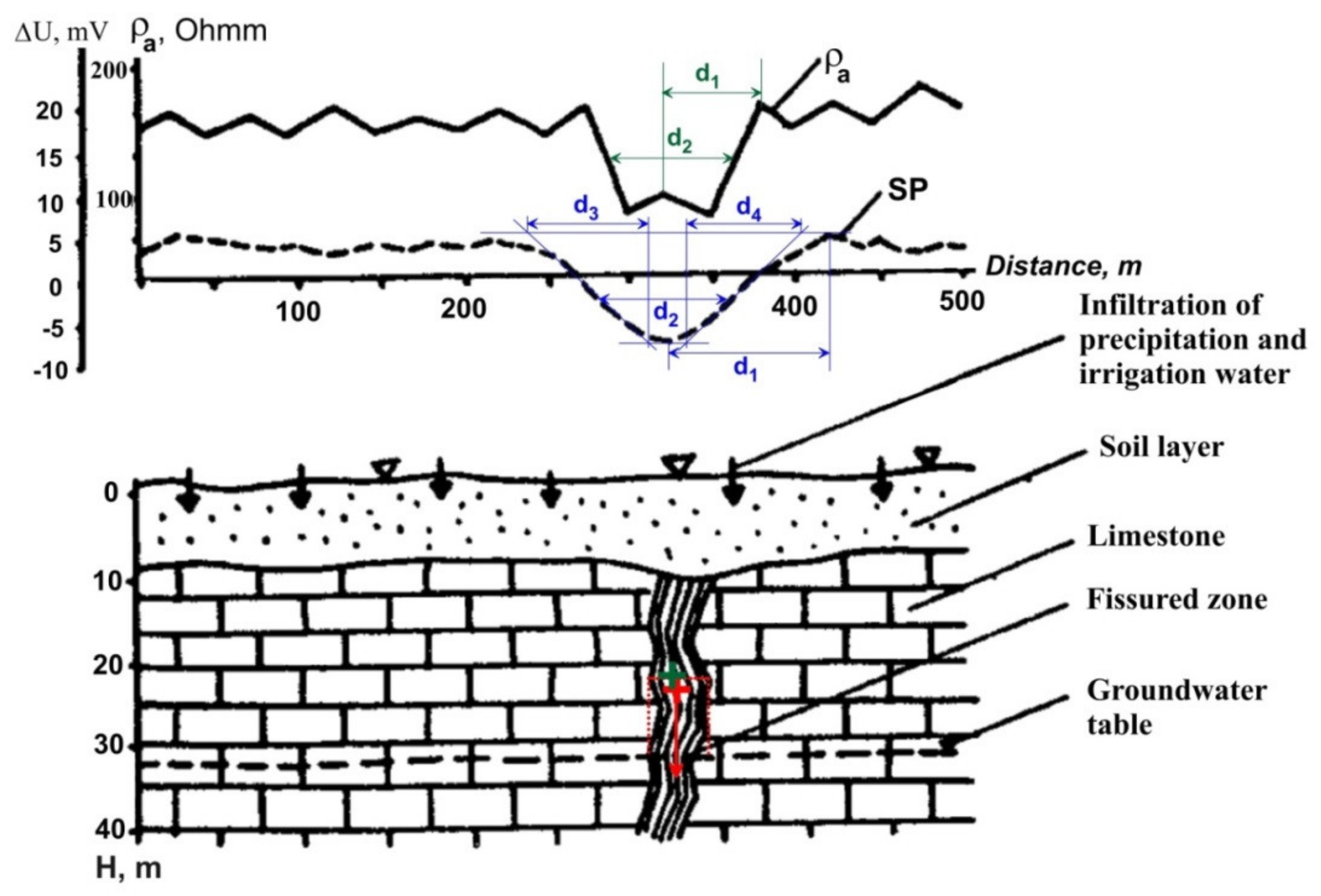
5.4.3. Subvertical Fissure Zone (Russia)

Figure 20 displays the SP and resistivity graphs over the subvertical-fissured zone. SP quantitative examination showed significant disagreement between the results of interpretation and the available geological section. However, it is interesting to note that the performed quantitative analysis of the resistivity curve ρa (presented in the upper part of Figure 20) by the use of the same methodology gave similar results. Theoretical possibilities of such an analysis were reported in Eppelbaum [27] and evaluated in Eppelbaum [13]. Shevnin [115] also indicated a good correlation between the SP and resistivity methods.

Obviously, the disagreement can be explained by some erosion of the upper part of anomalous body (fissured zone) and corresponding changes of its physical properties (possibly appearing to be close to the physical properties of the host media). Nevertheless, the orientation of the self-potential vector coincides with the fissured zone dipping (Figure 20). The value of the self-potential moment (model of thin bed was used) is estimated as $M_{\mathrm{\Delta }U}=23 \mathrm{mV}\cdot \mathrm{m}.$ The low value of the SP moment apparently reflects a small electrochemical ratio of the ‘anomalous target/surrounding medium’.

5.5. Technogenic Geophysics

Let us designate technogenic geophysics as geophysical studies applied to the detection or determination of certain parameters of hidden modern industrial objects. The SP method fits well in such studies.

Onojasun and Takum [34] successfully applied SP investigations for the localization of an underground concrete water pipeline at the Kwinana industrial area of Southern Perth (Western Australia). A comprehensive examination of SP imaging over a metallic contamination plume was performed in [35]. The authors concluded that the SP method can be successfully used to monitor the underground metallic contaminants.

It was established that the examination of SP anomalies is significant for the localization of corrosion in buried oil, gas and water pipes, e.g., [31,32,106,116,117].

Underground Metallic Water-Pipe (Southern Russia)

Fomenko [33] presented a case of a typical SP field distribution over the buried metallic water-pipe (Figure 21). This anomaly has been interpreted by the use of tangent and characteristic point methods. The obtained position of the HCC center agrees (with some assumption) with a center of the hidden water-pipe. The calculated self-potential moment $M_{\mathrm{\Delta }U}=79.8 \mathrm{mV}\cdot {\mathrm{m}}^2.$

5.6. Generalization of the Calculated Self-Potential Moments

The calculated self-potential moments for the variety of studied targets are compiled in

Table 5. Comparison of self-potential moments calculated from different anomalous targets (considered in Section 5.2, Section 5.3, Section 5.4 and Section 5.5).

Object	Location	Approximation Model	Value of Self-Potential Moment $M_{\mathrm{\Delta }U}$
I. Ore geophysics
Sariyer sulphide-pyrite deposit	near Istanbul, Turkey	HCC	$31,800 \mathrm{mV}\cdot {\mathrm{m}}^2$
Polymetallic deposit	Russia	thin bed	$181 \mathrm{mV}\cdot \mathrm{m}$
Katsdag polymetallic deposit	Southern Greater Caucasus, Azerbaijan	thin bed	$3450 \mathrm{mV}\cdot \mathrm{m}$
Filizchai polymetallic deposit (Azerbaijan)	Southern Greater Caucasus, Azerbaijan	thin bed	14,600 mV·m
Uchambo ore field	Lesser Caucasus, Georgia	HCC	$13,480 \mathrm{mV}\cdot {\mathrm{m}}^2$
Potentsialnoe polymetallic deposit	Rudnyi Altai, Russia	thin bed, thick bed, HCC	$21,890 \mathrm{mV}\cdot {\mathrm{m}}^2$ (for HCC)
II. Archaeogeophysics
Banias (anomaly I)	northern Israel	thin bed	$9.9 \mathrm{mV}\cdot \mathrm{m}$
Banias (anomaly II)	“—”	HCC	$20 \mathrm{mV}\cdot {\mathrm{m}}^2$
Halutza	southern Israel	thin bed	$20 \mathrm{mV}\cdot \mathrm{m}$
Emmaus-Nikopolis	central Israel	HCC	4.5 mV·m2
III. Environmental Geophysics
Underground cave	southern Italy	HCC	$3300 \mathrm{mV}\cdot {\mathrm{m}}^2$
Underground cave	Bandung, Indonesia	thin bed	$52 \mathrm{mV}\cdot \mathrm{m}$
Fissured zone	Russia	thin bed	$23 \mathrm{mV}\cdot \mathrm{m}$
IV. Technogenic geophysics
Underground metallic water-pipe	southern Russia	HCC	$79.8 \mathrm{mV}\cdot {\mathrm{m}}^2$

.

The values of self-potential moments presented in Table 5 demonstrate a wide range of the parameters calculated for the models of thin bed and horizontal circular cylinder. $M_{\mathrm{\Delta }U}$ values can be divided in three groups: (1) comparatively large values corresponding to comparatively big ore bodies, (2) middle values relating to targets studying in environmental and technogenic geophysics, and (3) relatively small values reflecting archaeological targets. However, even the smallest $M_{\mathrm{\Delta }U}$ value calculated, for instance, for the ancient cave in the site of Emmaus-Nikopolis, has independent importance.

6. Conclusions

The self-potential method is one of the oldest and simultaneously non-expensive geophysical methods. One of its main preferences is that the presence of water in the subsurface does not limit its method capabilities. The various disturbances complicated the SP observations under different physical-geological environments are analyzed. The available interpretation methodologies are briefly discussed. The proved common aspects between the magnetic and self-potential fields enable for the interpretation of SP anomalies in the modern interpretive procedures developed for complicated environments in magnetic prospecting (oblique magnetization (polarization), rugged topography and an unknown level of the normal field). An explanation of these procedures was presented in detail.

These interpretation procedures applied for SP anomalies enable reliably geometric parameters to be obtained of buried, anomalous targets occurring in complex physical-geological environments. The suggested calculation of direction of the self-polarization vector allows to estimate, in many cases, the dipping of anomalous objects. The proposed calculation of the self-potential moment can be used for the classification of the observed SP anomalies. Testing these procedures in numerous cases of mining, environmental, archaeological and technogenic geophysics in various regions of the world indicates the high practical effectiveness of these developed methodologies.

References

1. Sato, M.; Mooney, H.M. The electrochemical mechanism of sulfide self-potentials. Geophysics 1960, 25, 226–249. [Google Scholar] [CrossRef]
2. Fox, R.W. On the electromagnetic properties of metalliferous veins in the mines of Cornwall. R. Soc. Philos. Trans. 1833, 2, 399–414. [Google Scholar]
3. Semenov, A.S. Electric Prospecting by Self-Potential Method, 4th ed.; revised and supplemented; Nedra: Leningrad, Russia, 1980. (In Russian) [Google Scholar]
4. Parasnis, D.S. Principles of Applied Geophysics, 4th ed.; revised and supplemented; Chapman & Hall: London, UK, 1986. [Google Scholar]
5. Corry, C.E. Spontaneous polarization associated with porphyry sulfide mineralization. Geophysics 1985, 50. [Google Scholar] [CrossRef] [Green Version]
6. Babu, R.H.V.; Rao, A.D. Inversion of self-potential anomalies in mineral exploration. Comput. Geosci. 1988, 14, 377–387. [Google Scholar] [CrossRef]
7. Lile, O.B. Self potential anomaly over a sulphide conductor tested for use as a current source. J. Appl. Geophys. 1996, 36, 97–104. [Google Scholar] [CrossRef]
8. Goldie, M. Self-potentials associated with the Yanacocha high-sulfidation gold deposit in Peru. Geophysics 2002, 67, 684–689. [Google Scholar] [CrossRef]
9. Bhattacharya, B.B.; Shalivakhan, J.A.; Bera, A. Three-dimensional probability tomography of self-potential anomalies of graphite and sulphide mineralization in Orissa and Rajasthan, India. First Break 2007, 5, 223–230. [Google Scholar] [CrossRef]
10. Dmitriev, A.N. Direct and inverse SP modeling on the basis of exact model of self-potential field nature. Geol. Geophys. 2012, 53, 797–812. [Google Scholar] [CrossRef]
11. Fedi, M.; Abbas, M. A fast interpretation of self-potential data using the depth from extreme points method. Geophysics 2013, 78, E107–E116. [Google Scholar] [CrossRef]
12. Biswas, A.; Sharma, S.P. Integrated geophysical studies to elicit the structure associated with uranium mineralization around South Purulia shear zone, India: A review. Ore Geol. Rev. 2016, 72, 1307–1326. [Google Scholar] [CrossRef]
13. Eppelbaum, L.V. Geophysical Potential Fields: Geological and Environmental Applications; Elsevier: Amsterdam, The Netherlands; New York, NY, USA, 2019. [Google Scholar]
14. Eppelbaum, L.V. Advanced system of self-potential field analysis in ore deposits of the South Caucasus. Proc. Natl. Azerbaijan Acad. Sci. 2019, 2, 21–35. [Google Scholar] [CrossRef]
15. Wynn, J.C.; Sherwood, S.I. The self-potential (SP) method: An inexpensive reconnaissance and archaeological mapping tool. J. Field Archaeol. 1984, 11, 195–204. [Google Scholar] [CrossRef]
16. Mauriello, P.; Monna, D.; Patella, D. 3D geoelectric tomography and archaeological applications. Geophys. Prospect. 1998, 46, 543–570. [Google Scholar] [CrossRef]
17. Eppelbaum, L.; Ben-Avraham, Z.; Itkis, S. Ancient Roman remains in Israel provide a challenge for physical-archaeological modeling techniques. First Break 2003, 21, 51–61. [Google Scholar] [CrossRef]
18. Eppelbaum, L.V.; Ben-Avraham, Z.; Itkis, S.E. Integrated geophysical investigations at the Halutza archaeological site. In Proceedings of the 64 EAGE Conference, Florence, Italy, 27–30 May 2002; pp. 1–4. [Google Scholar] [CrossRef]
19. Drahor, M.G. Application of the self-potential method to archaeological prospection: Some case histories. Archaeol. Prospect. 2004, 11, 77–105. [Google Scholar] [CrossRef]
20. Di Maio, R.; Fedi, M.; Lamanna, M.; Grimaldi, M.; Pappaladro, U. The Contribution of Geophysical Prospecting in the Reconstruction of the Buried Ancient Environments of the House of Marcus Fabius Rufus (Pompeii, Italy). Archaeol. Prospect. 2010, 17, 259–269. [Google Scholar] [CrossRef]
21. Shevnin, V.A.; Bobachev, A.A.; Ivanova, S.V.; Baranchuk, K.I. Joint analysis of self potential and electrical resistivity tomography data for studying Alexandrovsky settlement. In Proceedings of the 20th European Meeting of Environmental and Engineering Geophysics, Athens, Greece, 14–18 September 2014; pp. 1–5. [Google Scholar] [CrossRef]
22. De Giorgi, L.; Leucci, G. The archaeological site of Sagalassos (Turkey): Exploring the mysteries of the invisible layers using geophysical methods. Explor. Geophys. 2017, 49, 751–761. [Google Scholar] [CrossRef]
23. De Giorgi, L.; Leucci, G. Passive and Active Electric Methods: New Frontiers of Application. In Innovation in Near-Surface Geophysics; Persico, R., Piro, S., Linford, N., Eds.; Elsevier: Amsterdam, The Netherlands, 2019; pp. 1–21. [Google Scholar] [CrossRef]
24. Corwin, R.F. Application of the Self-Potential Method for Engineering and Environmental Investigations. In SAGEEP Proceedings; Society of Exploration Geophysicists: Tulsa, OK, USA, 1990; pp. 107–121. [Google Scholar]
25. Quarto, R.; Schiavone, D. Detection of cavities by the self-potential method. First Break 1996, 14, 419–430. [Google Scholar] [CrossRef]
26. Jardani, A.; Dupont, J.; Revil, A. Self-potential signals associated with preferential groundwater flow pathways in sinkholes. J. Geophys. Res. 2006, 111, B09204. [Google Scholar] [CrossRef] [Green Version]
27. Eppelbaum, L.V. Revealing of subterranean karst using modern analysis of potential and quasi-potential fields. In Proceedings of the 2007 SAGEEP Conference, Denver, CO, USA, 1–5 April 2007; pp. 797–810. [Google Scholar] [CrossRef]
28. Srigutomo, W.; Arkanuddin, M.R.; Pratomo, P.M.; Novana, E.C.; Agustina, R.D. Application of qualitative and quantitative analyses of self potential anomaly in caves detection in Djuanda Forest Park, Bandung. Am. Inst. Phys. Proc. 2010, 1325, 164–167. [Google Scholar] [CrossRef]
29. Chen, Y.; Qin, X.; Huang, Q.; Gan, F.; Han, K.; Zheng, Z.; Meng, Y. Anomalous spontaneous electrical potential characteristics of epi-karst in the Longrui Depression, Southern Guangxi Province, China. Environ. Earth Sci. 2018, 77, 1–9. [Google Scholar] [CrossRef]
30. Gusev, A.P.; Kaleichik, P.A.; Fedorsky, M.S.; Shavrin, I.A. Dynamics of self-potential field as indicator of dangerous rock-slide areas in industrial landscape (on example of Belarus). Bull. Perm Univ. 2018, 17, 120–127. (In Russian) [Google Scholar]
31. Oliveti, I.; Cardarelli, E. Self-Potential data inversion for environmental and hydrogeological investigations. Pure Appl. Geophys. 2019, 176, 3607–3628. [Google Scholar] [CrossRef]
32. Castermant, J.; Mendonça, C.; Revil, A.; Trolard, F.; Bourrie, G.; Linde, N. Redox potential distribution inferred from self-potential measurements associated with the corrosion of a burden metallic body. Geophys. Prospect. 2008, 56, 269–282. [Google Scholar] [CrossRef]
33. Fomenko, N.E. Ecological Geophysics; South State University: Rostov-on-Don, Russia, 2010. (In Russian) [Google Scholar]
34. Onojasun, O.E.; Takum, E. Geophysical investigation using self-potential techniques: A case of locating underground water pipeline at Kwinana industrial area, Perth. Afr. J. Geo-Sci. Res. 2015, 3, 19–23. [Google Scholar]
35. Cui, Y.; Zhu, X.; Wei, W.; Liu, J.; Tong, T. Dynamic imaging of metallic contamination plume based on self-potential data. Trans. Nonferrous Met. Soc. China 2017, 27, 1822–1830. [Google Scholar] [CrossRef]
36. Perrier, F.; Pant, S.R. Noise reduction in long-term self-potential monitoring with travelling electrode referencing. Pure Appl. Geophys. 2005, 162, 165–179. [Google Scholar] [CrossRef]
37. Zaborovsky, A.I. Electric Prospecting; Gostoptekhizdat: Moscow, Russia, 1963. (In Russian) [Google Scholar]
38. Khesin, B.E.; Alexeyev, V.V.; Eppelbaum, L.V. Interpretation of Geophysical Fields in Complicated Environments; Modern Approaches in Geophysics, Boston–Dordrecht–London; Kluwer Academic Publishers (Springer): Amsterdam, The Netherlands, 1996. [Google Scholar]
39. Ernstson, K.; Scherer, V. Self-potential variations with time and their relation to hydrogeologic and meteorological parameters. Geophysics 1986, 51, 1967–1977. [Google Scholar] [CrossRef]
40. Eppelbaum, L.V.; Mishne, A.R. Unmanned Airborne Magnetic and VLF investigations: Effective Geophysical Methodology of the Near Future. Positioning 2011, 2, 112–133. [Google Scholar] [CrossRef] [Green Version]
41. Wang, J.-H.; Geng, Y. Terrain correction in the gradient calculation of spontaneous potential data. Chin. J. Geophys. 2015, 58, 654–664. [Google Scholar] [CrossRef]
42. Telford, W.M.; Geldart, L.P.; Sheriff, R.E. Applied Geophysics, 2nd ed.; Cambridge University Press: Cambridge, UK, 1990. [Google Scholar]
43. Revil, A.; Jardani, A. The Self-Potential Method: Theory and Applications in Environmental Geosciences; Cambridge University Press: Cambridge, UK, 2013. [Google Scholar]
44. Perrier, F.; Morat, P. Characterization of electrical daily variations induced by capillary flow in the non-saturated zone. Pure Appl. Geophys. 2000, 157, 785–810. [Google Scholar] [CrossRef]
45. Jardani, A.; Revil, A. Stochastic joint inversion of temperature and self-potential data. Geophys. J. Int. 2009, 179, 640–654. [Google Scholar] [CrossRef] [Green Version]
46. Petrovsky, A. The problem of a hidden polarized sphere. Philos. Mag. 1928, 5, 914–933. [Google Scholar] [CrossRef]
47. Murty, B.V.; Haricharan, P. A simple approach toward interpretation SP anomaly due to 2-D sheet model of short dipole length. Geophys. Res. Bull. 1984, 22, 213–218. [Google Scholar]
48. Fitterman, D.V. Calculation of self-potential anomalies near vertical contacts. Geophysics 1979, 44, 195–205. [Google Scholar] [CrossRef]
49. Rao, D.A.; Babu, H.V.; Sivakumar, G.D.J. A Fourier transform method for the interpretation of SP anomalies due to two-dimensional inclined sheets of finite depth extent. Pure Appl. Geophys. 1982, 120, 365–374. [Google Scholar] [CrossRef]
50. Rao, S.V.S.; Mohan, N.L. Spectral interpretation of self-potential anomaly due to an inclined sheet. Curr. Sci. 1984, 53, 474–477. [Google Scholar]
51. Banerjee, B.; Pal, B.P. Frequency domain interpretation of Self-Potential anomalies. Gerlands Beitr. Geophys. 1990, 99, 531–538. [Google Scholar]
52. Skianis, G.A.; Papadopoulos, T.D.; Vaiopoulos, D.A. 1-D and 2-D spatial frequency analysis of SP field anomalies produced by a polarized sphere. Pure Appl. Geophys. 1991, 137, 251–260. [Google Scholar] [CrossRef]
53. Skianis, G.; Papadopoulos, T.; Vaiopoulos, D.A.; Nikolaou, S. A new method of quantitative interpretation of SP anomalies produced by a polarized inclined sheet. Geophys. Prospect. 1995, 43, 677–691. [Google Scholar] [CrossRef]
54. Abdelrahman, E.M.; Sharafeldin, S.M. A least squares approach to depth determination from residual self-potential anomalies caused by horizontal cylinders and spheres. Geophysics 1997, 62, 44–48. [Google Scholar] [CrossRef]
55. Abdelrahman, E.M.; El-Araby, T.M.; Ammar, A.A.; Hassanein, H.I. A least-squares approach to shape determination from selfpotential anomalies. Pure Appl. Geophys. 1997, 150, 121–128. [Google Scholar] [CrossRef]
56. Abdelrahman, E.M.; Ammar, A.A.; Hassanein, H.I.; Hafez, M.A. Derivative analysis of SP anomalies. Geophysics 1998, 63, 890–897. [Google Scholar] [CrossRef]
57. El-Araby, H.M. A new method for complete quantitative interpretation of self-potential anomalies. J. Appl. Geophys. 2004, 55, 211–224. [Google Scholar] [CrossRef]
58. Essa, K.; Mehanee, S.; Smith, P.D. A new inversion algorithm for estimating the best fitting parameters of some geometrically simple body to measured self-potential anomalies. Explor. Geophys. 2008, 39, 155–163. [Google Scholar] [CrossRef]
59. Gibert, D.; Pessel, M. Identification of sources of potential fields with the continuous wavelet transform: Application to SP profiles. Geophys. Res. Lett. 2001, 28, 1863–1866. [Google Scholar] [CrossRef]
60. Sailhac, P.; Marquis, G. Analytic potentials for the forward and inverse modeling of SP anomalies caused by subsurface fluid flow. Geophys. Res. Lett. 2001, 28, 1851–1854. [Google Scholar] [CrossRef] [Green Version]
61. Patella, D. Introduction to ground surface self-potential tomography. Geophys. Prospect. 1997, 45, 653–681. [Google Scholar] [CrossRef]
62. Di Maio, R.; Piegari, E.; Rani, P.; Avella, A. Self-Potential data inversion through the integration of spectral analysis and tomographic approaches. Geophys. J. Int. 2016, 206, 1204–1220. [Google Scholar] [CrossRef]
63. Mendonça, C.A. Forward and inverse self-potential modeling in mineral exploration. Geophysics 2008, 73, F33–F43. [Google Scholar] [CrossRef]
64. Srivastava, S.; Agarwal, B.N.P. Interpretation of self-potential anomalies by enhanced local wave number technique. J. Appl. Geophys. 2009, 68, 259–268. [Google Scholar] [CrossRef]
65. Al-Garni, M.A. Interpretation of spontaneous potential anomalies from some simple geometrically shaped bodies using neural network inversion. Acta Geophys. 2017, 58, 143–162. [Google Scholar] [CrossRef]
66. Hristenko, L.A.; Stepanov, Y.I. Transformation of SP observations for solving engineering-geological problems. Min. Inf. Anal. Bull. 2012, 169–173. (In Russian) [Google Scholar]
67. Gobashy, M.; Abdelazeem, M.; Abdrabou, M.; Khalil, M.H. Estimating model parameters from self-potential anomaly of 2D inclined sheet using whale optimization algorithm: Applications to mineral exploration and tracing shear zones. Nat. Resour. Res. 2020, 29, 499–519. [Google Scholar] [CrossRef]
68. Rao, K.; Jain, S.; Biswas, A. Global optimization for delineation of self-potential anomaly of a 2D inclined plate. Nat. Resour. Res. 2021, 30, 175–189. [Google Scholar] [CrossRef]
69. Tlas, M.; Asfahani, J. An approach for interpretation of self-potential anomalies due to simple geometrical structures using Fair function minimization. Pure Appl. Geophys. 2013, 170, 895–905. [Google Scholar] [CrossRef]
70. Giannakis, I.; Tsourlos, P.; Papazachos, C.; Vargemezis, G.; Giannopoulos, A.; Papadopoulos, N.; Tosti, F.; Alani, A. A hybrid optimization scheme for self-potential measurements due to multiple sheet-like bodies in arbitrary 2D resistivity distributions. Geophys. Prospect. 2019, 67, 1948–1964. [Google Scholar] [CrossRef]
71. Kilty, K.T. On the origin and interpretation of self-potential anomalies. Geophys. Prospect. 1984, 32, 51–62. [Google Scholar] [CrossRef]
72. Eppelbaum, L.V.; Khesin, B.E. Geophysical Studies in the Caucasus; Springer: Heidelberg, Germany; New York, NY, USA, 2012. [Google Scholar]
73. Zhdanov, M.S.; Keller, G.V. The Geoelecrical Methods in Geophysical Exploration; Elsevier: Amsterdam, The Netherlands, 1994. [Google Scholar]
74. Jardani, A.; Revil, A.; Bolève, A.; Dupont, J.P. Three-dimensional inversion of self-potential data used to constrain the pattern of groundwater flow in geothermal fields. J. Geophys. Res. 2008, 113, B09204. [Google Scholar] [CrossRef]
75. Akgün, M. Estimation of some bodies parameters from the self potential method using Hilbert transform. J. Balk. Geophys. Soc. 2001, 4, 29–44. [Google Scholar]
76. Sindirgi, P.; Pamukçu, O.; Özyalin, S. Application of normalized full gradient method to self potential (SP) data. Pure Appl. Geophys. 2008, 165, 409–427. [Google Scholar] [CrossRef]
77. Sindrigi, P.; Özyalin, S. Estimating the location of a causative body from a self-potential anomaly using 2D and 3D normalized full gradient and Euler deconvolution. Turk. J. Earth Sci. 2019, 28, 640–659. [Google Scholar] [CrossRef]
78. Agarwal, B.N.P.; Srivastava, S. Analyses of self-potential anomalies by conventional and extended Euler deconvolution techniques. Comput. Geosci. 2009, 35, 2231–2238. [Google Scholar] [CrossRef]
79. Biswas, A. Inversion of Amplitude from the 2-D Analytic Signal of Self-Potential Anomalies. In Minerals; Essa, K.S., Ed.; IntechOpen: London, UK, 2018; pp. 13–45. [Google Scholar] [CrossRef] [Green Version]
80. Sungkono. Robust interpretation of single and multiple self-potential anomalies via flower pollination algorithm. Arab. J. Geosci. 2020, 13, 1–15. [Google Scholar] [CrossRef]
81. Eppelbaum, L.V.; Khesin, B.E.; Itkis, S.E. Prompt magnetic investigations of archaeological remains in areas of infrastructure development: Israeli experience. Archaeol. Prospect. 2001, 8, 163–185. [Google Scholar] [CrossRef]
82. Eppelbaum, L.V. Quantitative interpretation of magnetic anomalies from bodies approximated by thick bed models in complex environments. Environ. Earth Sci. 2015, 74, 5971–5988. [Google Scholar] [CrossRef]
83. Göktürkler, G.; Balkaya, Ç. Inversion of self-potential anomalies caused by simple-geometry bodies using global optimization algorithms. J. Geophys. Eng. 2012, 10, 498–507. [Google Scholar] [CrossRef]
84. Stern, W. Relation between spontaneous polarization curves and depth, size, and dip of ore bodies. Trans. Am. Inst. Min. Metallurg. Petr. Eng. 1945, 164, 189–196. [Google Scholar]
85. Yüngül, S. Spontaneous-potential survey of a copper deposit at Sariyer, Turkey. Geophysics 1954, 19, 455–458. [Google Scholar] [CrossRef]
86. Sengupta, S.N.; Bose, R.N.; Mitra, S.K. Geophysical investigations for copper ores in the Singhana-Gotpo area, Khetri copper belt, Rajasthan (India). Geoexpoloration 1969, 7, 73–82. [Google Scholar] [CrossRef]
87. Logn, O.; Bolviken, B. Self potentials at the Joma pyrite deposit, Norway. Geoexploration 1974, 12, 11–28. [Google Scholar] [CrossRef]
88. Cowan, D.R.; Allchurch, P.D.; Omnes, G. An integrated geo-electrical survey on the Nangaroo copper-zinc prospect, near Leonora, Western Australia. Geoexploration 1975, 13, 77–98. [Google Scholar] [CrossRef]
89. Nayak, P.N. Electromechanical potential in surveys for sulphide. Geoexploration 1981, 18, 311–320. [Google Scholar] [CrossRef]
90. Alizadeh, A.M.; Guliyev, I.S.; Kadirov, F.A.; Eppelbaum, L.V. Geosciences in Azerbaijan. Volume II: Economic Minerals and Applied Geophysics; Springer: Heidelberg, Germany; New York, NY, USA, 2017. [Google Scholar]
91. Erofeev, L.Y.; Orekhov, A.N.; Erofeeva, G.V. Natural electric fields in Siberian gold deposits: Structure, origin, and relationship with gold orebodies. Geol. Geophys. 2017, 58, 984–989. [Google Scholar] [CrossRef]
92. Safipour, R.; Hölz, S.; Halbach, J.; Jegen, M.; Petersen, S.; Swidinsky, A. A self-potential investigation of submarine massive sulfides, Palinuro Seamount, Tyrrhenian Sea. Geophysics 2017, 82, A51–A56. [Google Scholar] [CrossRef] [Green Version]
93. Zhu, Z.; Shen, J.; Tao, C.; Deng, X.; Wu, T.; Nie, Z.; Wang, W.; Su, Z. Autonomous underwater vehicle based marine multi-component self-potential method: Observation scheme and navigational correction. Geosci. Instrum. Methods Data Syst. 2020, 10, 1–25. [Google Scholar] [CrossRef]
94. Bukhnikashvili, A.V.; Kebuladze, V.V.; Tabagua, G.G.; Dzhashi, G.G.; Gugunava, G.E.; Tatishvili, O.V.; Gogua, R.A. Geophysical Exploration of Adjar Group of Copper-Polymetallic Deposits; Metsniereba: Tbilisi, Russia, 1974. (In Russian) [Google Scholar]
95. Semenov, M.V. Principles of Prospecting and Investigating Pyrite-Polymetallic Ore Fields by Geophysical Methods; Nedra: Leningrad, Russia, 1975. (In Russian) [Google Scholar]
96. Eppelbaum, L.V.; Vaksman, V.L.; Kouznetsov, S.V.; Sazonova, L.M.; Smirnov, S.A.; Surkov, A.V.; Bezlepkin, B.; Katz, Y.; Korotaeva, N.N.; Belovitskaya, G. Discovering of microdiamonds and minerals-satellites in Canyon Makhtesh Ramon (Negev desert, Israel). Dokl. Earth Sci. 2006, 407, 202–204. [Google Scholar] [CrossRef]
97. Drahor, M.G.; Akyol, A.L.; Dilaver, N. An application of the self-potential (SP) method in archaeogeophysical prospection. Archaeol. Prospect. 2006, 3, 141–158. [Google Scholar] [CrossRef]
98. Tsokas, G.N.; Tourlos, P.I.; Kim, J.-H.; Papazachos, C.B.; Vargemezis, G.; Bogiatzis, P. Assessing the condition of the rock mass over the tunnel of Eupalinus in Samos (Greece) using both conventional geophysical methods and surface to tunnel electrical resistivity tomography. Archaeol. Prospect. 2014, 21, 277–291. [Google Scholar] [CrossRef]
99. Eppelbaum, L.V.; Khesin, B.E.; Itkis, S.E.; Ben-Avraham, Z. Advanced analysis of self-potential data in ore deposits and archaeological sites. In Proceedings of the 10th European Meeting of Environmental and Engineering Geophysics, Utrecht, The Netherlands, 6–9 September 2004; pp. 1–4. [Google Scholar] [CrossRef]
100. Eppelbaum, L.V. Quantitative analysis of self-potential anomalies in archaeological sites of Israel: An overview. Environ. Earth Sci. 2020, 79, 1–15. [Google Scholar] [CrossRef]
101. Meyers, E.M. (Ed.) The Oxford Encyclopedia of Archaeology in the Near East; Oxford University Press: Oxford, UK, 1996; Volume 5. [Google Scholar]
102. Hartal, M. Banias, the Aqeduct. Excav. Surv. Isr. 1997, 16, 5–8. [Google Scholar]
103. Kenyon, K.M. Archaeology in the Holy Land; Norton: New York, NY, USA, 1979. [Google Scholar]
104. Kempinski, A.; Reich, R. (Eds.) The Architecture of Ancient Israel; Israel Exploration Society: Jerusalem, Israel, 1992. [Google Scholar]
105. Ogilvy, A.A.; Bogoslovsky, V.A. The possibilities of geophysical methods applied for investigating the impact of man on the geological medium. Geophys. Prospect. 1979, 27, 775–789. [Google Scholar] [CrossRef]
106. Corwin, R.F. The Self-Potential Method for Environmental and Engineering Application. In Geotechnical and Environmental Geophysics; Ward, S.H., Ed.; Society of Exploration Geophysicists: Tulsa, OK, USA, 1996; Volume 1, pp. 127–145. [Google Scholar]
107. Gurk, M.; Bosch, F. Cave detection using the Self-Potential-Surface (SPS) technique on a karstic terrain in the Jura Mountains (Switzerland). In Proceedings of the Kolloquium Elektromagnetische Tiefenforschung, Burg Ludwigstein, Germany, 9–13 March 2001; pp. 283–291. [Google Scholar]
108. Vichabian, Y.; Morgan, F.D. Self-potentials in cave detection. Lead. Edge 2002, 21, 866–871. [Google Scholar] [CrossRef]
109. Lapenna, V.; Lorenzo, P.; Perrone, A.; Piscitelli, S.; Sdao, F.; Rizzo, E. High-resolution geoelectrical tomographies in the study of Giarrossa landslide (southern Italy). Bull. Eng. Geol. Environ. 2003, 62, 259–268. [Google Scholar] [CrossRef]
110. Jardani, A.; Revil, A.; Dupont, J. Self-potential tomography applied to the determination of cavities. Geophys. Res. Lett. 2006, 23, L13401. [Google Scholar] [CrossRef]
111. Jardani, A.; Revil, A.; Santos, F.; Fauchard, C.; Dupont, J. Detection of preferential infiltration pathways in sinkholes using joint inversion of self-potential and EM-34 conductivity data. Geophys. Prospect. 2007, 55, 749–760. [Google Scholar] [CrossRef]
112. Rozycki, A.; Fonticiella, J.M.R.; Cuadra, A. Detection and evaluation of horizontal fractures in Earth dams using self-potential method. Eng. Geol. 2006, 82, 145–153. [Google Scholar] [CrossRef]
113. Gibert, D.; Sailhac, P. Comment on ‘‘Self-potential signals associated with preferential groundwater flow pathways in sinkholes’’ by A. Jardani, J.P. Dupont, and A. Revil, J. of Geophys. Res.; 113, B03210. J. Geophys. Res. 2008, 113, B03210. [Google Scholar] [CrossRef] [Green Version]
114. Tripathi, G.N.; Frayar, A.E. Integrated surface geophysical approach to locate a karst conduit: A case study from Royal Spring Basin, Kentucky, USA. J. Nepal Geol. Soc. 2016, 51, 27–37. [Google Scholar] [CrossRef]
115. Shevnin, V.A. Identification of self-potential anomalies of a diffusion-absorption origin. Mosc. Univ. Geol. Bull. 2018, 73, 306–311. [Google Scholar] [CrossRef]
116. Ekine, A.S.; Emujakporue, G.O. Investigation of corrosion of buried oil pipeline by the electrical geophysical methods. J. Appl. Sci. Environ. Manage. 2010, 14, 63–65. [Google Scholar] [CrossRef]
117. Rittgers, J.B.; Revil, A.; Karaoulis, M.; Mooney, M.A.; Slater, L.D.; Atekwana, E.A. Self-potential signals generated by the corrosion of buried metallic objects with application to contaminant plumes. Geophysics 2013, 78, EN65–EN82. [Google Scholar] [CrossRef]
Figure 1. General scheme of disturbances in SP method (after [14], with modifications).
Geosciences 11 00194 g001
Figure 2. SP observations at inclined relief (after [39], with small modifications) (Middle Keuper of the Steigerwald highlands, 60 km east of Würzburg, Germany).
Geosciences 11 00194 g002
Figure 3. A correlation between temperature and SP observations: (a) temperature, (b) SP intensity, (c) correlation between these parameters (a,b are taken from [39]). SP observations were carried out in the Middle Keuper of the Steigerwald highlands, 60 km east of Würzburg, Germany.
Geosciences 11 00194 g003
Figure 4. Displacement of self-potential isolines during exploitation of the new shaft of Chyragdere sulfur deposit (Lesser Caucasus) (after [72], with modifications). (1) Stock contour, (2) isolines of self-potential field (in millivolts).
Geosciences 11 00194 g004
Figure 5. Quantitative interpretation of SP anomaly by the characteristic point and tangent methods in the Sariyer area, Turkey. The “” symbol marks the obtained position of the ore body center (approximated by a HCC). The red arrow shows the direction of self-polarization vector. Observed SP curve and geological section are taken from [85].
Geosciences 11 00194 g005
Figure 6. Quantitative interpretation of SP anomaly over polymetallic body (Rudnyi Altai, Russia). Observed SP curve and geological section ((1)–(5)) are taken from [3,37]. (1) limestone, (2) shales, (3) copper-polymetallic ore body, SP observations carried out in (4) 1952 and (5) 1953, (6) determined position of the center of the upper edge of the ore body, (7) direction of the self-potential vector.
Geosciences 11 00194 g006
Figure 7. Results of the quantitative interpretation of SP anomalies in the area of the Katsdagh copper-polymetallic deposits on the southern slope of the Greater Caucasus (Azerbaijan). (1) Interbedding of sands and clay schists, (2) clay schists with the flysh packages, (3) clay sandstone; (4) sand-clay schists; (5) diabases, gabbro-diabases and diabasic porphyrites; (6) andesites and andesite-porphyrites; (7) dacitic porphyrites; (8) faults; (9) massive ore of pyrite-polymetallic composition; (10) oxidized ore; (11) zones of brecciation, crush and boudinage with lean pyrite-polymetallic ore; (12) SP curves; location of anomalous source: (13) without calculation of the inclined relief influence, (14) after introducing correction for the terrain relief, (15) direction of the self-potential vector.
Geosciences 11 00194 g007
Figure 8. Results of quantitative interpretation of SP anomaly in the area of Filizchay copper-polymetallic deposit in the southern slope of the Greater Caucasus (Azerbaijan) (revised after [72]). (1) Interbedding of sands and clay schists, (2) clay schists with the flysh packages, (3) clay sandstone, (4) faults, (5) massive ore of pyrite-polymetallic composition, (6) oxidized ore, (7) SP curves, location of anomalous source: (8) without calculation of the inclined relief influence, (9) after introducing correction for the surface relief, (10) direction of the self-potential vector.
Geosciences 11 00194 g008
Figure 9. Interpretation of SP anomaly in the area of the Uchambo ore field of the Adjar group of copper-polymetallic deposits (Georgia, Lesser Caucasus). (1) SP observed values; (2) heteroclastic tuff breccia and their tuffs; (3) cover trachyandesite-basalts with pyroclastic interbeds; (4) disjunctive dislocations; (5) zones of increased mineralization; (6) drilled wells; (7) location of HCC center according to the interpretation results, (8) orientation of self-potential vector (1–6) from [94].
Geosciences 11 00194 g009
Figure 10. Interpretation by the developed techniques of SP anomaly in the area of the Potentsialnoe deposit (Rudny Altai, Russia) (initial data from [95]). (1) Soil-vegetative layer; (2) alternation of lavas and tuffs of acid composition and chlorite-sericitic schists; (3) sulfide ores; (4) sulfide impregnation, pyritization; (5) level of ground waters; (6) drilling wells (a) and adits (b); (7) SP plot; (8) interpretation results: (a) center of the upper edge of the thin bed, (b) mid-point of the inclined thick bed’s upper edge, (c) center of a horizontal circular cylinder (arrow indicates the direction of the polarization vector obtained by interpretation).
Geosciences 11 00194 g010
Figure 11. (a) SP map observed in the area of the western Makhtesh Ramon (northern Negev desert). Line A—B indicates position of the interpreting profile. (b) Interpretation of the SP anomaly along profile A—B, western Makhtesh Ramon (see Figure 11a). The red cross indicates the position of the center of the upper edge of the anomalous body, and the red arrow indicates the orientation of the self-potential vector.
Geosciences 11 00194 g011
Figure 12. Self-potential map observed in the Banias site (northern Israel) and location of interpreting profiles I—I’ and II—II’.
Geosciences 11 00194 g012
Figure 13. Quantitative analysis of anomalies I–I’ and II–II’ (see Figure 12) in the Banias site (northern Israel). The red cross indicates position of the center of upper edge, the bold red point testifies a position of HCC center, and the black arrows show direction of self-polarization vector.
Geosciences 11 00194 g013
Figure 14. Quantitative analysis of magnetic (A) and self-potential (B) anomalies in the site of Halutza (southern Israel). The red cross in both models indicates position of the center of the upper edge, and the red arrow (in B) shows direction of self-polarization vector.
Geosciences 11 00194 g014
Figure 15. Self-potential map observed in the site of Emmaus-Nikopolis (central Israel).
Geosciences 11 00194 g015
Figure 16. Quantitative analysis of self-potential anomaly along profile A–B in the site of Emmaus-Nikopolis (SP map is presented in Figure 15). The black arrow shows the direction of self-polarization vector.
Geosciences 11 00194 g016
Figure 17. SP map over underground cave and position of interpreting profile A—B (SP map after [25]).
Geosciences 11 00194 g017
Figure 18. Quantitative analysis of SP anomaly along profile A—B (location of profile is shown in Figure 17). The red cross designates the position of the middle of the thin bed upper edge, the red circle shows the position of the center of the horizontal circular cylinder (HCC). The black arrow shows the orientation of the polarization vector.
Geosciences 11 00194 g018
Figure 19. Quantitative analysis of SP anomalies over underground caves in the Djuanda Forest Park, Bandung (Indonesia). (A) SP profile with interpretation of anomaly II, (B) ERT section, (C) geological section. Initial data taken from [28]. The white circle and arrow indicate the position of upper edge of cave II and its dipping (distribution of the highest resistivities). Black arrows show corresponding cavities.
Geosciences 11 00194 g019
Figure 20. The interpretation of SP anomaly over the fissured zone (Russia) (resistivity and SP graphs and geological section are from [105]). The red and green crosses show the positions of the upper edge of the anomalous target determined from SP and resistivity curves, respectively. The red arrow indicates the orientation of self-potential vector.
Geosciences 11 00194 g020
Figure 21. Quantitative examination of the SP anomaly from the buried metallic pipe (southern Russia). Observed SP graph and near-surface section are taken from [33]. The red circle indicates the determined position of the center of HCC, and the red arrow shows the orientation of the self-potential vector.
Geosciences 11 00194 g021