Article

Time-Domain Studies of General Dispersive Anisotropic Media by the Complex-Conjugate Pole–Residue Pairs Model

by
Konstantinos P. Prokopidis
1 and
Dimitrios C. Zografopoulos
2,*
1
School of Electrical and Computer Engineering, Aristotle University of Thessaloniki, GR-54124 Thessaloniki, Greece
2
Consiglio Nazionale delle Ricerche, Istituto per la Microelettronica e Microsistemi (CNR-IMM), 00133 Rome, Italy
*
Author to whom correspondence should be addressed.
Appl. Sci. 2021, 11(9), 3844; https://doi.org/10.3390/app11093844
Submission received: 7 April 2021 / Revised: 20 April 2021 / Accepted: 21 April 2021 / Published: 23 April 2021
(This article belongs to the Section Electrical, Electronics and Communications Engineering)

Abstract

:
A novel finite-difference time-domain formulation for the modeling of general anisotropic dispersive media is introduced in this work. The method accounts for fully anisotropic electric or magnetic materials with all elements of the permittivity and permeability tensors being non-zero. In addition, each element shows an arbitrary frequency dispersion described by the complex-conjugate pole–residue pairs model. The efficiency of the technique is demonstrated in benchmark numerical examples involving electromagnetic wave propagation through magnetized plasma, nematic liquid crystals and ferrites.

1. Introduction

The finite-difference time-domain (FDTD) method [1] is widely recognized as one of the dominant tools in computational electromagnetics, particularly in the study of the broadband spectral response of electromagnetic structures. In such large frequency intervals, most materials are dispersive; namely, they exhibit a frequency-dependent variation of their electrical permittivity and magnetic permeability. From the early stages of its development, the FDTD was demonstrated to be capable of accurately simulating the dispersive properties of most common materials, both dielectric and metallic [2].
In several cases involving advanced natural or artificial materials, it is not only their dispersive nature that has to be taken into account but also their anisotropy. This problem has been addressed in various FDTD techniques, which have been proposed for the numerical simulation of certain types of both anisotropic and dispersive media [3,4,5,6,7,8,9].
As concerns the FDTD modeling of dispersive materials, the complex-conjugate pole–residue pairs (CCPR) model, a generalization of the traditional Drude and Lorentz models, has been proven to provide a more accurate description of material dispersion [10,11] with reduced memory requirements and similar conditions for numerical stability [12]. Recently, we have demonstrated how the CCPR can be combined with electric anisotropy for the accurate investigation of nematic liquid crystals (NLC) [13]. The dispersion of the ordinary and extraordinary NLC indices were described by the CCPR model, and the FDTD scheme accounted for both the dispersion and the NLC anisotropy. CCPR modeling has been also combined with implicit FDTD formulations—in particular, the leapfrog alternating-direction implicit FDTD—confirming the robustness of the approach for the accurate description of dispersive materials [14].
In the present work, the CCPR dispersion model is incorporated into an explicit FDTD, which accounts for a generalized form of the permittivity or permeability tensor. All elements of the electric and magnetic tensors are allowed to obtain non-zero values. Moreover, they are allowed to independently exhibit frequency dispersion following the CCPR model with an arbitrary number of terms and are capable of capturing the behavior of dispersive material over broad spectral ranges. The FDTD implementation algorithm is outlined, and the associated generalized update expressions are obtained. The efficiency of the technique is corroborated in benchmark examples studying electromagnetic wave propagation through three types of dispersive and anisotropic materials: (i) magnetized plasma, (ii) NLC and (iii) ferrites. The proposed FDTD scheme provides extensive versatility in the modeling of the arbitrary dispersive characteristics of the tensor elements of anisotropic materials and a robust framework for the study of electromagnetic systems that involve dispersive anisotropic media.

2. Formulation

The time-harmonic Maxwell’s equations in a linear, source-free, electrically and magnetically anisotropic dispersive medium with e j ω t time dependence are as follows:
× E ˜ = j ω μ 0 μ ¯ ¯ ( ω ) H ˜ ,
× H ˜ = j ω ε 0 ε ¯ ¯ ( ω ) E ˜ ,
where the tilde on the fields denotes the frequency domain, and the frequency-dependent relative permittivity tensor ε ¯ ¯ ( ω ) is described by the following general expression:
ε ¯ ¯ ( ω ) = ε x x ( ω ) ε x y ( ω ) ε x z ( ω ) ε y x ( ω ) ε y y ( ω ) ε y z ( ω ) ε z x ( ω ) ε z y ( ω ) ε z z ( ω ) .
Similarly, the relative permeability tensor μ ¯ ¯ ( ω ) is given by
μ ¯ ¯ ( ω ) = μ x x ( ω ) μ x y ( ω ) μ x z ( ω ) μ y x ( ω ) μ y y ( ω ) μ y z ( ω ) μ z x ( ω ) μ z y ( ω ) μ z z ( ω ) .
In this work, we adopt the CCPR model for the description of the dispersive elements ε α β ( ω ) , μ α β ( ω ) . We explicitly present the formulation for electric anisotropic dispersive media, according to which the complex relative permittivity of the tensor elements is given by [10]
ε α β ( ω ) = ε , α β + σ α β e j ω ε 0 + p M α β c p , α β j ω a p , α β + c p , α β * j ω a p , α β * ,
where ε , α β is the relative permittivity at infinite frequency, σ α β e is the static conductivity, α , β denote x , y and z and represents the complex conjugate. The tensor elements μ α β ( ω ) in the case of anisotropic magnetic materials are described by the same model, and the formulation follows the same steps described below, with Equations (5)–(15) referring to the magnetic instead of the electric field.
By the proper selection of the coefficients in Equation (4), the CCPR model incorporates all the standard dispersion models (see Table 1), while also several more advanced models that have been recently proposed for metals, such as the Drude-critical points [15] and modified Lorentz [16]. As a consequence, it can also handle other dispersion models, which can be approximated with those in Table 1, such the Cole–Cole and Havriliak–Negami models that characterize certain biological media and polymers [17,18]. Furthermore, one of the strengths of the proposed formulation lies in the ability of the CCPR model to accurately fit experimental data on material permittivity using the vector fitting technique [19,20] or other related algorithms [21].
The x-component of Equation (1b) is written as
( × H ˜ ) x = j ω ε 0 ε , x x E ˜ x + σ x x e E ˜ x + j ω p = 1 M x x Q ˜ p x x + Q ˜ p x x + j ω ε 0 ε , x y E ˜ y + σ x y e E ˜ y + j ω p = 1 M x y Q ˜ p x y + Q ˜ p x y + j ω ε 0 ε , x z E ˜ z + σ x z e E ˜ z + j ω p = 1 M x z Q ˜ p x z + Q ˜ p x z
where
Q ˜ p x x = ε 0 c p , x x j ω a p , x x E ˜ x , Q ˜ p x x = ε 0 c p , x x * j ω a p , x x * E ˜ x
are auxiliary variables. The corresponding variables Q ˜ p x y , Q ˜ p x y , Q ˜ p x z and Q ˜ p x z are obtained in a similar manner.
Next, we convert Equation (6) into the time domain:
d Q p x x d t a p x x Q p x x = c p x x ϵ 0 E x ,
d Q p x x d t a p x x * Q p x x = c p x x * ϵ 0 E x .
Since the electric field E x is a real quantity in the time domain, we conclude from Equations (7a) and (7b) that Q p x x = Q p x x * , and as a result, only the variable Q p x x is needed for the simulation. Similar conclusions can be obtained for the other variables.
Subsequently, we convert Equation (5) into the time domain:
( × H ) x = ε 0 ε , x x d E x d t + σ x x e E x + p = 1 M x x d d t Q p x x + Q p x x * + ε 0 ε , x y d E y d t + σ x y e E y + p = 1 M x y d d t Q p x y + Q p x y * + ε 0 ε , x z d E z d t + σ x z e E z + p = 1 M x z d d t Q p x z + Q p x z *
and using the formula z + z * = 2 ( z ) , with ( · ) denoting the real part, we obtain
( × H ) x = ε 0 ε , x x d E x d t + σ x x e E x + 2 p = 1 M x x d Q p x x d t + ε 0 ε , x y d E y d t + σ x y e E y + 2 p = 1 M x y d Q p x y d t + ε 0 ε , x z d E z d t + σ x z e E z + 2 p = 1 M x z d Q p x z d t
We discretize (7a) at time ( n + 1 / 2 ) Δ t and obtain the updated equation of the Q p x x :
Q p x x n + 1 = 2 + a p , x x Δ t 2 a p , x x Δ t Q p x x n + ε 0 c p , x x Δ t 2 a p , x x Δ t E x n + 1 + E x n .
Similar update expressions can be derived for Q p x y and Q p x z . We also discretize Equation (9) at time ( n + 1 / 2 ) Δ t , and using the update expressions of Q p x x , Q p x y and Q p x z , we obtain
α x x E x n + 1 + α x y E y n + 1 + α x z E z n + 1 = γ x n ,
where α x x , α x y and α x z are constants defined as
α x x = ε 0 ε , x x Δ t + σ x x e 2 + 2 Δ t p = 1 M x x ε 0 c p , x x Δ t 2 a p , x x Δ t
α x y = ε 0 ε , x y Δ t + σ x y e 2 + 2 Δ t p = 1 M x y ε 0 c p , x y Δ t 2 a p , x y Δ t
α x z = ε 0 ε , x z Δ t + σ x z e 2 + 2 Δ t p = 1 M x z ε 0 c p , x z Δ t 2 a p , x z Δ t ,
and γ x n changes at every time step according to
γ x n = ( × H ) x n + 1 / 2 + ε 0 ε , x x Δ t σ x x e 2 2 Δ t p = 1 M x x ε 0 c p , x x Δ t 2 a p , x x Δ t E x n 2 Δ t p = 1 M x x 2 a p , x x Δ t 2 a p , x x Δ t Q p x x n + ε 0 ε , x y Δ t σ x y e 2 2 Δ t p = 1 M x y ε 0 c p , x y Δ t 2 a p , x y Δ t E y n 2 Δ t p = 1 M x y 2 a p , x y Δ t 2 a p , x y Δ t Q p x y n + ε 0 ε , x z Δ t σ x z e 2 2 Δ t p = 1 M x z ε 0 c p , x z Δ t 2 a p , x z Δ t E z n 2 Δ t p = 1 M x z 2 a p , x z Δ t 2 a p , x z Δ t Q p x z n .
Working in a similar way, two more equations are obtained and a 3 × 3 linear system is formed:
α x x E x n + 1 + α x y E y n + 1 + α x z E z n + 1 = γ x n α x y E x n + 1 + α y y E y n + 1 + α y z E z n + 1 = γ y n α z x E x n + 1 + α z y E y n + 1 + α z z E z n + 1 = γ z n .
The update equation of E x is obtained by the solution of Equation (14) using Cramer’s rule:
E x n + 1 = 1 D γ x n ( α y y α z z α y z α z y ) γ y n ( α x y α z z α z y α x z ) + γ z n ( α x x α y z α y y α x z ) ,
where D is the determinant of the matrix with elements α i j as in the l.h.s. of Equation (14). The update equations of E y and E z are obtained in a similar manner.
Finally, the field updating procedure in each iteration of the algorithm is summarized in the following steps:
  • Update H x , H y and H z ;
  • Store the current values of E x , E y and E z ;
  • Update E x , E y and E z ;
  • Update Q p x x , Q p x y and Q p x z ;
  • Update Q p y x , Q p y y and Q p y z ;
  • Update Q p z x , Q p z y and Q p z z .

3. Applications and Numerical Results

In this section, we study three benchmark problems involving materials which are both anisotropic and dispersive. Although the problems address different spectral ranges and dispersion relations, they can be successfully handled with the proposed numerical framework with limited modifications of the computer code. In all examined cases, we have opted to present the spectral properties of the transmitted and reflected waves, as calculated by the Fourier transform of the FDTD simulated time-domain signals, in order to (i) provide a direct reference to published results, where available; (ii) highlight some physical properties of the investigated materials, such as bandgaps; and (iii) provide straightforward comparison to the benchmark solutions, which were calculated by frequency-domain methods.

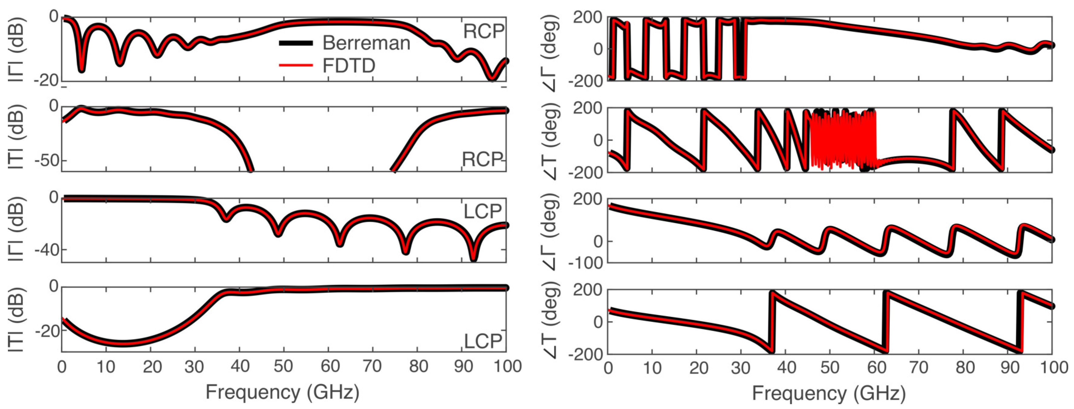
3.1. Propagation in Magnetized Plasma

We first study wave propagation in anisotropic magnetized plasma in which the direction of propagation is along the z-axis and the external DC magnetic field is H = H D C z as in [22] (chap. 8). In this case, the nonzero elements of the permittivity tensor, assuming the e j ω t time convention, are given by
ε x x ( ω ) = ε y y ( ω ) = 1 1 j v ω ω p 2 ω 2 1 j v ω 2 ω b 2 ω 2
ε x y ( ω ) = ε y x ( ω ) = j ω b ω ω p 2 ω 2 1 j v ω 2 ω b 2 ω 2
ε z z ( ω ) = 1 ω p 2 ω 2 1 j v ω
where ω p is the plasma frequency, v is the electron collision rate and ω b is the cyclotron frequency. In view of the tensor elements of Equation (16), the parameters of the CCPR model are derived through the simple algebraic manipulations shown in Table 2.
We study the wave propagation of a Gaussian pulse normally incident to a magnetized plasma slab of 9 mm in thickness, assuming that the static biasing magnetic is parallel to the direction of propagation. The plasma parameters are ω p = 2 π × 50 × 10 9 rad/s, ω b = 3 × 10 11 rad/s, and v c = 2 × 10 10 Hz. The FDTD cell size is Δ z = 75 µm and the time step is chosen as Δ t = Q Δ z / c 0 , where Q = 0.3 is the Courant number and c 0 is the velocity of light in free space. The Gaussian pulse is excited from the left side of the computational domain at the x component of the electric field. The domain is truncated by a 12 cell convolution perfectly matched layer (CPML) [23]. We calculate the reflection ( Γ ) and transmission (T) coefficients for right circularly polarized (RCP) and left circularized polarized (LCP), defined as
T RCP ( ω ) = E x t ( ω ) E x i ( ω ) + j E y t ( ω ) E x i ( ω ) , Γ RCP ( ω ) = E x r ( ω ) E x i ( ω ) + j E y r ( ω ) E x i ( ω )
T LCP ( ω ) = E x t ( ω ) E x i ( ω ) j E y t ( ω ) E x i ( ω ) , Γ LCP ( ω ) = E x r ( ω ) E x i ( ω ) j E y r ( ω ) E x i ( ω )
where E x t and E y t are the x and y components of the transmitted electric field in the frequency domain, respectively, and E x r and E y r are likewise the reflected components. E x i is the x component of the incident wave in the frequency domain. In Figure 1, we validate the proposed FDTD method using as a reference the semi-analytical solution calculated by the Berreman 4 × 4 method [24]. Excellent agreement is observed in a very broad spectral range (0–100 GHz).

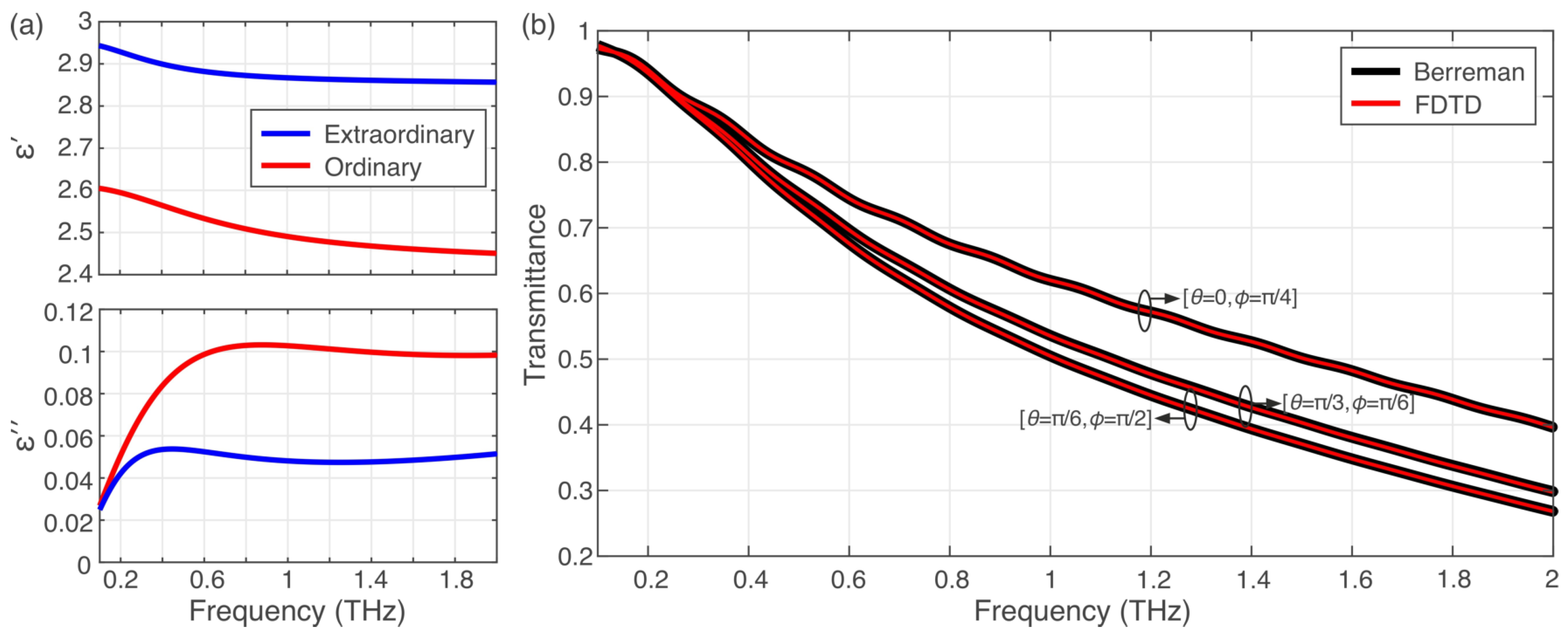
3.2. Terahertz Wave Propagation through a Nematic Liquid Crystal Cell

For NLC materials, the relative permittivity tensor is given by
ε ¯ ¯ ( ω ) = ε o + Δ ε cos 2 θ cos 2 ϕ Δ ε cos 2 θ sin ϕ cos ϕ Δ ε sin θ cos θ cos ϕ Δ ε cos 2 θ sin ϕ cos ϕ ε o + Δ ε cos 2 θ sin 2 ϕ Δ ε sin θ cos θ sin ϕ Δ ε sin θ cos θ cos ϕ Δ ε sin θ cos θ sin ϕ ε o + Δ ε sin 2 θ ,
where θ and ϕ are the tilt and twist angles of the spatially varying LC molecular orientation, respectively, and ε o and ε e are the frequency-dependent ordinary and extraordinary dielectric permittivities, with Δ ε = ε e ε o . The tilt angle is defined as the angle between the nematic director, a unit vector parallel to the NLC optical axis, and the xy plane, whereas the twist angle is measured between the x axis and the projection of the director on the xy plane. The ordinary and extraordinary dielectric permittivities are described as the sum of CCPR terms according to Equation (4).
We demonstrate the efficiency of the proposed FDTD formulation for the case of THz wave propagation through an LC cell. The NLC material is 5CB, whose material dispersion has been described via the modified Lorentz model [25], and the equivalent CCPR parameters are obtained using Table 1. The real and imaginary parts of the extraordinary and ordinary relative permittivity ( ε o , e = ε j ε ) in the considered spectral range are shown in Figure 2a. A layer of 0.5 mm is embedded in a substrate material with a refractive index of 1.5 .
An x polarized plane wave impinges on the slab, and the transmittance after the slab is calculated. The FDTD cell size is chosen to be equal to 0.5 µm, and the computational domain is terminated by a 12-cell CPML. The FDTD time step is set to Δ t = 0.3 Δ z / c 0 and the simulation is run for 60,000 time steps. A direct comparison of the transmittance of the structure obtained by the proposed FDTD scheme and the reference matrix technique is provided in Figure 2b for indicative values of the θ and ϕ angles. Excellent agreement is observed.

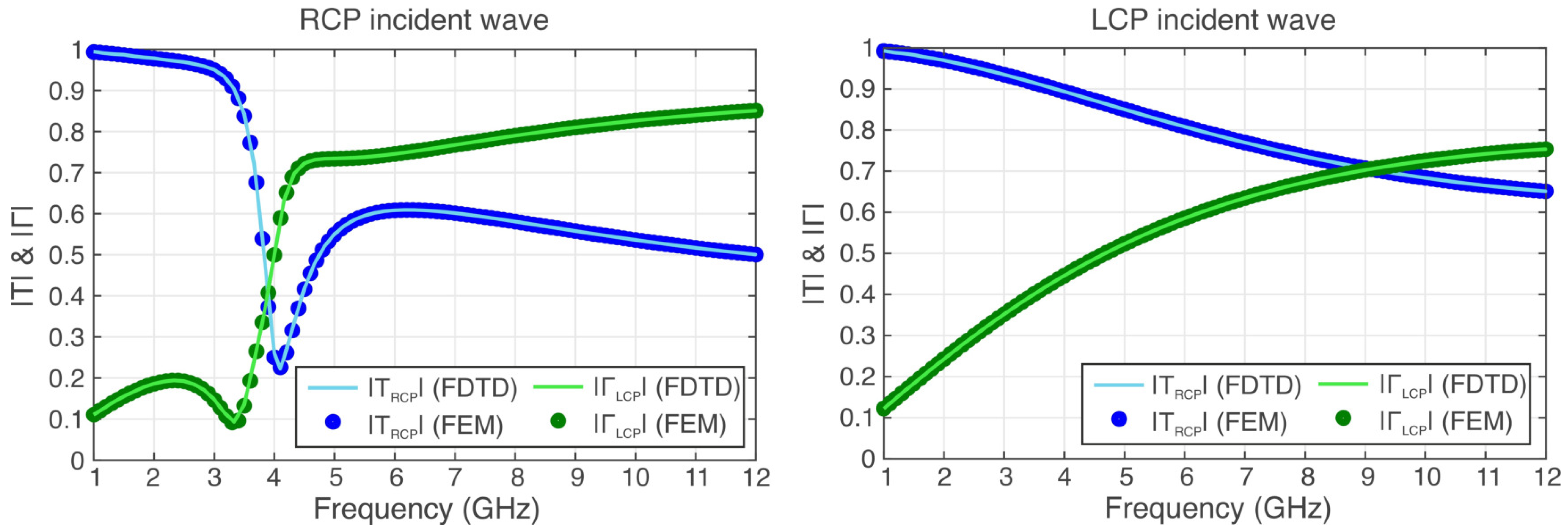
3.3. Propagation in Ferrites

As a last example, we investigate the case of wave propagation through a ferrite slab. The nonzero elements of the permeability tensor are given by [22]
μ x x ( ω ) = μ y y ( ω ) = μ ( ω )
μ y x ( ω ) = μ x y ( ω ) = j κ ( ω )
μ z z ( ω ) = 1
with
μ ( ω ) = 1 + ( ω 0 + j ω a ) ω M ( ω 0 + j ω a ) 2 ω 2
κ ( ω ) = ( ω 0 + j ω a ) ω M ( ω 0 + j ω a ) 2 ω 2 ,
where it is assumed that the magnetic bias is in the z-direction. Loss is accounted for via the complex resonant frequency; namely, ω 0 ω 0 + j ω a . The CCPR parameters for this case are given in Table 3 and they are described by modified Lorentz relations.
A computational domain with 5000 cells with a cell size of 15 µm is assumed, which is backed with a 12-cell CPML. A ferrite slab of thickness 15 mm is surrounded by air, and an amplitude-modulated Gaussian pulse with a frequency range from 500 MHz to 14 GHz is excited and impinges upon the slab. The gyromagnetic response frequency is ω 0 = 2 π × 4 × 10 9 rad/s, while the saturation magnetization frequency is ω M = 2 π × 5.6 × 10 9 rad/s with a = 0.05 and ε r = 10 [26]. The transmission and reflection coefficients for RCP and LCP waves are calculated using the proposed formulation and compared to the finite element method (FEM) solution implemented in the software COMSOL Multiphysics. A direct comparison of the results is provided in Figure 3, once again demonstrating the efficiency of the proposed FDTD algorithm.

4. Conclusions

An FDTD formulation is introduced for the study of anisotropic media with generalized dispersive properties, described by the CCPR function. Both electric and magnetic anisotropy are considered with independently dispersive elements of the electric permittivity and magnetic permeability tensors, respectively. The validity of the proposed algorithm is demonstrated in three case examples involving magnetized plasma, liquid crystals and ferrites by comparing the FDTD results with those obtained with benchmark semi-analytic or numerical solutions.

Author Contributions

Conceptualization, K.P.P. and D.C.Z.; methodology, K.P.P.; software, K.P.P.; validation, K.P.P. and D.C.Z.; writing—original draft preparation, K.P.P.; writing—review and editing, D.C.Z.; supervision, D.C.Z. All authors have read and agreed to the published version of the manuscript.

Funding

This research received no external funding.

Institutional Review Board Statement

Not applicable.

Informed Consent Statement

Not applicable.

Data Availability Statement

The data that support the findings of this study are available from the authors upon reasonable request.

Conflicts of Interest

The authors declare no conflict of interest.

References

  1. Inan, U.; Marshall, R. Numerical Electromagnetics: The FDTD Method; Cambridge University Press: Cambridge, UK, 2011. [Google Scholar]
  2. Young, J.L.; Nelson, R.O. A summary and systematic analysis of FDTD algorithms for linearly dispersive media. IEEE Antennas Propag. Mag. 2001, 43, 61–126. [Google Scholar] [CrossRef]
  3. Hunsberger, F.; Luebbers, R.; Kunz, K. Finite-difference time-domain analysis of gyrotropic media. I. Magnetized plasma. IEEE Trans. Antennas Propag. 1992, 40, 1489–1495. [Google Scholar] [CrossRef]
  4. Huang, S.J.; Li, F. FDTD Simulation of Electromagnetic Propagation in Magnetized Plasma Using Z Transforms. Int. J. Infrared Millim. Waves 2004, 25, 815–825. [Google Scholar] [CrossRef]
  5. Mosallaei, H. FDTD-PLRC technique for modeling of anisotropic-dispersive media and metamaterial devices. IEEE Trans. Electromagn. Compat. 2007, 49, 649–660. [Google Scholar] [CrossRef]
  6. Nayyeri, V.; Soleimani, M.; Rashed Mohassel, J.; Dehmollaian, M. FDTD Modeling of Dispersive Bianisotropic Media Using Z-Transform Method. IEEE Trans. Antennas Propag. 2011, 59, 2268–2279. [Google Scholar] [CrossRef]
  7. Al-Jabr, A.A.; Alsunaidi, M.A.; Khee, T.; Ooi, B.S. A Simple FDTD Algorithm for Simulating EM-Wave Propagation in General Dispersive Anisotropic Material. IEEE Trans. Antennas Propag. 2013, 61, 1321–1326. [Google Scholar] [CrossRef] [Green Version]
  8. Zografopoulos, D.C.; Prokopidis, K.P.; Dąbrowski, R.; Beccherelli, R. Time-domain modeling of dispersive and lossy liquid-crystals for terahertz applications. Opt. Mater. Express 2014, 4, 449. [Google Scholar] [CrossRef]
  9. Xi, X.; Li, Z.; Liu, J.; Zhang, J. FDTD Simulation for Wave Propagation in Anisotropic Dispersive Material Based on Bilinear Transform. IEEE Trans. Antennas Propag. 2015, 63, 5134–5138. [Google Scholar] [CrossRef]
  10. Han, M.; Dutton, R.; Fan, S. Model dispersive media in finite-difference time-domain method with complex-conjugate pole-residue pairs. IEEE Microw. Wirel. Compon. Lett. 2006, 16, 119–121. [Google Scholar]
  11. Michalski, K. On the Low-Order Partial-Fraction Fitting of Dielectric Functions at Optical Wavelengths. IEEE Trans. Antennas Propag. 2013, 61, 6128–6135. [Google Scholar] [CrossRef]
  12. Choi, H.; Baek, J.-W.; Jung, K.-Y. Numerical Stability and Accuracy of CCPR-FDTD for Dispersive Media. IEEE Trans. Antennas Propag. 2020, 68, 7717–7720. [Google Scholar] [CrossRef]
  13. Prokopidis, K.P.; Zografopoulos, D.C. Time-domain numerical scheme based on low-order partial-fraction models for the broadband study of frequency-dispersive liquid crystals. J. Opt. Soc. Am. B 2016, 33, 622–629. [Google Scholar] [CrossRef]
  14. Prokopidis, K.P.; Zografopoulos, D.C. One-Step Leapfrog ADI-FDTD Method Using the Complex-Conjugate Pole-Residue Pairs Dispersion Model. IEEE Microw. Wirel. Compon. Lett. 2018, 28, 1068–1070. [Google Scholar] [CrossRef]
  15. Prokopidis, K.P.; Zografopoulos, D.C. A Unified FDTD/PML Scheme Based on Critical Points for Accurate Studies of Plasmonic Structures. J. Light. Technol. 2013, 31, 2467–2476. [Google Scholar] [CrossRef]
  16. Prokopidis, K.P.; Zografopoulos, D.C. Investigation of the Stability of ADE-FDTD Methods for Modified Lorentz Media. IEEE Microw. Wirel. Compon. Lett. 2014, 24, 659–661. [Google Scholar] [CrossRef]
  17. Rekanos, I.T.; Papadopoulos, T.G. FDTD Modeling of Wave Propagation in Cole–Cole Media With Multiple Relaxation Times. IEEE Antennas Wirel. Propag. Lett. 2010, 9, 67–69. [Google Scholar] [CrossRef]
  18. Rekanos, I.T. FDTD Modeling of Havriliak-Negami Media. IEEE Microw. Wireless Compon. Lett. 2012, 92, 49–51. [Google Scholar] [CrossRef]
  19. Gustavsen, B.; Semlyen, A. Rational approximation of frequency domain responses by vector fitting. IEEE Trans. Power Deliv. 1999, 14, 1052–1061. [Google Scholar] [CrossRef] [Green Version]
  20. Liu, D.; Michalski, K.A. Comparative study of bio-inspired optimization algorithms and their application to dielectric function fitting. J. Electromagn. Waves Appl. 2012, 30, 1885–1894. [Google Scholar] [CrossRef]
  21. Garcia-Vergara, M.; Demésy, G.; Zolla, F. Extracting an accurate model for permittivity from experimental data: Hunting complex poles from the real line. Opt. Lett. 2017, 42, 1145–1148. [Google Scholar] [CrossRef] [Green Version]
  22. Ishimaru, A. Electromagnetic Wave Propagation, Radiation, and Scattering: From Fundamentals to Applications; IEEE Press Series on Electromagnetic Wave Theory; John Wiley & Sons, Inc.: Hoboken, NJ, USA, 2017. [Google Scholar]
  23. Roden, J.A.; Gedney, S.D. Convolution PML (CPML): An efficient FDTD implementation of the CFS-PML for arbitrary media. Microw. Opt. Technol. Lett. 2000, 27, 334–339. [Google Scholar] [CrossRef]
  24. Stallinga, S. Berreman 4 × 4 matrix method for reflective liquid crystal displays. J. Appl. Phys. 1999, 85, 3023–3031. [Google Scholar] [CrossRef]
  25. Zografopoulos, D.C.; Prokopidis, K.P.; Tofani, S.; Chojnowska, O.; Dąbrowski, R.; Kriezis, E.E.; Beccherelli, R. An ADE-FDTD Formulation for the Study of Liquid-Crystal Components in the Terahertz Spectrum. Mol. Cryst. Liq. Cryst. 2015, 619, 49–60. [Google Scholar] [CrossRef]
  26. Prosvirnin, S.L.; Dmitriev, V.A. Electromagnetic wave diffraction by array of complex-shaped metal elements placed on ferromagnetic substrate. Eur. Phys. J. Appl. Phys. 2010, 49, 33005. [Google Scholar] [CrossRef]
Figure 1. The magnitude and phase of the transmission/reflection coefficients for RCP/LCP waves propagating through magnetized plasma calculated by the proposed FDTD method and the Berreman 4 × 4 matrix method.
Applsci 11 03844 g001
Figure 2. (a) The ordinary and extraordinary relative permittivities of 5CB in the low THz spectrum. (b) Transmittance calculated by the proposed FDTD method and the Berreman method.
Applsci 11 03844 g002
Figure 3. The reflection and transmission coefficients for the RCP and LCP polarizations.
Applsci 11 03844 g003
Table 1. CCPR parameters for the description of various known dispersion models.
ModelExpressionParameters of the CCPR Model: σ , ( c p , a p )
Drude ω p 2 j ω ( j ω + ν ) ε 0 ω p 2 / ν , ( 0.5 ω p 2 / ν , ν )
Debye Δ ε 1 + j ω τ 0, ( 0.5 Δ ε / τ , 1 / τ )
Lorentz Δ ε ω p 2 ω p 2 + j ω δ + ( j ω ) 2 0, j Δ ε ω p 2 2 ω p 2 δ 2 , δ j ω p 2 δ 2
Critical Points A p Ω p e j ϕ p Ω p + ω j Γ p
+ e j ϕ p Ω p ω + j Γ p
0, A p Ω p ( sin ϕ p j cos ϕ p ) , Γ p Ω p j
Sellmeier B λ 2 λ 2 C , λ = ω 2 π c 0, 1 2 j B 2 π c C , j 2 π c C
Modified Lorentz a 0 + j a 1 ω b 0 + j ω b 1 + ( j ω ) 2 0, ( c p = a 0 + a p a 1 a p a p * , a p = 1 2 b 1 + j 4 b 0 b 1 2 ) or
0, ( c p 1 = a 0 + a p 1 a 1 a p 1 a p 2 , a p 1 = 0.5 b 1 + b 1 2 4 b 0 ,
c p 2 = a 1 c p 1 , a p 2 = 0.5 b 1 + b 1 2 4 b 0 )
Table 2. CCPR parameters for magnetized plasma.
Tensor ElementParameters: σ , ( c p , a p )
ε x x ε 0 ω p 2 v v 2 + ω b 2 , 0.5 ω p 2 v + j ω b v 2 + ω b 2 , v + j ω b
ε x y ε 0 ω p 2 ω b v 2 + ω b 2 , 0.5 ω p 2 ω b + j v v 2 + ω b 2 , v + j ω b
ε z z ε 0 ω p 2 / v , ( 0.5 ω p 2 / v 2 , v )
Table 3. CCPR parameters for lossy ferrites.
Tensor’s ElementParameters: σ , ( c p , a p )
μ x x , μ y y 0 , ( 0.5 j ω M , j ω 0 )
μ x y 0 , ( 0.5 ω M , j ω 0 )
μ y x 0 , ( 0.5 ω M , j ω 0 )
Publisher’s Note: MDPI stays neutral with regard to jurisdictional claims in published maps and institutional affiliations.

