
Different Causal Factors Occur between Land Use/Cover and Vegetation Classification Systems but Not between Vegetation Classification Levels in the Highly Disturbed Jing-Jin-Ji Region of China

 ,
, 
Abstract
1. Introduction
2. Data and Method
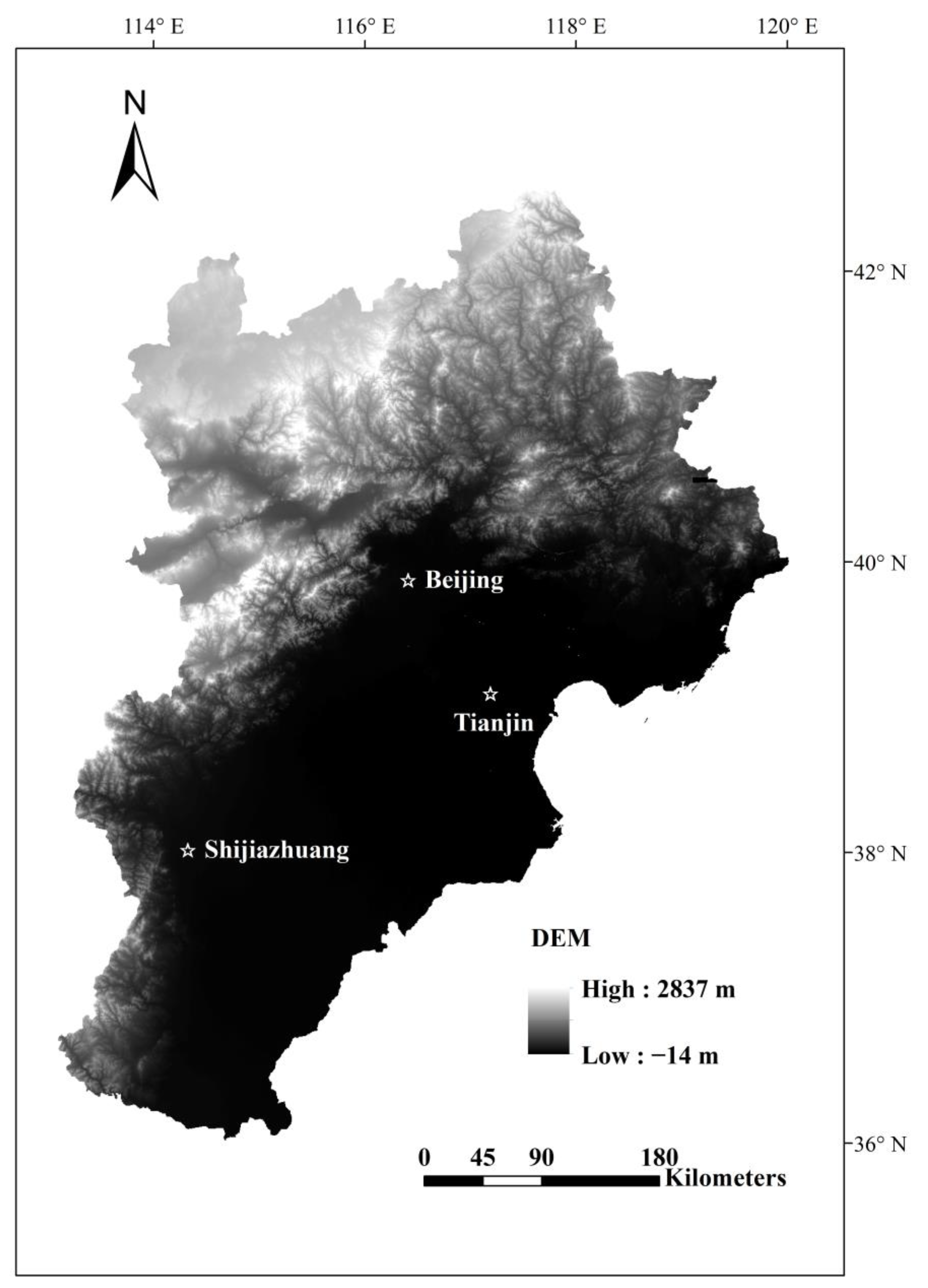
2.1. Study Area
2.2. Land Use/Cover and Vegetation Category Data and Landscape Metrics
2.3. Geographic, Soil, Precipitation, Temperature, Atmospheric, and Anthropogenic Disturbance Data
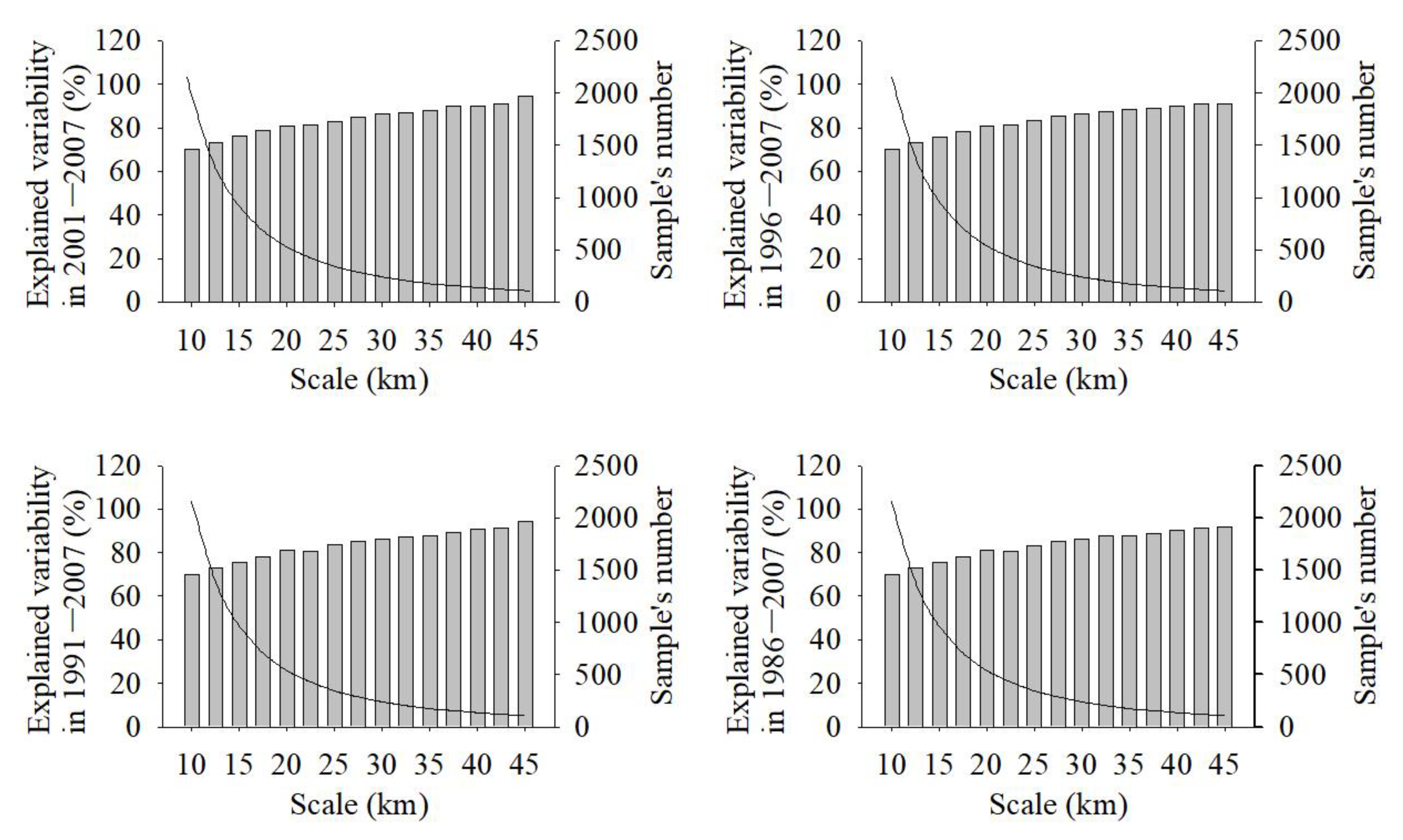
2.4. Suitable Spatial Scale and Redundancy Analysis in Four Periods
3. Results
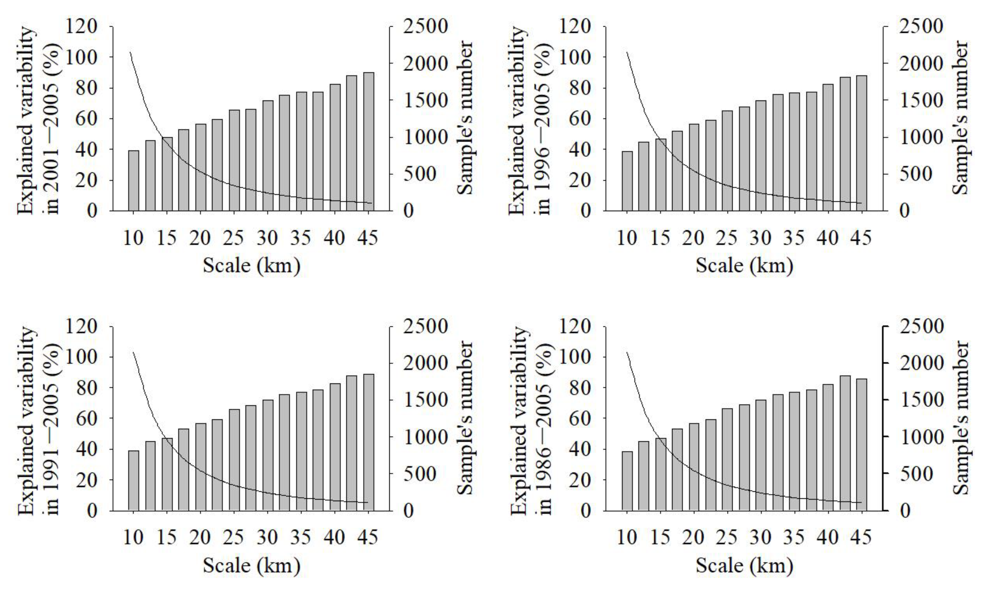
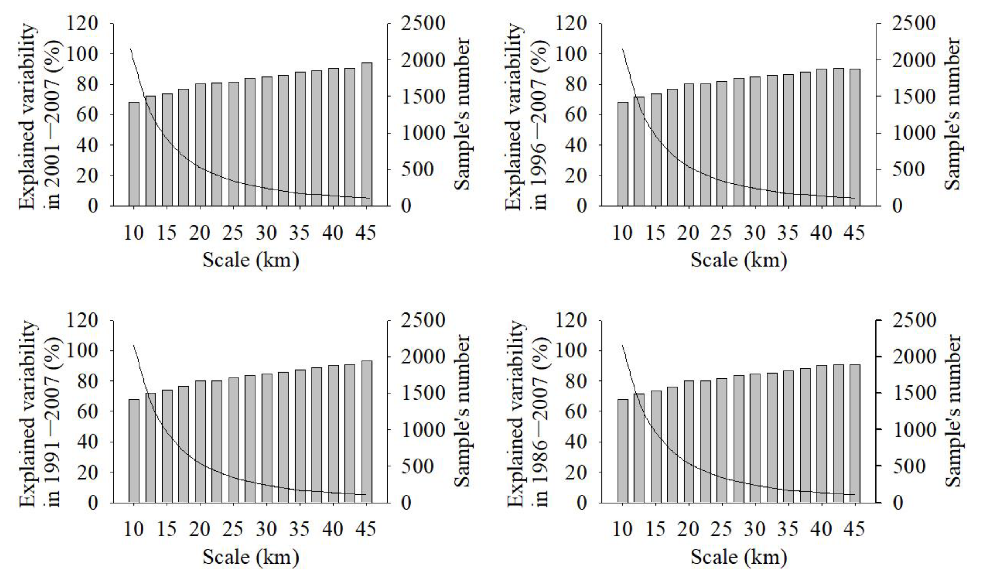
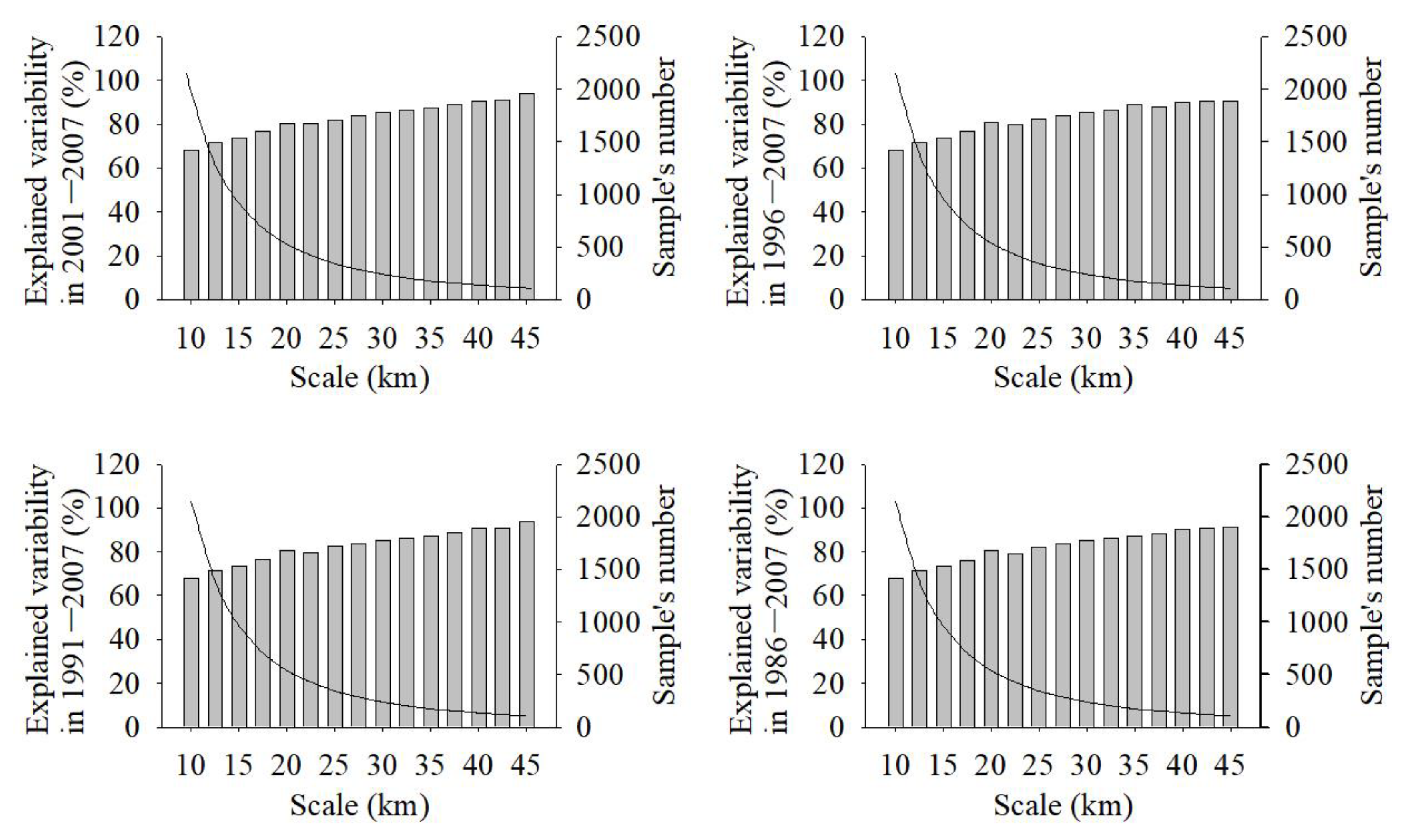
3.1. Suitable Spatial Scale
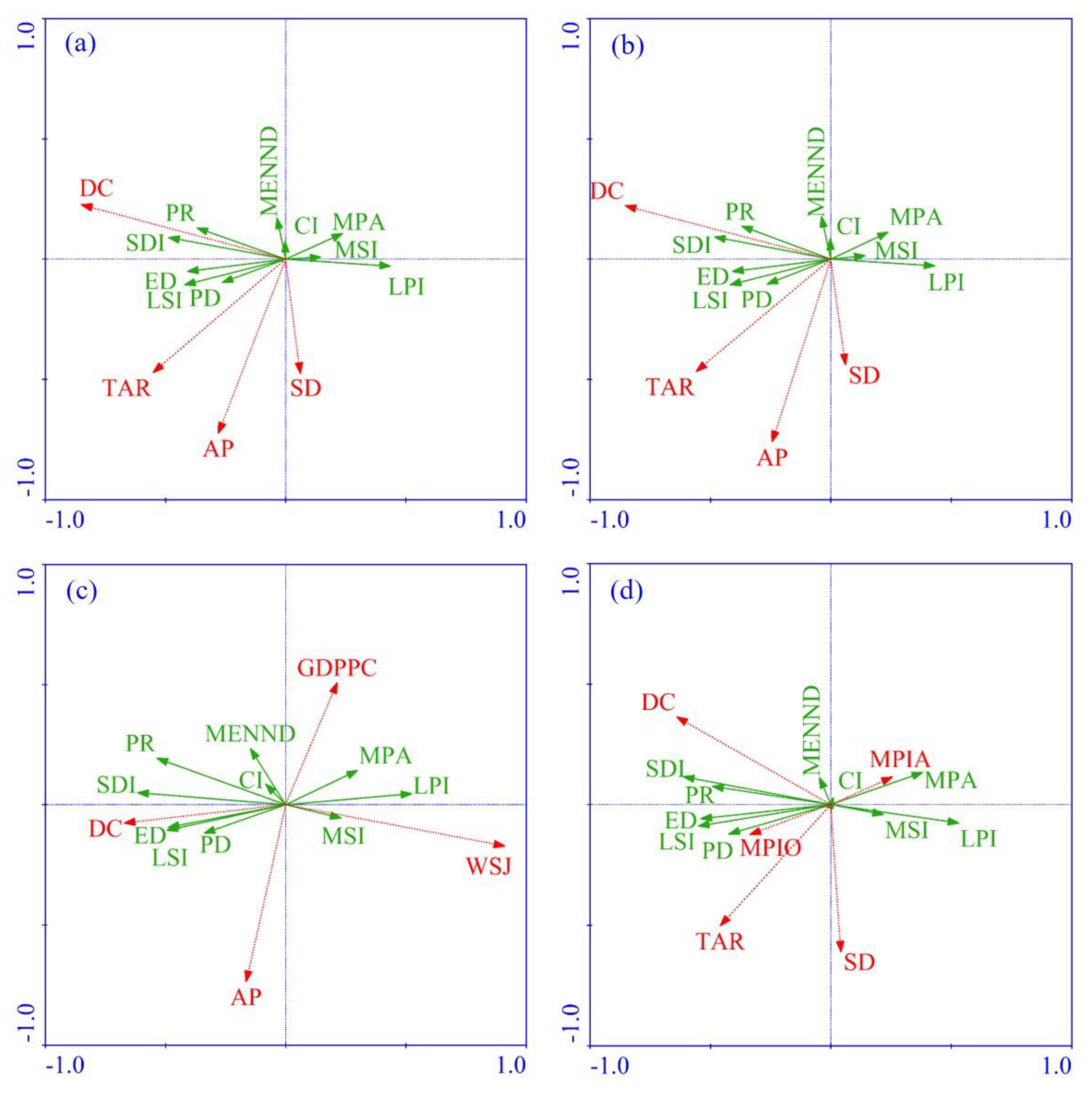
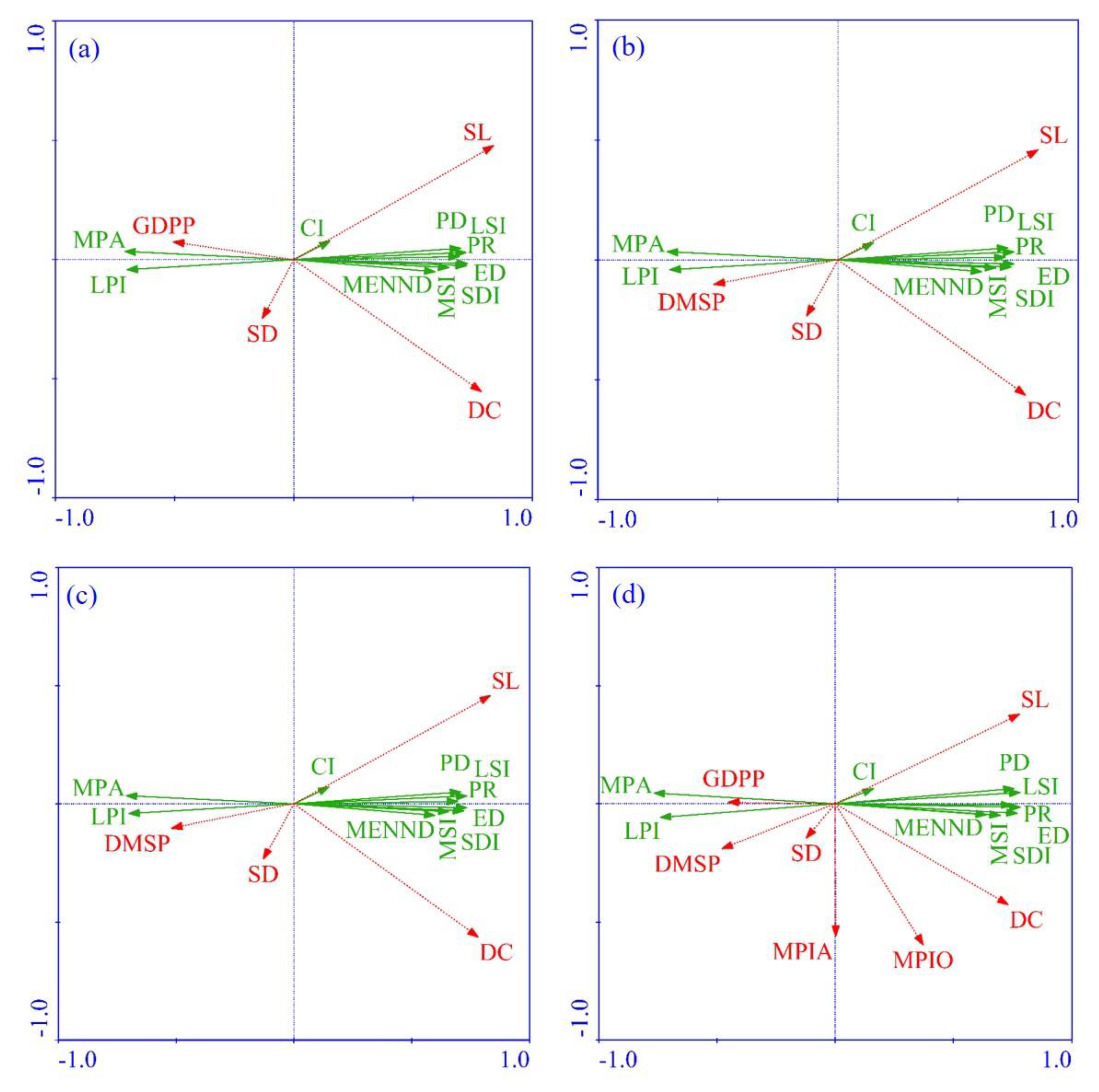
3.2. Causal Factors for Land Use/Cover Patterns and Correlations between Landscape Metrics and Environmental Factors
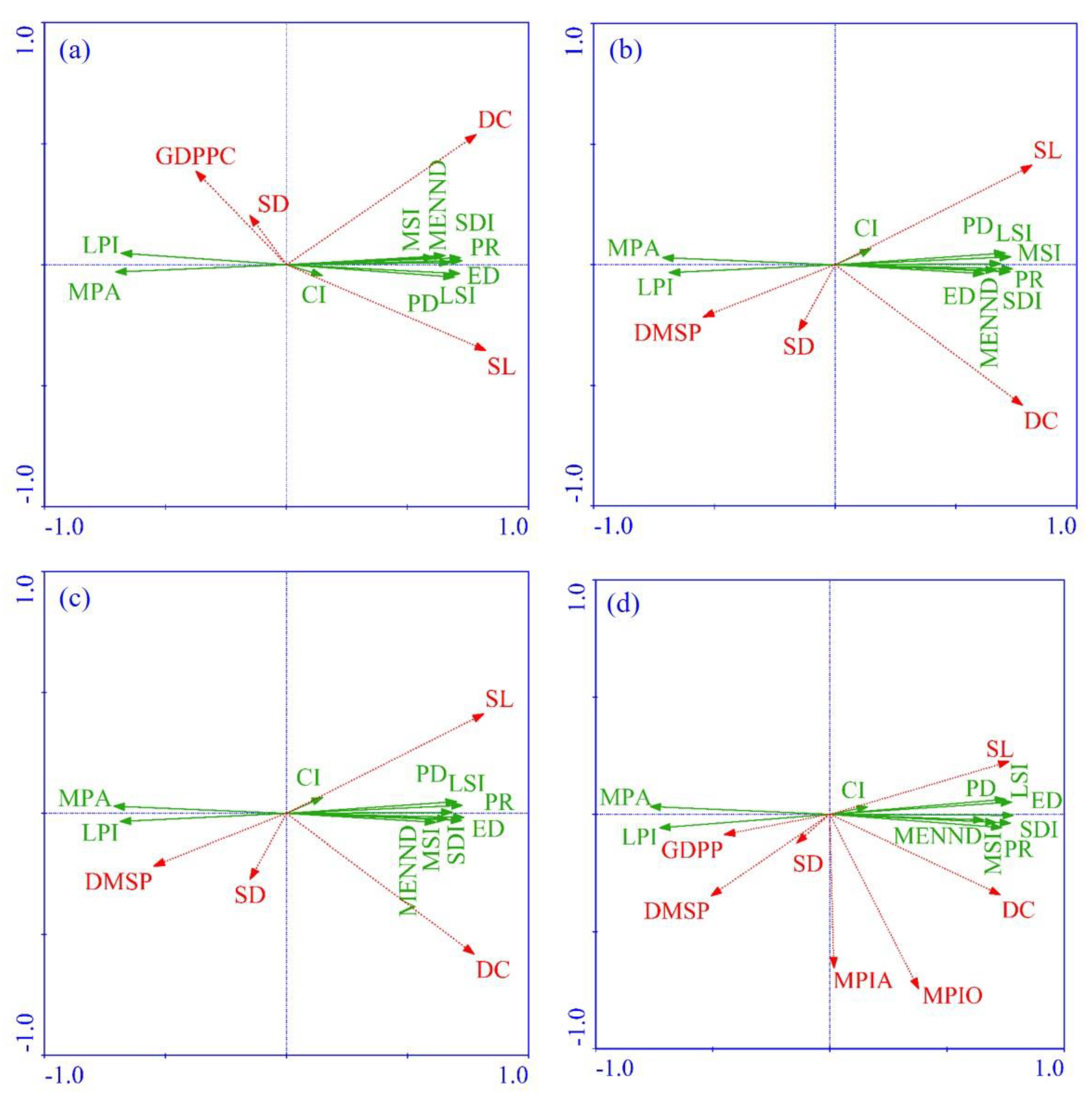
3.3. Causal Factors for Vegetation Group Patterns and Correlations between Landscape Metrics and Environmental Factors
3.4. Causal Factors for Vegetation Type Patterns and Correlations between Landscape Metrics and Environmental Factors
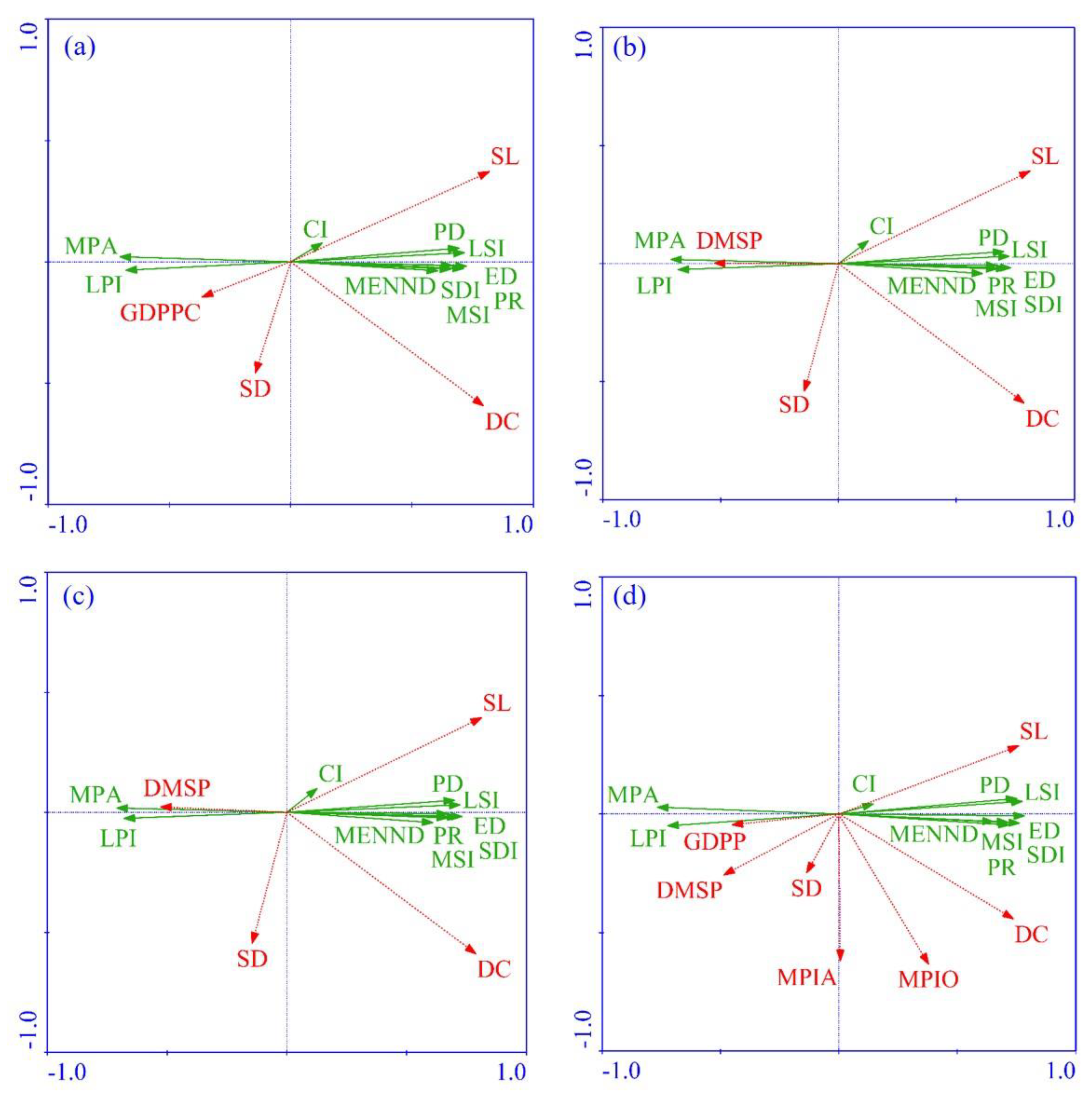
3.5. Causal Factors for Formation and Subformation Patterns and Correlations between Landscape Metrics and Environmental Factors
4. Discussion
4.1. Factors Affecting Landscape Patterns in Different Classification
4.2. Different Classification
4.3. Other Possible Factors Not Considered in This Research
5. Conclusions
Author Contributions
Funding
Institutional Review Board Statement
Informed Consent Statement
Data Availability Statement
Acknowledgments
Conflicts of Interest
Appendix A

| Land Use/Cover | Vegetation Groups | Vegetation Types | Formations and Subformations |
|---|---|---|---|
| 1. Woodland | 1. Needleleaf forest | 1. Cold-temperate and temperate mountains needleleaf forest | 1. Larix principis-rupprechtii forest |
| 2. Temperate needleleaf forest | 2. Pinus tabulaeformis forest | ||
| 3. Platycladus orientalis forest | |||
| 2. Broadleaf forest | 3. Temperate broadleaf deciduous forest | 4. Quercus mongolica forest | |
| 5. Quercus liaotungensis forest | |||
| 6. Quercus aliena forest | |||
| 7. Quercus acutissima forest | |||
| 8. Quercus variabilis forest | |||
| 9. Robinia pseudoacacia forest | |||
| 10. Salix matsudana forest | |||
| 11. Populus simonii forest | |||
| 12. Populus nigra forest | |||
| 13. Populus davidiana forest | |||
| 14. Chosenia arbutifolis, Populus suaveolens forest | |||
| 15. Betula platyphylla forest | |||
| 4. Temperate microphyllous deciduous woodland | 16. Ulmus macrocarpa woodland | ||
| 3. Scrub | 5.Temperate broadleaf deciduous scrub | 17. Corylus heterophylla scrub | |
| 18. Lespedeza bicolor scrub | |||
| 19. Prunus armeniaca var. ansa scrub | |||
| 20. Gleditsia heterophylla scrub | |||
| 21. Vitex negundo var. heterophylla, Zizyphus jujuba var. spinosa scrub | |||
| 22. Cotinus coggygria var. cinerea scrub | |||
| 23. Spiraea spp. scrub | |||
| 24. Ostryopsis davidiana scrub | |||
| 25. Hippophae rhamnoides scrub | |||
| 26. Rosa spp., Cotoneaster spp. scrub | |||
| 27. Tamarix chinensis scrub | |||
| 2. The grass | 4. Steppe | 6. Temperate grass-forb meadow steppe | 28. Festuca ovina, forb meadow steppe |
| 29. Stipa baicalensis, forb meadow steppe | |||
| 30. Bothriochloa ischaemum, forb meadow steppe | |||
| 31. Filifolium sibiricum, grass-forb meadow steppe | |||
| 7. Temperate needlegrass arid steppe | 32. Aneurolepidium chinense, needlegrass steppe | ||
| 33. Stipa grandis steppe | |||
| 34. Stipa krylovii steppe | |||
| 35. Stipa bungiana steppe | |||
| 36. Koeleria cristata, Agropyron cristatum, dwarf needlegrass steppe | |||
| 37. Thymus mongolicus, needlegrass steppe | |||
| 38. Artemisia frigida, dwarf needlegrass steppe | |||
| 39. Artemisia gmelinii, grass steppe | |||
| 40. Artemisia giraldii, grass steppe | |||
| 5. Grass-forb community | 8. Temperate grass-forb community | 41. Bothriochloa ischaemum community | |
| 42. Themeda triandra var. japonica community | |||
| 6. Meadow | 9. Temperate grass and forb meadow | 43. Arundinella hirta, Spodiopogon sibiricus, forb meadow | |
| 44. Imperata cylindrica var. major meadow | |||
| 45. Carex spp., forb meadow | |||
| 46. Contain Carex spp. | |||
| 10. Temperate grass, Carex and forb swamp meadow | 47. Agrostis alba, Hordeum bogdanii swamp meadow | ||
| 11. Temperate grass and forb holophytic meadow | 48. Phragmites communis holophytic meadow | ||
| 49. Achnatherum splendens holophytic meadow | |||
| 50. Kalidinm spp., Puccinellia distans holophytic meadow | |||
| 51. Suaeda glauca holophytic meadow | |||
| 3. Water area | 7. Swamp | 12. Cold-temperate and temperate swamp | 52. Phragmites communis swamp |
| 4. Cultivated land | 8. Cultural vegetation | 13. One crop annually and cold-resistant economic crops | 53. Spring wheat, middle and late crop soybean, corn, Chinese sorghum; sugar beet, sunflower, flux; apple (the seedling takes cover in winter) |
| 54. Spring wheat, naked oats, buckwheat, potatoes; flux | |||
| 14. One crop annually, cold-resistant economic crops and deciduous orchards | 55. Spring (winter) wheat, Chinese sorghum, millet, gruel, Medicago sativa; sunflower, sugar beet; apple, pear, date, valnut | ||
| 15. Three crops two years and two crops annually non irrigation, deciduous orchards | 56. Winter wheat, corn, Chinese sorghum, millet, sweet potatoes; peanut; apple, pear, hawthorn, persimmon, walnut, chestnut, date, grape (takes cover in winter) | ||
| 57. Winter wheat, corn, Chinese sorghum, sweet potatoes; cotton, tobacco, peanut, sesame; apple, pear, hauthorn, persimmon, walnut, pomegranate, grape | |||
| 5. The land of industry, mining and residence in urban and rural | 9. No vegetation | 16. No vegetation | 58. No vegetation |
| 6. Unused land |
| Categories of Variable | Variables |
|---|---|
| Geography | Elevation |
| Aspect | |
| Slope | |
| Soil | Texture class |
| Available water storage capacity | |
| Drainage class | |
| Soil depth | |
| Subsoil base saturation | |
| Subsoil Calcium Carbonate | |
| Subsoil Gypsum | |
| The cation exchange capacity in subsoil | |
| Percentage clay in the subsoil | |
| The electrical conductivity of subsoil | |
| The exchangeable sodium percentage in subsoil | |
| Volume percentage gravel in the subsoil | |
| The percentage of organic carbon in subsoil | |
| pH in the subsoil | |
| Bulk density of subsoil | |
| Percentage sand in the subsoil | |
| Percentage silt in the subsoil | |
| Topsoil base saturation | |
| Topsoil Calcium Carbonate | |
| Topsoil Gypsum | |
| The cation exchange capacity in topsoil | |
| Percentage clay in the topsoil | |
| The electrical conductivity of topsoil | |
| The exchangeable sodium percentage in topsoil | |
| Volume percentage gravel in the topsoil | |
| The percentage of organic carbon in topsoil | |
| pH in the topsoil | |
| Bulk density of topsoil | |
| Percentage sand in the topsoil | |
| Percentage silt in the topsoil | |
| Precipitation | Annual precipitation |
| Monthly precipitation in April and October | |
| Precipitation of wettest month (i.e., Monthly precipitation in July) | |
| Precipitation of driest month (i.e., Monthly precipitation in January) | |
| Precipitation of warmest quarter | |
| Precipitation of coldest quarter | |
| Temperature | Minimum temperature in April, July, and October |
| Maximum temperature in January, April, and October | |
| Monthly average temperature in January, April, July, and October | |
| Max temperature of warmest month (i.e., Maximum temperature in July) | |
| Min temperature of coldest month (i.e., Minimum temperature in January) | |
| Mean annual temperature | |
| Mean diurnal range | |
| Isothermality | |
| Temperature annual range | |
| Mean temperature of warmest quarter | |
| Mean temperature of coldest quarter | |
| Atmospherics | Water vapor pressure in January, April, July, and October |
| Wind speed in January, April, July, and October | |
| Anthropogenic disturbance | Population |
| Gross domestic product | |
| Gross domestic product from primary industry | |
| Gross domestic product from secondary industry | |
| Gross domestic product from tertiary industry | |
| Gross domestic product per capita | |
| Gross domestic product per unit area | |
| Defense meteorological satellite program/operational linescan system night light |


References
- Editorial Committee of Vegetation Map of China, the Chinese Academy of Science. The Vegetation Map of the People’s Republic of China (1:1 000 000); Geological Publishing House: Beijing, China, 2007; pp. 1–66. [Google Scholar]
- Gao, N.; Zhou, J.; Zhang, X.; Cai, W.; Guan, T.; Jiang, L.; Du, H.; Yang, D.; Cong, Z.; Zheng, Y. Correlation between vegetation and environment at different levels in an arid, mountainous region of China. Ecol. Evol. 2017, 7, 5482–5492. [Google Scholar] [CrossRef]
- Braimoh, A.K. Random and systematic land-cover transitions in northern Ghana. Agr. Ecosyst. Environ. 2006, 113, 254–263. [Google Scholar] [CrossRef]
- Geri, F.; Rocchini, D.; Chiarucci, A. Landscape metrics and topographical determinants of large-scale forest dynamics in a Mediterranean landscape. Landsc. Urban Plan. 2010, 95, 46–53. [Google Scholar] [CrossRef]
- Sivakumar, M.V.K. Interactions between climate and desertification. Agr. For. Meteorol. 2007, 142, 143–155. [Google Scholar] [CrossRef]
- Vitousek, P.M.; Mooney, H.A.; Lubchenco, J.; Melillo, J.M. Human domination of Earth’s ecosystems. Science 1997, 277, 494–499. [Google Scholar] [CrossRef]
- Petit, C.C.; Lambin, E.F. Impact of data integration technique on historical land-use/land-cover change: Comparing historical maps with remote sensing data in the Belgian Ardennes. Landsc. Ecol. 2002, 17, 117–132. [Google Scholar] [CrossRef]
- Motzkin, G.; Wilson, P.; Foster, D.R.; Allen, A. Vegetation patterns in heterogeneous landscapes: The importance of history and environment. J. Veg. Sci. 1999, 10, 903–920. [Google Scholar] [CrossRef]
- Huete, A. Vegetation’s responses to climate variability. Nature 2016, 531, 181–182. [Google Scholar] [CrossRef] [PubMed]
- Zhou, J.; Lai, L.; Guan, T.; Cai, W.; Gao, N.; Zhang, X.; Yang, D.; Cong, Z.; Zheng, Y. Comparison modeling for alpine vegetation distribution in an arid area. Environ. Monit. Assess. 2016, 188, 408. [Google Scholar] [CrossRef] [PubMed]
- Liang, T.; Yang, S.; Feng, Q.; Liu, B.K.; Zhang, R.P.; Huang, X.D.; Xie, H.J. Multi-factor modeling of above-ground biomass in alpine grassland: A case study in the Three-River Headwaters Region, China. Remote Sens. Environ. 2016, 186, 164–172. [Google Scholar] [CrossRef]
- Zhu, Z.; Piao, S.; Myneni, R.B.; Huang, M.; Zeng, Z.; Canadell, J.G.; Ciais, P.; Sitch, S.; Friedlingstein, P.; Arneth, A.; et al. Greening of the Earth and its drivers. Nat. Clim. Chang. 2016, 6, 791–795. [Google Scholar] [CrossRef]
- Yang, Y.H.; Fang, J.Y.; Pan, Y.D.; Ji, C.J. Aboveground biomass in Tibetan grasslands. J. Arid Environ. 2009, 73, 91–95. [Google Scholar] [CrossRef]
- Zhang, G.; Biradar, C.M.; Xiao, X.; Dong, J.; Zhou, Y.; Qin, Y.; Zhang, Y.; Liu, F.; Ding, M.; Thomas, R.J. Exacerbated grassland degradation and desertification in Central Asia during 2000–2014. Ecol. Appl. 2018, 28, 442–456. [Google Scholar] [CrossRef] [PubMed]
- Chen, L.; Li, H.; Zhang, P.; Zhao, X.; Zhou, L.; Liu, T.; Hu, H.; Bai, Y.; Shen, H.; Fang, J. Climate and native grassland vegetation as drivers of the community structures of shrub-encroached grasslands in Inner Mongolia, China. Landsc. Ecol. 2015, 30, 1627–1641. [Google Scholar] [CrossRef]
- Chen, X.; An, S.; Inouye, D.W.; Schwartz, M.D. Temperature and snowfall trigger alpine vegetation green-up on the world’s roof. Glob. Chang. Biol. 2015, 21, 3635–3646. [Google Scholar] [CrossRef]
- Zuo, X.; Zhao, X.; Zhao, H.; Zhang, T.; Li, Y.; Wang, S.; Li, W.; Powers, R. Scale dependent effects of environmental factors on vegetation pattern and composition in Horqin Sandy Land, Northern China. Geoderma 2012, 173–174, 1–9. [Google Scholar] [CrossRef]
- Mayaux, P.; Pekel, J.F.; Desclee, B.; Donnay, F.; Lupi, A.; Achard, F.; Clerici, M.; Bodart, C.; Brink, A.; Nasi, R.; et al. State and evolution of the African rainforests between 1990 and 2010. Phil. Trans. R. Soc. B 2013, 368, 20120300. [Google Scholar] [CrossRef]
- Peng, Y.; Mi, K.; Qing, F.; Xue, D. Identification of the main factors determining landscape metrics in semi-arid agro-pastoral ecotone. J. Arid Environ. 2016, 124, 249–256. [Google Scholar] [CrossRef]
- Villers-Ruiz, L.; Trejo-Vazquez, I.; Lopez-Blanco, J. Dry vegetation in relation to the physical environment in the Baja California Peninsula, Mexico. J. Veg. Sci. 2003, 14, 517–524. [Google Scholar] [CrossRef]
- Yang, Y.; Zhu, Q.; Peng, C.; Wang, H.; Xue, W.; Lin, G.; Wen, Z.; Jie, C.; Wang, M.; Liu, G.; et al. A novel approach for modelling vegetation distributions and analysing vegetation sensitivity through trait-climate relationships in China. Sci. Rep. 2016, 6, 24110. [Google Scholar] [CrossRef]
- Borcard, D.; Gillet, F.; Legendre, P. Numerical Ecology with R; Lai, J., Translator; Higher Education Press: Beijing, China, 2014; pp. 104–201. [Google Scholar]
- Leps, J.; Smilauer, P. Multivariate Analysis of Ecological Data Using CANOCO; Cambridge University Press: New York, NY, USA, 2003; pp. 1–73. [Google Scholar]
- Dias, E.; Melo, C. Factors influencing the distribution of Azorean mountain vegetation: Implications for nature conservation. Biodivers. Conserv. 2010, 19, 3311–3326. [Google Scholar] [CrossRef]
- Fanfarillo, E.; Petit, S.; Dessaint, F.; Rosati, L.; Abbate, G. Species composition, richness, and diversity of weed communities of winter arable land in relation to geo-environmental factors: A gradient analysis in mainland Italy. Botany 2020, 98, 381–392. [Google Scholar] [CrossRef]
- Nowak, A.; Nowak, S.; Nobis, M.; Nobis, A. Crop type and altitude are the main drivers of species composition of arable weed vegetation in Tajikistan. Weed Res. 2015, 55, 525–536. [Google Scholar] [CrossRef]
- Zuo, X.; Zhao, X.; Zhao, H.; Zhang, T.; Guo, Y.; Li, Y.; Huang, Y. Spatial heterogeneity of soil properties and vegetation–soil relationships following vegetation restoration of mobile dunes in Horqin Sandy Land, Northern China. Plant Soil 2009, 318, 153–167. [Google Scholar] [CrossRef]
- Schindler, S.; von Wehrden, H.; Poirazidis, K.; Wrbka, T.; Kati, V. Multiscale performance of landscape metrics as indicators of species richness of plants, insects and vertebrates. Ecol. Indic. 2012, 31, 41–48. [Google Scholar] [CrossRef]
- Xie, Y.; Qiu, K.; Xu, D.; Shi, X.; Qi, T.; Richard, P. Spatial heterogeneity of soil and vegetation characteristics and soil-vegetation relationships along an ecotone in Southern Mu Us Sandy Land, China. J. Soils Sediments 2015, 15, 1584–1601. [Google Scholar] [CrossRef]
- Cunningham, R.B.; Lindenmayer, D.B.; Crane, M.; Michael, D.R.; Barton, P.S.; Gibbons, P.; Okada, S.; Ikin, K.; Stein, J.A.R. The law of diminishing returns: Woodland birds respond to native vegetation cover at multiple spatial scales and over time. Divers. Distrib. 2014, 20, 59–71. [Google Scholar] [CrossRef]
- Wu, J.G. Landscape Ecology—Pattern, Process, Scale and Hierarchy; Higher Education Press: Beijing, China, 2000; pp. 95–150. [Google Scholar]
- Zhang, Z.; Van Coillie, F.; De Clercq, E.M.; Ou, X.; De Wulf, R. Mountain vegetation change quantification using surface landscape metrics in Lancang watershed, China. Ecol. Indic. 2013, 31, 49–58. [Google Scholar] [CrossRef]
- Wang, L.; Gong, B.L. Collaborative Governance of Ecological Space in Beijing-Tianjin-Hebei Region. J. Tianjin Adm. Inst. 2018, 20, 38–44. (In Chinese) [Google Scholar]
- Jin, J.; Sheppard, S.R.J.; Jia, B.; Wang, C. Planning to Practice: Impacts of Large-Scale and Rapid Urban Afforestation on Greenspace Patterns in the Beijing Plain Area. Forests 2021, 12, 316. [Google Scholar] [CrossRef]
- Wang, X.; Liu, G.; Coscieme, L.; Gianetti, B.F.; Hao, Y.; Zhang, Y.; Brown, M.T. Study on the emergy-based thermodynamic geography of the Jing-Jin-Ji region: Combined multivariate statistical data with DMSP-OLS nighttime lights data. Ecol. Model. 2019, 397, 1–15. [Google Scholar] [CrossRef]
- FRAGSTATS: Spatial Pattern Analysis Program for Categorical Maps. Available online: http://www.umass.edu/landeco/research/fragstats/fragstats.html (accessed on 27 March 2021).
- Zhao, X.; Su, Y.; Hu, T.; Chen, L.; Gao, S.; Wang, R.; Jin, S.; Guo, Q. A global corrected SRTM DEM product for vegetated areas. Remote Sens. Lett. 2018, 9, 393–402. [Google Scholar] [CrossRef]
- Akinwande, M.O.; Dikko, H.G.; Samson, A. Variance Inflation Factor: As a Condition for the Inclusion of Suppressor Variable(s) in Regression Analysis. Open J. Stat. 2015, 05, 754–767. [Google Scholar] [CrossRef]
- Mazon, M.M.; Klanderud, K.; Finegan, B.; Veintimilla, D.; Bermeo, D.; Murrieta, E.; Delgado, D.; Sheil, D. How forest structure varies with elevation in old growth and secondary forest in Costa Rica. For. Ecol. Manag. 2020, 469, 118191. [Google Scholar] [CrossRef]
- Oke, O.A.; Thompson, K.A. Distribution models for mountain plant species: The value of elevation. Ecol. Model. 2015, 301, 72–77. [Google Scholar] [CrossRef]
- Franz, T.E.; King, E.G.; Caylor, K.K.; Robinson, D.A. Coupling vegetation organization patterns to soil resource heterogeneity in a central Kenyan dryland using geophysical imagery. Water Resour. Res. 2011, 47, w07531. [Google Scholar] [CrossRef]
- Zhou, Z.; Sun, O.J.; Luo, Z.; Jin, H.; Chen, Q.; Han, X. Variation in small-scale spatial heterogeneity of soil properties and vegetation with different land use in semiarid grassland ecosystem. Plant Soil 2008, 310, 103–112. [Google Scholar] [CrossRef]
- Fraterrigo, J.M.; Turner, M.G.; Pearson, S.M.; Dixon, P. Effects of past land use on spatial heterogeneity of soil nutrients in southern appalachian forests. Ecol. Monogr. 2005, 75, 215–230. [Google Scholar] [CrossRef]
- Fang, J.; Piao, S.; Zhou, L.; He, J.; Wei, F.; Myneni, R.B.; Tucker, C.J.; Tan, K. Precipitation patterns alter growth of temperate vegetation. Geophys. Res. Lett. 2005, 32, L21411. [Google Scholar] [CrossRef]
- Dadashpoor, H.; Azizi, P.; Moghadasi, M. Land use change, urbanization, and change in landscape pattern in a metropolitan area. Sci. Total Environ. 2019, 655, 707–719. [Google Scholar] [CrossRef] [PubMed]
- Weng, E.S.; Zhou, G.S. Modeling distribution changes of vegetation in China under future climate change. Environ. Model. Assess. 2006, 11, 45–58. [Google Scholar] [CrossRef]
- Zheng, Y.; Xie, Z.; Jiang, L.; Shimizu, H.; Drake, S. Changes in Holdridge Life Zone diversity in the Xinjiang Uygur Autonomous Region (XUAR) of China over the past 40 years. J. Arid Environ. 2006, 66, 113–126. [Google Scholar] [CrossRef]
- Muchoney, D.; Borak, J.; Chi, H.; Friedl, M.; Gopal, S.; Hodges, J.; Morrow, N.; Strahler, A. Application of the MODIS global supervised classification model to vegetation and land cover mapping of Central America. Int. J. Remote Sens. 2000, 21, 1115–1138. [Google Scholar] [CrossRef]
- Abd El-Ghani, M.M.; Amer, W.M. Soil–vegetation relationships in a coastal desert plain of southern Sinai, Egypt. J. Arid Environ. 2003, 55, 607–628. [Google Scholar] [CrossRef]
- Auestad, I.; Rydgren, K.; Økland, R.H. Scale-dependence of vegetation-environment relationships in semi-natural grasslands. J. Veg. Sci. 2008, 19, 139–148. [Google Scholar] [CrossRef]
- Xu, C.; Zhao, S.; Liu, S. Spatial scaling of multiple landscape features in the conterminous United States. Landscape Ecol. 2019, 35, 223–247. [Google Scholar] [CrossRef]


| Periods | Variables | Explained Variance (%) | p Value | Pseudo-F Value |
|---|---|---|---|---|
| 1986–2005 | Drainage class | 8.2 | 0.002 | 84.779 |
| Temperature annual range | 1.7 | 0.002 | 18.350 | |
| Soil depth | 1.6 | 0.002 | 16.922 | |
| Annual precipitation | 1.2 | 0.002 | 12.822 | |
| 1991–2005 | Drainage class | 8.2 | 0.002 | 84.714 |
| Temperature annual range | 1.8 | 0.002 | 19.156 | |
| Soil depth | 1.6 | 0.002 | 17.028 | |
| Annual precipitation | 1.1 | 0.002 | 11.722 | |
| 1996–2005 | Wind speed in January | 15.9 | 0.002 | 179.597 |
| Annual precipitation | 2.9 | 0.002 | 34.407 | |
| Gross domestic product per capita | 1.1 | 0.002 | 13.374 | |
| Drainage class | 1.1 | 0.002 | 13.045 | |
| 2001–2005 | Drainage class | 8.6 | 0.002 | 89.703 |
| Monthly precipitation in April | 3.1 | 0.002 | 33.206 | |
| Monthly precipitation in October | 7.6 | 0.002 | 89.084 | |
| Temperature annual range | 1.4 | 0.002 | 16.287 | |
| Soil depth | 1.2 | 0.002 | 14.336 |
| Periods | Variables | Explained Variance (%) | p Value | Pseudo-F Value |
|---|---|---|---|---|
| 1986–2007 | Slope | 30.8 | 0.002 | 616.405 |
| Drainage class | 9.3 | 0.002 | 215.027 | |
| Soil depth | 4.1 | 0.002 | 102.267 | |
| Gross domestic product per capita | 1.3 | 0.002 | 33.97 | |
| 1991–2007 | Slope | 30.9 | 0.002 | 617.506 |
| Drainage class | 9.3 | 0.002 | 215.355 | |
| Soil depth | 4.1 | 0.002 | 102.471 | |
| Defense meteorological satellite program/operational linescan System night light | 2.4 | 0.002 | 61.289 | |
| 1996–2007 | Slope | 30.9 | 0.002 | 617.651 |
| Drainage class | 9.3 | 0.002 | 215.401 | |
| Soil depth | 4.1 | 0.002 | 102.487 | |
| Defense meteorological satellite program/operational linescan system night light | 2.3 | 0.002 | 59.772 | |
| 2001–2007 | Slope | 31.1 | 0.002 | 623.642 |
| Drainage class | 9.4 | 0.002 | 218.036 | |
| Soil depth | 4.2 | 0.002 | 104.107 | |
| Defense meteorological satellite program/operational linescan system night light | 2.2 | 0.002 | 55.998 | |
| Monthly precipitation in October | 1.2 | 0.002 | 31.666 | |
| Monthly precipitation in April | 3.6 | 0.002 | 102.463 | |
| Gross domestic product from primary industry | 2.0 | 0.006 | 58.153 |
| Periods | Variables | Explained Variance (%) | p Value | Pseudo-F Value |
|---|---|---|---|---|
| 1986–2007 | Slope | 30.1 | 0.002 | 595.502 |
| Drainage class | 9.9 | 0.002 | 226.794 | |
| Soil depth | 4.1 | 0.002 | 100.658 | |
| Gross domestic product per capita | 1.1 | 0.002 | 28.643 | |
| 1991–2007 | Slope | 30.1 | 0.002 | 596.233 |
| Drainage class | 9.9 | 0.002 | 226.991 | |
| Soil depth | 4.1 | 0.002 | 100.784 | |
| Defense meteorological satellite program/operational linescan system night light | 1.9 | 0.002 | 47.904 | |
| 1996–2007 | Slope | 30.1 | 0.002 | 596.357 |
| Drainage class | 9.9 | 0.002 | 227.048 | |
| Soil depth | 4.1 | 0.002 | 100.797 | |
| Defense meteorological satellite program/operational linescan system night light | 1.8 | 0.002 | 46.595 | |
| 2001–2007 | Slope | 30.4 | 0.002 | 602.728 |
| Drainage class | 9.9 | 0.002 | 229.933 | |
| Soil depth | 4.1 | 0.002 | 102.372 | |
| Defense meteorological satellite program/operational linescan system night light | 1.7 | 0.002 | 42.761 | |
| Monthly precipitation in October | 1.1 | 0.002 | 29.045 | |
| Monthly precipitation in April | 3.9 | 0.002 | 111.083 | |
| Gross domestic product from primary industry | 2.0 | 0.002 | 57.988 |
| Periods | Variables | Explained Variance (%) | p Value | Pseudo-F Value |
|---|---|---|---|---|
| 1986–2007 | Slope | 32.3 | 0.002 | 659.428 |
| Drainage class | 9.3 | 0.002 | 218.573 | |
| Soil depth | 3.6 | 0.002 | 90.073 | |
| Gross domestic product from primary industry | 1.1 | 0.002 | 27.775 | |
| 1991–2007 | Slope | 32.3 | 0.002 | 660.657 |
| Drainage class | 9.3 | 0.002 | 218.791 | |
| Soil depth | 3.6 | 0.002 | 90.23 | |
| Defense meteorological satellite program/operational linescan system night light | 1.7 | 0.002 | 43.54 | |
| 1996–2007 | Slope | 32.3 | 0.002 | 660.824 |
| Drainage class | 9.3 | 0.002 | 218.851 | |
| Soil depth | 3.6 | 0.002 | 90.239 | |
| Defense meteorological satellite program/operational linescan system night light | 1.6 | 0.002 | 42.515 | |
| 2001–2007 | Slope | 32.6 | 0.002 | 667.178 |
| Drainage class | 9.3 | 0.002 | 221.472 | |
| Soil depth | 3.6 | 0.002 | 91.715 | |
| Defense meteorological satellite program/operational linescan system night light | 1.5 | 0.002 | 39.188 | |
| Monthly precipitation in October | 1.0 | 0.002 | 26.634 | |
| Monthly precipitation in April | 3.9 | 0.002 | 111.543 | |
| Gross domestic product from primary industry | 2.0 | 0.002 | 59.899 |
Publisher’s Note: MDPI stays neutral with regard to jurisdictional claims in published maps and institutional affiliations. |
© 2021 by the authors. Licensee MDPI, Basel, Switzerland. This article is an open access article distributed under the terms and conditions of the Creative Commons Attribution (CC BY) license (https://creativecommons.org/licenses/by/4.0/).
Share and Cite
Yi, S.; Zhou, J.; Lai, L.; Sun, Q.; Liu, X.; Liu, B.; Guo, J.; Zheng, Y. Different Causal Factors Occur between Land Use/Cover and Vegetation Classification Systems but Not between Vegetation Classification Levels in the Highly Disturbed Jing-Jin-Ji Region of China. Sustainability 2021, 13, 4201. https://doi.org/10.3390/su13084201
Yi S, Zhou J, Lai L, Sun Q, Liu X, Liu B, Guo J, Zheng Y. Different Causal Factors Occur between Land Use/Cover and Vegetation Classification Systems but Not between Vegetation Classification Levels in the Highly Disturbed Jing-Jin-Ji Region of China. Sustainability. 2021; 13(8):4201. https://doi.org/10.3390/su13084201
Chicago/Turabian StyleYi, Sangui, Jihua Zhou, Liming Lai, Qinglin Sun, Xin Liu, Benben Liu, Jiaojiao Guo, and Yuanrun Zheng. 2021. "Different Causal Factors Occur between Land Use/Cover and Vegetation Classification Systems but Not between Vegetation Classification Levels in the Highly Disturbed Jing-Jin-Ji Region of China" Sustainability 13, no. 8: 4201. https://doi.org/10.3390/su13084201
APA StyleYi, S., Zhou, J., Lai, L., Sun, Q., Liu, X., Liu, B., Guo, J., & Zheng, Y. (2021). Different Causal Factors Occur between Land Use/Cover and Vegetation Classification Systems but Not between Vegetation Classification Levels in the Highly Disturbed Jing-Jin-Ji Region of China. Sustainability, 13(8), 4201. https://doi.org/10.3390/su13084201