Abstract
In recent years, mathematical modelling has known an overwhelming integration in different scientific fields. In general, modelling is used to obtain new insights and achieve more quantitative and qualitative information about systems by programming language, manipulating matrices, creating algorithms and tracing functions and data. Researchers have been inspired by these techniques to explore several methods to solve many problems with high precision. In this direction, simulation and modelling have been employed for the development of sensitive and selective detection tools in different fields including environmental control. Emerging pollutants such as pesticides, heavy metals and pharmaceuticals are contaminating water resources, thus threatening wildlife. As a consequence, various biosensors using modelling have been reported in the literature for efficient environmental monitoring. In this review paper, the recent biosensors inspired by modelling and applied for environmental monitoring will be overviewed. Moreover, the level of success and the analytical performances of each modelling-biosensor will be discussed. Finally, current challenges in this field will be highlighted.
1. Introduction
During the last decade, Artificial Intelligence (AI) gained tremendous advances in different applications. It has been used to solve complicated, nonlinear and dynamic problems. Besides, it is considered as an alternative approach to conventional procedures, or as a component of integrated systems to perform modeling, prediction, simulation and optimization at high speed [1]. AI technologies principally refer to artificial neural network (ANN), genetic algorithm (GA) and expert system (ES) chemometric methods. These technologies have been applied to agriculture, climate, finance, engineering, environment, education, medicine, nanotechnology and various disciplines [2,3,4]. In general, AI can be considered as the ability of a machine to mimic functions that characterize human thought in order to be able to perform very complex tasks. According to Barr and Feigenbaum, AI is the part of computer science concerned with the design of intelligent computer systems, i.e., systems that exhibit the characteristics associated with intelligence in human behavior, understanding, language, learning, reasoning, solving problems and so on [5,6,7]. AI technology systems have been gradually improved and have emerged as a powerful and promising technique in developing reliable, low cost and rapid intelligent biosensors to treat a large number of data sets, beyond the invariant technique. Moreover, the integration of AI approaches with biosensors can fill the gap between data acquisition and analysis, which can lead toeffective and accurate decision making [8].
Environmental monitoring is one of the growing concerns in the world because of the hazardous effects of pollutants on human health and ecosystems [9,10]. The massive global contamination of atmosphere, water, and soil is mainly produced by industrial, wastewater, and domestic effluents through pesticides, heavy metals, pharmaceutical drugs and biotoxins which are considered as the most commonly observed environmental pollutants [11,12]. Unfortunately, most of these contaminants are non-biodegradable with high toxicity and a long half-life leading to bioaccumulation and increasing the risk facing living organisms [13,14]. Therefore, environmental monitoring plays a key role in preventing the dangerous effects of these contaminants. Traditionally, their assessment is based on laborious techniques including high-performance liquid chromatography (HPLC), gas chromatography (GC), capillary electrophoresis, mass spectroscopy, and thin layer chromatography [15]. Such methods require a huge number of experiments which would be expensive, time consuming and lead to uncertain estimations [16,17]. AI technologies are able to overcome problems of conventional mechanisms since they allow complex mathematical formula computation with detailed information and without the loss of precision [5]. Many efforts have been thus devoted to the integration of AI in developing accurate biosensors for environmental pollutants. In addition, a large number of studies have confirmed that AI technologies are good assistants for environmental pollution control [18,19,20,21]. In view of the wide use of AI to monitor environments, this review will first introduce environmental pollutants and their hazardous effects. Then, we will present an overview of fundamental concepts of the recent AI technologies. Finally, the last part will be dedicated to discussing the different applications of AI methods in simulation, prediction, optimization, modeling and intelligent biosensing of pollutants.
2. Major Environmental Toxic Substances and Their Effects
Nowadays, the whole world suffers from toxic substances, mainly produced by human activities, the pharmaceutical industry, rapid industrialization, and unplanned urbanization [22], and the textile industry and its dye-containing wastewaters is considered as one of the major sources of pollution [23]. The wide use of chemicals may cause cancer, chronic diseases and alter reproductive systems, in addition to damaging developing brains even at low levels of exposure [24]. Natural and synthetic chemical substances harmfully affecting the environment, ecosystems and human health are called emerging pollutants (EP). Nguyen et al. classified environmental toxic agents into four categories: toxins, pesticides, environmental polluting hormones and persistent organic toxic chemicals (POTC), pharmaceuticals and personal care products (PPCPs) [25].
2.1. Pesticides
Pesticides are chemical substances that destroy weeds, pests, diseases, insects, etc., by disturbing the target physiological activities, causing dysfunction, and vitality decline [26]. They are mainly used to regulate damages in order to maintain a high product quality, ensure a high profit, minimize loses, and even to enhance the nutritional value of food. However, it has been shown that 99.7% of pesticides go into the environment contributing to pollution and only 0.3% will hit the target [27]. Because they have been developed to destroy certain organisms, pesticides are highly toxic and harmful not only for human beings, but they constitute a principal contamination source for the environment, ecosystems, wildlife, aquatic systems and terrestrial species [28,29,30].
Some pesticides have a large range of targets, others are specific, and their names depend on the targets for which they are synthesized (insecticides, fungicides, herbicides, etc.) [26,31]. Classification of pesticides is mainly based on their chemical nature (organochlorines, organophosphates); application requirement (agriculture, public health, domestic); and target organism or targeted use (insecticide, herbicide, fungicide, etc.) [32].
The highly extended use of pesticides has increased with the appearance of new targets (new pests, new weeds). In parallel, lipophilicity, bioaccumulation, and the long half-life of pesticides have been observed to lead to increased contamination of environmental factors (water, soil, air). This has also altered the food chain and ecosystem balance causing hazardous health issues [32,33,34]. Serious health risks have been detected as a result of high exposure to pesticides mainly through residues in food and drinking water. Many cause hypertension and cardiovascular disorders [35], others are cancerogenic, neurotoxic, and act as endocrine disrupting chemicals [36].
2.2. Heavy Metals (HMs)
HMs are a group of metals and metalloids characterized by a high density (higher than 4000 kg/m3) and a high toxicity even at low concentrations [37,38]. This class of emerging pollutants comprises arsenic (As), lead (Pb), mercury (Hg), and cadmium (Cd). Copper (Cu), selenium (Se) and zinc (Zn) are also trace elements that are considered as heavy metals [39]. Most of heavy metals are produced by industrial processing, mining, automobiles, pharmaceuticals, electroplating, organic chemicals, and other industrial wastewater [40,41]. HMs cause huge damage to human life, plant metabolism, ecosystems, aquatic systems, and the environment largely speaking [42].
Certain HVs are essential for our body at low concentrations, but they become harmful by exceeding the permissible limit. Respiration, ingestion, and skin are the principal body’s entry ways for HVs [39]. Heavy metals interfere with the body’s systems by binding to specific enzyme/proteins and forming ‘free radicals’ which repress the access of nutritional minerals by entering into competition with them. Thus, HMs can alter some cellular functions, metabolism, and other substances that are essential to maintain the organism’s balance [43]. Chronic exposure to heavy metals induces mutagenicity, carcinogenicity and immunosuppression. Moreover, they may damage kidneys and liver and alter the levels of different biomarkers and hormones [44]. For instance, high levels of Pb affect hemoglobin synthesis, kidneys, and reproductive and nervous systems [45,46]. For living organisms, mercury inhalation is the most dangerous and toxic means of exposure, and can cause severe disease especially to neural and renal systems [47].
The widespread presence of heavy metals in the environment leads to unnatural growth change in plants, causing an acute problem of pollution in farming soil and quality of production [38]. It has been demonstrated that oxidative stress and reactive oxygen species are mainly produced by the high concentrations of Cu in plants [48,49]. A significant rate of Pb in soil has also been associated with the altered morphology of different plant species [50]. Moreover, a continuous high exposition of plants to Cr influences the photosynthesis process by affecting carbon dioxide fixation, the activities of enzymes, photophosphorylation and electron transport [51,52]. Furthermore, the liberation of heavy metals into aquatic systems may result in various physical, chemical and biological processes [53]. For instance, changes in physical condition may include water pH, organic content of substrate and size of particles in water, thus affecting plants by reducing species composition, diversity, and density [54,55,56].
2.3. Pharmaceuticals
In the last few decades, wastewater, drinking water, and superficial water have been found to be highly contaminated by pharmaceuticals produced by households and hospitals which are the most important sources of these substances’ emission [57]. Hormones, lipid regulators, pain killers, antibiotics, anti-cancer drugs, and other active substances have been detected in different environmental situations [58]. Human excretions are the major sources of these drugs; after their consumption, pharmaceuticals are excreted unaltered (unchanged) and/or as metabolites [59,60].
Most active substances (such as quinolone, sulfonamide) have a low biodegradability and cause hazardous effects on humans and the environment [61,62]. For instance, cytostatic agents and immunosuppressive drugs are mutagenic, cancerogenic and embryotoxic. Antibiotics and disinfectants are also dangerous because of their toxic bacteria and risk of fostering resistance. Due to their important biological activity and large use in agriculture, livestock and farming, antibiotics are widely contaminating soils, seas, and drinking water. Their negative effects make them one of the major contaminants for the environment, water, and food [63]. Illicit drugs (medical substances are used only for a medical aim; all non-medical uses of these drugs are forbidden by law) [64] are classified as the latest group of emerging pollutants that mainly affect water and the environment [65,66]. For example, cocaine, morphine, amphetamine, and MDMA (3,4-methylenedioxymethamphetamine) have an important pharmacological activity. Their dangerous impact on aquatic organisms and human health cannot be neglected [67]. These drugs are released in wastewater as unaltered drugs or active metabolites produced by illegal laboratories or illicit consumption [68,69]. Even at low concentrations, illicit drugs can form a toxic complex with other organic compounds or therapeutic drugs through pharmacological interaction that may cause hazardous effects for organisms [70,71].
2.4. Biotoxins
Biotoxins can be defined as toxic substances or products generated by plants, animals and microorganisms [72]. They are essentially produced by harmful bacteria, alga bloom or fungi. Biotoxins are responsible for several disorders threatening humans and wildlife through their carcinogenicity, mutagenicity, and toxicity [73,74,75]. The large propagation of biotoxins globally threatens domestic and international trade. The FAO, and EU, US have thus increased biotoxin limits to a strict maximum [76]. Mycotoxins, algal, bacterial, and plant toxins are the major group affecting the environment [77]. Among them, anatoxin-A (ATX), cylindrospermopsin (CYN), and microcystins (MCs) are the most common toxin groups found in freshwater. We can cite also brevotoxin (BTX), okadaic acid (OA), palytoxin (PTX), saxitoxin (STX) and others, which are principally classified as marine toxins [78]. In addition, aflatoxins (AFs), fumonisins (FBs), ochratoxin A (OTA), trichothecene, and deoxynivalenol (DON) secreted by Aspergillus and Penicillium are highly toxic mycotoxins found in food and plants [79,80].
3. Advanced Analysis Techniques Based on Artificial Intelligence (AI)
The fifth-generation modeling system combines AI technology and computational hydrodynamics to assist non-experimented users [81,82,83]. Numerical modeling is described as a process aiming to transform knowledge (physical, biological, chemical processes, etc.) into digital formats, to simulate behaviors and translate the results into comprehensible formats [84]. AI mimics human intelligence on a machine in order to improve its efficiency to solve problems using knowledge [85]. Nowadays, AI represents a promising alternative to conventional techniques for complex problems in numerous fields. Due to its symbolic reasoning, flexibility and explanation capabilities, AI is qualified to process nonlinear problems. It is applied for identification, optimization, prediction and forecasting [2]. AI comprises several technologies, such as Expert Systems (ESs), Artificial Neural Networks (ANNs), Genetic Algorithms (GAs), Fuzzy Logic (FL), Problem Solving and Planning (PSP), Non-Monotonic Reasoning (NMR), Logic Programming (LP) and others [86]. Some of these types are discussed in the present review.
3.1. Expert Systems (ESs)
Also called Knowledge Based Systems (KBS), this consists of a computer program that uses a knowledge base of human experts in solving problems [87]. This knowledge allows experts to specify rules simulating the process of thinking by providing simple plans to draw conclusions and solve problems. KBS can also be used for data interpretation and selecting the right decision from a list of alternatives.
ES has three principal parts: a user interface to communicate with users; an inference machine acts as a decision maker; and a knowledge basecollected from books, magazines, and experts [88]. KBS has a wide range of applications since it is able to achieve a high level of performance in comparison to that of human experts [83]. For instance, ES can be used to enhance medical diagnosis systems’ quality, particularly in term of precision [89,90]. Figure 1 displays the principal components of the expert system.
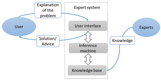
Figure 1.
Architecture of expert system. Adapted from Maylawati et al. [91], and Salman and Abu-Naser [88].
3.2. Genetic Algorithms(GAs)
GAs are one of the evolutionary algorithms using computational models of natural evolutionary processes in developed computer-based problem-solving systems [92]. This system imitates the process of natural genetics and biological mechanisms. It can be used to optimize an objective function, comprehend model prediction and behavior, and determine patterns and relationships, in addition to driving certain phenomena [93].
3.3. Chemometrics
Chemometric approaches are widely used in analytical chemistry, in particular environmental studies, showing the potency of data processing techniques in this field. Quantitative chemical analysis, environmental quality assessment monitoring, modeling, and prediction of toxicological effects are the major areas of interest in chemometric environmental studies [94,95]. The high potential of chemometrics resides in obtaining reasonable analytical results from poor quality of data: low resolution, strong signal overlapping, high level of noise, etc. [96]. Moreover, chemometric techniques improve sensitivity and selectivity, and lower the detection limits of analytical tools. Data description and visualization, detection of hidden relations between analytical signals and sample parameters, discrimination, classification, regression, and prediction are also performed using chemometric tools [97]. Furthermore, chemometrics suggest solutions for complex problems by providing pattern recognition of chemical profiles of environmental or food samples, frequently containing a number of markers to identify [98].
There are many chemometric techniques, such as: Principal Component Analysis (PCA), Partial least squares regression (PLSR), Cluster Analysis (CA), Linear Discriminant Analysis (LDA), Random Forest (RF), etc. These techniques are classified as supervised or unsupervised tools [99].
3.3.1. Unsupervised Methods
These are widely used in exploratory analysis of the global structure of a dataset, and in finding trends and patterns within the dataset. In terms of classification or discrimination of samples, these methods should not be misused. Principal Component Analysis (PCA), Hierarchical Cluster Analysis (HCA), and Partial Least Squares Regression (PLSR) are the most frequently used [100].
Principal Component Analysis
PCA is considered as the most powerful and popular chemometric technique, and is the basis of several other chemometric methods. This approach is a multivariate statistical method usually used in exploratory data analysis [101]. In general, all the data intended for processing are compiled in a matrix form (called X). Each row of this latter matrix contains raw data (variables) in order to describe each studied sample. The PCA is the decomposition of the X matrix with n rows (samples) and p columns (variables) into the product of scores matrix T and transposed loadings matrix P plus residuals matrix E (Figure 2). The scores are the position of the samples in the space of the principal components (PCs) while the loadings are the contributions of the original variables to the PCs [102]. In order to simplify structures and illustrate a large amount of data, PCA is used to calculate a smaller number of possible meaningful linear combinations (PCs) from a large number of variables [103]. Moreover, it permits the dimensionality reduction of data without a significant loss of useful information; exploration of hidden data structure; selecting the significant analytical signals; and clarifying the interrelation between samples and variables [102]. In terms of quantitative analysis of multivariate data, PCA is highly recommended as first instrument [104]. Compared to other multivariate regression tools which are not widely applied, PCA is the most beneficial tool [104,105].
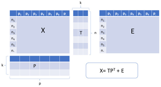
Figure 2.
Schematic representation of Principal Component Analysis where X: raw data, T: Scores matrix, P: Loadings matrix, E: Residuals matrix. Adapted from Panchuk et al. [105] and Dupont et al. [106].
Partial Least Squares Regression
PLSR is an approach that generalizes and combines features from PCA and multiple regression to relate a descriptor matrix (called X) to a prediction vector/matrix (called Y). Afterwards, these two matrices are projected to a new space in order to find the common relations between them (X and Y), leading to a linear regression model. Thus, it aims to predict or analyze a set of dependent variables from a set of independent variables or predictors. In addition, PLSR is considered as a powerful linear regression method, capable of handling collinear variables, and accepting a huge number of variables [107,108]. PLS loadings are able to indicate a group of chemicals that co-vary with the given sample properties; also, by attributing qualitive results, PLSR can be used for discrimination [109,110].
Hierarchical Cluster Analysis
HCA is a method that involves the assessment of similarities between the samples based on their measured properties (variables). According to their adjacency in multidimensional space, the samples are grouped in clusters, and the results are shown in the form of dendrograms to facilitate the visualization of the relationships between the samples [111]. This method is suitable for posteriori data explorations [112]. Unlike PCA, HCA is frequently applied to determine similarities within several groups. These similarities are calculated using different possibilities, such as the correlation coefficient, the Euclidean distance, or the Mahalanobis distance [104].
3.3.2. Supervised Methods
Supervised techniques are based on the prior known data structures that are used to mold patterns and rules in order to predict new data. The advantage of supervised methods is the predictive capability of the models that can be easily used over a new sample. Supervised techniques can be performed by linear methods such as Partial Least Square Discriminant Analysis (PLS-DA), Linear Discriminant Analysis (LDA), or non-linear methods for instance Random Forest RF and Support Vector Machine (SVM), etc. [99,113].
Linear Methods
LDA uses the original variables as a basis in order to come up with a linear function, which maximizes the ratio of between-class variance and minimizes the ratio of within-class variance [114]. Since parameter optimization is not required, LDA is considered as a fast and powerful method to use in discriminant analysis [115].
PLS-DA is a combination of PLS regression and LDA, and is considered as the most popular supervised method used for classification in chemometrics [116]. By checking the behavior of variables, PLS-DA is able to afford excellent insights into the origin of discrimination. Furthermore, it can handle collinear data and is widely applied in modeling and biomarker discovery [117].
Non-Linear Methods
Kernel based models have been used to transform non-linear problems in the original data into a higher-dimensional feature space using particular functions called kernels. Subsequently, the non-linear problem becomes linear and can be solved readily [118]. kernel Fisher discriminant analysis (K-FDA) [119], kernel PLS (K-PLS) [120], and kernel OPLS (KO-PLS) [121] are kernel-based classification methods that have a high potential in solving non-linear problems.
SVM is a kernel-based classifier used to define decision boundaries and separate binary classes using support vectors [122]. This approach is centered on finding a hyperplane that splits two classes perfectly. Whereas the thickness of the margins is maximized, the distance of the plane to the data point is the closest for each class [123,124]. SVM is more suitable for data of small sample sizes. However, SVM-based models suffer from the lack of transparency, and variable importance is difficult to obtain. In addition, this method does not provide a universal means of solving non-linear problems [125].
RF is an extremely efficient classifier for high-dimensional data. It is an ensemble-learning method that consists of a large number of classification and regression trees (CART) [126]. Classification trees are constructed based on training samples selected from the original samples by using a random resampling method with a replacement called bootstrapping. This latter is executed several times to build a large group of simple CARTs [127,128]. Compared to other classifiers, such as PLS-DA, RF has shown better performance, and could be an alternative to PLS-DA [129].
3.4. Artificial Neural Networks (ANNs)
A neuron is a cell that receives, manages, treats and delivers information using biochemical reactions. The human brain is a network formed by more than 10 billion interconnected neurons [130]. ANNs have been initiated as mathematical models simulating the nervous system. Simplified neurons were first introduced by McCulloh and Pitts, thus giving birth to neural networks [131].
Artificial Neural Networks can be defined as biologically inspired computer programs aiming to mimic information processes in the human brain. They are considered as a potential modeling technique, especially for data sets having a complex nonlinear relationship between dependent and independent variables [132]. ANNs are trained through knowledge collected from experiences used as inputs, unlike other techniques which perform specific tasks by simple implementation on a computer [133,134]. After training, new patterns can be used for a specific goal such as prediction and classification without a programming step [5]. Despite the fact that one neuron can execute simple information processes, the main advantage of ANNs, making them a powerful computational tool, is in connecting neurons in a network [135]. Because of the billion interconnections between neurons, ANNs can be easily used to recognize a large variety of input patterns. According to Ferentinos et al., ANN systems allow high-quality, rapid and high capacity of detection [136]. Moreover, they have been applied as a potential method for monitoring and assessment of environmental pollution [136,137].
3.4.1. ANN Architecture
ANNs are basically constructed of three layers; input, hidden and output layer. The first is made of a set of neurons used to receive external data and represent it to the neural network. In general, these inputs are normalized referring to the thresholds produced by activation functions. The hidden layer, also called the intermediate or invisible layer, is responsible for extracting patterns by analyzing processes and systems. The last layer of neurons is responsible for producing and presenting the final output [138,139,140]. Each layer is formed by artificial neurons called processing elements (PEs) that are interconnected, with links to simulate synapses. Each link or weight represents an adjustable coefficient used to moderate combination of input signals, transfer function and outputs [134,141]. Inputs are firstly multiplied by the weights, and then combined and passed through a transfer function to generate the output of that neuron. As biological neurons, artificial neurons can be excited or inhibited by the inputs. Excitatory inputs cause the summing mechanism of the next neuron to add, while the inhibitory inputs cause it to subtract [135]. Sigmoid function is the most frequent transfer function used, while a learning algorithm is used to adjust the weights in order to optimize the learning accuracy of the PE [142].
ANN can be composed of a single layer, leading to a simple neural network, or multiple layers leading to a multilayer neural network. The simple neural network is especially adapted for simple problems, while the multilayer neural network is principally used for more complicated processes [142]. A simple artificial neuron and a multilayered artificial neuron network schemes are illustrated in Figure 3 and Figure 4, respectively.
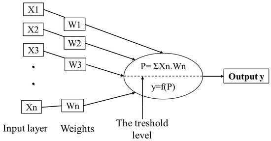
Figure 3.
Architecture of a simple artificial neuron. Adapted from Agatonovic-Kustrin and Beresford [137] and Abraham [142].
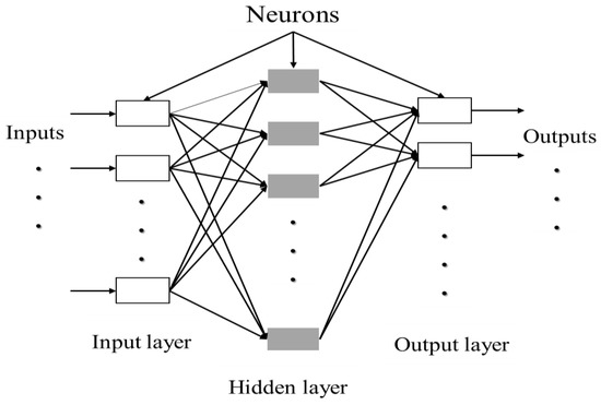
Figure 4.
Architecture of a multilayered structure of artificial neural network. Adapted from Abraham [142].
ANNs’ process and behavior are highly affected by neuron connection. Based on this, ANNs can also be categorized into two groups: feed-forward networks and feedback or recurrent networks [143].
Feed-forward networks are considered as a static system; there are no loops (absence of feedback) or connections from output to input neurons. The signals are transmitted in one direction only from inputs to outputs. Therefore, outputs of the previous operation are not memorized and the next one depends only on the input signals (memory-less) (Figure 5) [144,145]. This type of architecture can be structured as monolayer or multilayer composed of one or more hidden neural layers [137,140].
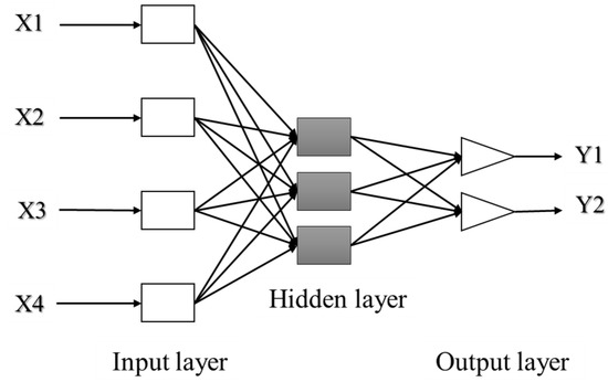
Figure 5.
Feed-forward network structure. Adapted from Agatonovic-Kustrin and Beresford [137].
Recurrent (or feedback) networks are considered as a dynamic system where loops are formed as a result of connections from output to input neurons(loops). In this case, the outputs of neurons are used as feedback inputs for other neurons. Such a network system memorizes the previous state, so that the next state depends not only on input signals but also on the previous outputs (Figure 6) [135].
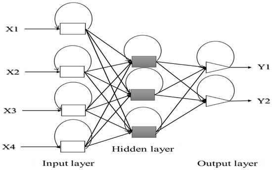
Figure 6.
Feedback network structure. Adapted from Agatonovic-Kustrin and Beresford [137].
Other architectures have also been also described in the literature, such as the Elman network, adaptive resonance theory maps, and competitive networks. In general, the architecture is selected based on the properties and requirements of the application [137]. In parallel, following the type of network and training algorithm, different activation functions may be used: logistic sigmoid, linear, threshold, Gaussian or hyperbolic tangent functions [146].
3.4.2. Learning Rules
After selecting the adequate network, a training step is required to produce the desired outputs at the suitable time, hence the importance of adopting a restrictive learning rule. Learning rules are different from ANN models; ANN models represent the arrangement and the disposition of neural networks, while algorithms compute the output. A learning rule is defined as any systematic adjustment of weights that minimizes error function or maximizes a specified benefit function. This means the ANN’s recognizing abilities are based mainly on weighted links [147].
Two main rules can be adopted for training: supervised and unsupervised algorithms [135]. Fully connected, supervised ANNs with back propagation learning rule are the most popular, in particular for prediction and classification. In parallel, the Kohonen or Self Organizing Map with unsupervised learning algorithm is highly used for finding complex relationships among data [137].
Supervised algorithms: This rule is based on the relation between the inputs and outputs of a training set. By using this type of algorithm, the network generates the desired output for every input data. Errors between the obtained values and the known ones in each output layer nodes are first calculated. Then, these errors are used by the learning rule to determine proper weights giving suitable results and a high quality of prediction [148]. It has been reported that the number of hidden neurons must be optimized, otherwise a system failure can occur decreasing prediction abilities [137,148].
Unsupervised algorithms: This rule requires a training task to classify input patterns into different categories according to the correlation between them [149]. It consists of an auto-organized system, since features are selected by the system itself to categorize the input data and achieve a specific classification. This system behavior implies competition between neurons, co-operation, or both [137,142,148]. For competitive learning, among a group of neurons, the one responding strongly to the input will inhibit the other neurons. For co-operative learning, neurons of each category work together to enhance their outputs [137].
Hybrid learning: is a mixture of supervised and unsupervised learning, which are combined to determine weights [140].
Reinforcement learning: This type is a variant of supervised learning based on the correctness of network outputs. This learning rule requires a reward for a correct output and a penalty for the wrong one [140,150]. Trial and error research and delayed reward are the two major special features of reinforcement learning [142].
Error-correction rules: During the learning process, an error correction rule is used to calculate the difference between the desired and the obtainedvalues. The aim is to adjust the connection weights and gradually reduce this error [149].
Hebbian rule: Almost all neural networks’ learning techniques are considered as a variant of the Hebbian learning rule, since it is the oldest learning rule based on the observations of neurobiological experiments [151]. The interconnection of two neurons has to be enhanced if the two neurons are stimulated at the same time. However, in the case of a single layer, one of the interconnected neurons will constitute the input unit while a second one forms the output unit [142].
3.4.3. Training and Testing Neural Networks
The best way to ensure the efficiency of ANNs is to execute a number of problems with different characteristics. The adjustment process or training aim to adjust weights and threshold to obtain output values close to the desired ones. The number of these trainings is determined by the complexity of the samples. During training, some noises can be added to enhance the system applicability in real samples [148]. Poor training data generates an uncertain network, while an overtraining generates a system unable to make execution outside of the training set. Other parameters have to be considered, such as the number of nodes in the hidden layer which plays a key role in the network functionality. Using many nodes in the hidden layer will increase the number of possible computations of the algorithm, while just a few nodes in the hidden layer can prevent the algorithm from learning. Therefore, the right balance needs to be picked [146]. In parallel, selecting initial weights is crucial, in particular for multidimensional ones. This can be obtained by testing different initial weight values to attain the desired results. Finally, the system performance is also affected by the learning rate since it controls the size of each step [142,148].
3.5. Modern Computational Approaches
These approaches are widely used to screen and classify the design/shape of bioreceptors and forecast the resultant interaction. Since computational approaches are based on computational calculations, they have anultra-sensitive and selective potential. In this context, computational docking and molecular dynamics (MD) are two common techniques based on numerous algorithms and used to predict the interrelation receptor–ligand.
Computational docking is a promising approach aiming to enrich experimental structural data on receptor–ligand interactions and optimize the conformation and the quaternary structure of the formed complexes [152,153]. These techniques are based on placing a small molecule in the specific binding site of its macromolecular target with an estimation of the binding affinities [154]. The docking process involves two main approaches; sampling and scoring, that can be coupled together or occur in different stages [155]. Sampling is a search process that generates different possibilities of binding orientations and/or conformations (i.e., modes) between two molecules within the constraints of the receptor binding site. Scoring is the computation, using the score between two molecules in a binding mode. Afterwards, the binding modes are ranked according to their binding scores, and the best ones can be selected as the final docking solutions (ligand conformation, orientation, and translation) [156,157].
Molecular dynamics is an established simulation tool in biomolecular study, offering information about the hydrodynamic behavior [158,159]. It is based on modeling molecular structure using potential-energy functions. In other words, MD simulations involve the iterative numerical calculation of instantaneous forces present in the system, a set of particles that move in response to their interactions according to a defined equation, and the consequential movements in that system. This approach is principally used to obtain data in the precision and evolution of molecular conformations, but also kinetic and thermodynamics information [160]. Moreover, this dynamic simulation method is used to clarify the interaction mechanism quantitatively and qualitatively [161]. In term of environmental monitoring, these computational techniques have been used to redesign and model essential enzymes (organo-phosphatase) for pesticide hydrolysis, to reactivate their unexploited catalytic potential, and to determine their mode of action [162,163].
4. Application of Artificial Intelligence in Environmental Biosensing
Monitoring the environment via biosensors is based on two approaches; affinity-based sensing where pollutants can be detected by a highly specific receptors, i.e., antibodies or aptamers which may come at a cost; and inhibition sensors, particularly based on enzymes that are inhibited by pollutants [164]. The enzymatic approach is much simpler and less expensive but the receptor may be affected by other pollutants, influencing sensitivity and selectivity. Therefore, sensors based on more than one bio-receptor have to be used for the simultaneous detection of different analytes. To achieve this, the cross-disciplinary concept of AI is more than a necessity. AI-based biosensors are based on three elements: information collection, signal conversion and AI-data processing. Information collection refers to regularly monitoring physical, chemical, biological, or environmental information using biosensors. The signal conversion aims to generate an electric output, with a defined sensitivity, from the collected information. Finally, AI-data processing comprises interface, data classification, data model and analysis, and decision layer [165,166].
4.1. Environmental Monitoring Based on Chemometric Methods
Chemometric methods are extensively used in environmental monitoring as they permit the identification and description of the interrelations between environmental factors. In addition, they clarify the potential impact of these factors on the environment [167].
A chemometric approach was used to get a better insight into some trace metal patterns. The concentrations of Cu, Zn, Mn, Fe, K, Ca, Mg, Al, Ba and B in 26 herbal drugs were studied using flame atomic absorption and emission spectrometry, as well as inductively coupled plasma atomic emission spectrometry. Afterwards, a PCA was used to highlight the relation between the elements. Four significant factors were identified and partly attributed to the significant influential sources and high mobility of some elements, thus referring also to potential anthropogenic contamination. In this work, of all chemometric methods the PCA is the most suitable because it allowed the identification of factors that are substantially meaningful [168]. In contrast to the previous work which was based on one chemometric technique, this research group used three chemometric techniques (PCA, LDA and cluster analysis). In this study, they evaluated trace metal concentrations (As, Ba, Ca, Cd, Co, Cr, Cu, Fe, Mg, Mn, Ni, Sr and Zn) in spices (black pepper, chili pepper, cinnamon, cumin, sweet red pepper and turmeric) and herbs (mint, thyme and rosemary). They used an atomic spectroscopy for the determination of trace metals, and chemometric evaluation for the classification study. As a result, herbs and spices were classified into five groups by PCA and CA. Compared to the results obtained by LDA, it was found that all group members determined by PCA and CA are in the predicted group and that 100% of original grouped cases are correctly classified by LDA [169]. Chemometric methods are also used to evaluate phenolic compounds. In this context, phenolic and flavonoid compounds are identified in four unifloral honey types using chemometric approaches (PCA and HCA). Moreover, the correlation among the physico–chemical characteristics was also studied. The first three PCs explained more than 83% of the variance with minerals showing the highest discriminating power while HCA successfully classified all the unifloral honey samples. This work demonstrated that it is possible to effectively classify honey by applying chemometric techniques (PCA and HCA) [170].
Nowadays, near-infrared spectroscopy (NIRS) is combined with chemometric techniques in order to monitor the environment [171]. A study reported the quantification of pharmaceuticals in wastewater using Fourier transformnear-infrared (FT-NIR) spectroscopy methodology. The samples were treated by chemometric techniques in order to develop and validate the quantification models. The obtained results were found adequate for the prediction ofibuprofen, sulfamethoxazole, 17β-estradiol andcarbamazepinewith R2 around 0.95 and residual prediction deviation values above four. FT-NIR spectroscopy is not used as a direct analysis technique because it suffers from the complexity of the spectra. For this reason the FT-NIR methodology is combined with chemometrics, exploring a promising technology which is able to quantify a wide range of organic compounds [172]. Since lichens are extremely sensitive to the presence of substances that alter atmospheric composition, near-infrared (NIR) spectroscopy was developed as a tool for discriminating between lichen samples exposed to air pollution. In addition, PCA and LDA are used as chemometric methods to successfully discriminate between samples from polluted and non-polluted areas. The PCA was applied in the NIR spectra as a multivariate display method to visualize the NIR data. The LDA was carried out to discriminate between lichens based on their exposure to pollutants. On average, 95.2% of samples were correctly classified, and 100.0% external prediction was achieved. These results showed that NIR-spectroscopy based chemometric methods can be considered as a potential reliable method to support traditional methods for the discrimination between lichen samples according to their exposure to pollutants [173]. Another study based on NIR spectroscopy combined with chemometric techniques was also described as a monitoring tool of exhaust air from poultry operation systems. Samples were collected from the exhaust air of two poultry houses using sophisticated filter sampling protocols. This study aimed to monitor spectral differences caused by the cleaning device, and to follow changes in exhaust air characteristics during a fattening period. PCA, LDA, and FA were successfully used to classify the NIR exhaust air spectra according to fattening day and origin. The results show that the dust load and the composition of exhaust air significantly affect the NIR spectral patterns. These results confirmed that the sample classification according to fattening days, raw and cleaned exhaust air was possible by using chemometric methods [174]. These results demonstrate the high potential of NIRS combined with chemometric techniques to monitor an environment in a non-destructive, quick, and elegant way.
Chemometric approaches are also used to evaluate the influence of seasonal changes in volatile organic compound concentrations [175], to rapidly classify heavy metal-exposed freshwater bacteria [176], and to monitor air and water quality [177,178,179,180].
The combination of chemometrics and sensors is positioned to be a major breakthrough in collecting meaningful data and forits depth of analysis in determining trends and interrelationships [167,171,181,182]. In this context, Lamagna et al., used an electronic nose to analyze samples that were collected above a river basin in Argentina. This electronic nose consisted of 32 polymer sensors used to measure the concentration of SO2 and H2S in the air. The combination of PCA and the sensor was used to identify the sampling sites that deviated significantly from a control sample of clean air. This combination was able to identify a correlation that existed between polluted sampling sites and the electronic nose response, indicating that this system could be used for monitoring pollution in rivers [183]. Another study reported the use of a potentiometricmultisensor systemin order to assess water toxicity in terms of the bioassay with three living test organisms: Daphniamagna, Chlorella vulgaris and Paramecium caudatum. Using a PLS regression from the obtained data, the prediction of water toxicity with relative errors 15–26% was attainable. Further experimental work with larger data sets is required to improve the performance of such “artificial bioassays” [184].
4.2. Environmental Monitoring Based on Artificial Neural Networks (ANNs)
Developing a biosensing system able to detect and quantify several targets simultaneously represents a challenging tool in environmental monitoring. It has been reported that various pesticides, including organophosphorus (OPs) and carbamate insecticides, can inhibit cholinesterase activity. Based on this, several enzymatic inhibition biosensors have been developed [185,186,187,188,189,190,191,192]. However, all have the difficulty in discriminating between different inhibitors. To overcome this problem, biosensing platforms have been conjugated with an ANN to find a pattern relating inhibitor concentrations to the observed inhibition percentages, allowing thus an accurate biosensing [193]. Table 1 summarize some application of ANN in environmental monitoring.

Table 1.
Summary of Artificial Neural Network (ANN)-based biosensing platforms applied to pollutant detection.
4.2.1. Pesticide Monitoring
Several intelligent biosensors based on the principle of acetylcholinesterase (AChE) inhibition and chemometric data analysis using ANNs have been developed [136,194,196,197,217,226]. Istamboulie et al. developed an amperometric acetylcholinesterase biosensor based on ANNs to selectively quantify and discriminate a mixture of pesticides in real water samples using two constructed ANNs. They modeled the combined response of two pesticides (chlorpyrifos oxon and chlorfenvinfos) using sensors incorporating wild-type electric eel AChE and drosophila mutant AChE, associated or not with a phosphotriesterase PTE. A satisfying prediction ability was obtained with correlation coefficients better than 0.986 and a limit of detection of 0.02nM for chlorpyriphos-oxon, and 0.15 nM for chlorfenvinphos [226].
This developed tool used two enzyme variants to detect only two pesticides. Therefore, other biosensors have been described to reduce the number of enzyme variants and detect more analytes. A further investigation was conducted by the same group to generate an array of three biosensors formed by screen printed carbon electrodes and two different AChE enzymes. The developed device was able to discriminate various insecticides with high accuracy. In this work, ANNs were used in combination with the enzymatic activity rate as analytical signal, rather than the inhibition percentage.The simultaneous detection of the three insecticides mixtures (chlorpyriphos-oxon, chlorfenvinphos, and azinphos-methyl-oxon) was achieved successfully by applying only two AChEs from Drosophila melanogaster (wild-type and genetically modified). The obtained results were very interesting in terms of sensitivity and precision with low error, and correlation coefficient higher than 0.985. As compared to the previously discussed work, this method is faster and simpler, allowing the detection of three compounds [196]. Based on the same principle and using a spectrophotometric assay with three different enzyme systems, the detection of more than two pesticides has been carried out. This system was successfully applied to resolve the three insecticides chlorpyriphos, dichlorvos and carbofuran in real water samples, with high correlation coefficients of, respectively, 0.916; 0.991; 0.959 [198].
Later, Bachmann and Schmid developed, for the first time, a highly sensitive screen-printed amperometric multielectrode biosensor for the rapid quantification and discrimination of paraoxon and carbofuran in insecticides mixture. They used four types of native or recombinant AChEs as specific ligands by combining the AChE-multisensor with feed-forward ANNs for quantitative inhibition analysis of the binary mixture. The prediction errors were 0.9 mg/l for paraoxon and 1.4 mg/l for carbofuran with apparent Michaelis–Menten constant, Km of 0.08 mM. This multi-sensor achieved a LOD of 0.2 µg/L which is much lower than that obtained in other reports [195].
In another report, Schäfer et al. described a high potential assay for the specific detection of organophosphorus compounds and carbamates incorporating extensive chemometric data analysis using soluble AChE in the microtiter plate method. In contrast to the biosensors described above, this assay procedure is restricted to laboratory use only [227].
Crew et al. went a step further and presented a portable analytical system integrating an array of six AChE-based enzymatic biosensors in a novel automated device equipped with an efficient ANN program. This analytical tool was used to successfully resolve a mixture of 6 pesticides, dichlorvos, malaoxon, chlorpyrifos-oxon, chlorpyrifos-methyl-oxon, chlorfenvinphos and pirimiphos-methyl-oxon from nM to mM concentration range, in less than 6 min. In addition, the system was also validated for different sample matrices, including water, food and vegetable extracts, without false positives or negatives (Figure 7) [228]. Finally, several reports have also described the ANN-assisted biosensing of dipterex, dichlorvos, methyl paraoxon, and omethoate [194,196,201,229]. A cell-based biosensor incorporating ANNs was also established to classify pesticides into different groups (pyrethroids, carbamates and OPs) [136].
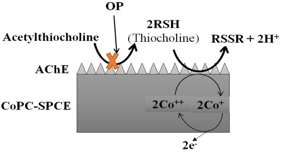
Figure 7.
Schematic diagram explaining the principle of the reactions based on this amperometric biosensor. Adapted from Crew et al. [228].
4.2.2. Heavy Metals Monitoring
In addition to pesticides, heavy metals biosensing constitutes a great challenge in environmental monitoring. ANNs have been used for soil and water studies, such as predicting contamination, measuring organic content and macronutrients, pollutant infiltration properties and soil classification [205,206,214,230,231,232,233,234].
A sorption model was developed by Anaguet al. for the estimation of heavy metals sorption from basic soil properties and evaluating the risks related to their apparition. In this work, nine heavy metals have been targeted; Cd, Cr, Cu, Mo, Ni, Pb, Sb, Tl, and Zn. The ANN models showed a high performance with a root mean square error (RMSE) ranging from 0.04 µg·kg−1 (Cd) to 0.1 µg·kg−1 (Cr) and a modelling efficiency (EF) ranging from 0.79 (Cr) to 0.94 (Cd, Zn). By comparing these results to those based on multiple linear regression (MLR), we can conclude that ANN models behave better than MLR, where EF ranged from 0.03 to 0.13 [205].
ANNs have also been combined with electrochemical biosensing platforms for HM detection in the environment, by using various types of electrodes. For instance, an electronic tongue approach based on polyvinyl chloride (PVC) membranes has been used in the rapid and simple on-site monitoring of several heavy metals [210,235,236,237]. In this context, a mixture of three heavy metals (Pb2+, Cd2+and Cu2+) have been resolved using an e-tongue (ANNs) integrated with a membrane selective electrode. A limit of detection of 1mg·L−1was attained for the three targets with a good reproducibility. In addition, the correlation was significant for the three ions, exceeding 0.975. Finally, this system showed a good prediction ability when applied to contaminated soil samples [207]. Despite the interesting resulting, this strategy is adapted only for three HMs. Therefore, another group investigated the simultaneous detection of a mixture of four HMs by using the same principle of potentiometric e-tongue and PVC membranes using ANNs. The method was successfully applied for the quantification of low levels of Cu2+, Pb2+, Zn2+, and Cd2+ ions from quaternary mixtures in soil, open-air waste streams and rivers with low root mean squared error values (~1 mmol·L−1) [210].
Besides PVC membranes, other electrodes have been used in ANN-based sensing of heavy metals. A research group investigated the resolution of a mixture of Pb, Cr, Cu, Cd and chloride ions by using a flow injection set-up method with multiple chalcogenide glass chemical sensors (electrodes). For this, seven electrodes were constructed and the output signals were analyzed using multivariate analysis method including artificial neural networks. The detection limit for Pb was about 3 μM and about 1 μM for the other metals. Besides, the chloride ions can be determined down to about 1 μM alone, and 20 μM simultaneously with other pollutants. The average error for metals resolution in the scale from the detection limit went up to about 3 mM, with 10–15% for the metal mixture, and about 30% for Cl− [208]. In another report, a graphite epoxy composite electrode wasused to detect a quaternary HMs mixture using a specific type of voltametric detection method. In this work, for the first time, a three-sensor array was applied for the simultaneous quantification of Cd (II), Pb (II) and Hg (II) ions in certified samples. They used two graphite epoxy composite electrodes modified with carboxybenzo (CB)-18- crown-6 and CB-15-crown-5, respectively, and an unmodified one. The crown ethers serve as molecular collector with ability to selectively coordinate with the metal ions for complex formation by means of ion-dipole interaction with metal ions. The expected and the obtained results were very close and the achieved LODs and limits of quantification (LOQs) were at levels of µg·L−1. These results confirmed that this biosensing array provides a discrimination power to resolve HM mixtures [209]. Other studies devoted to the application of crown ether-modified electrodes for the simultaneous determination of individual/mixture HMs have also been reported [238,239,240,241,242].
Finally, electrochemical biosensing technologies based on ANNs seem to be successfully adapted for the simultaneous detection of EP mixtures in the environment at the ultra-trace level. Furthermore, these systems provide several advantages such as high specificity, fast response time, portability, simplicity, and low cost, making them reliable devices for EP monitoring [243,244].
4.2.3. Air and Water Quality Monitoring
Several approaches based on ANNs have been developed for modeling the monitoring of air and water quality or of environmental systems in general [245,246,247,248,249,250,251]. In this context, a statistical model was developed for the accurate forecasting of the Air Pollution Index (API) in industrial and residential monitoring stations in Malaysia. For this, the autoregressive integrated moving average (ARIMA), fuzzy time series (FTS) and artificial neural network were employed. By comparing the obtained results with that of ARIMA and FTS, the ANNs exhibited the smallest error in forecasting API values. This method thus constitutesan effective way to control the air quality and for decision-making processes [252]. Later, Wang et al. [253] studied the causal relationship between urbanization and water quality indices, and used this as a support to predict the water quality. Correlation and path analysis were used to identify the causal relationships, followed by a back-propagation neural network to predict water quality. The obtained coefficients of correlation were higher than 0.76 improving thus the performance of the optimized model for predicting urban water quality with nonlinear variation. However, this work was limited to simulation studies in calculating the API. Another report describing experimental validation of modeling has been published. The authors developed an electrochemical sensor array based on the inhibition of immobilized bacteria for the preliminary detection of a wide range of organic and inorganic pollutants. The objective of this work was based on heavy metal salts, pesticides, and petrochemicals monitoring in water using three types of bacteria, namely Escherichia coli, Shewanellaoneidensis, and Methylococcuscapsulatus. The response of each pollutant was monitored with more accurate recognition using the ANNs. The obtained system was capable of resolving all these pollutants at low concentrations (down to 0.1 μM) [254].
4.2.4. Pharmaceuticals Monitoring
Several electrochemical biosensors assisted by ANNs have been developed for therapeutic substances detection, in particular phenolic compounds mainly based on tyrosinase (Tyr) and laccase (Lac) [255]. Gutéet al. developed an electrochemical biosensor combined with ANNs to simultaneously detect different phenols (phenol, catechol and m-cresol). A single graphite epoxy bio composite bulk-modified with Tyr was used in combination with a sequential injection analysis (SIA) system. Departure information was extracted via the whole voltammogram, and then ANNs were used for extraction and quantification of each compound. The model of the three analytes shows a good correlation coefficient: phenol 0.988; catechol 0.997; and m-cresol 0.993 [165]. In this study, the authors compared the obtained results with that of a previous study reported by Trojanowicz et al. [256], based on the same principle, by using only the steady-state responses rather than the whole voltammogram. The authors confirm that the results of this method were not performant with low correlation coefficients between expected and predicted values. Therefore, they attributed this to the lack of the data afforded by the system. Later, another biosensor based on the same principle and on three composite electrodes bulk-modified with tyr, lac, and copper nanoparticles has been developed for the simultaneous monitoring of catechol, m-cresol and guaiacol in wastewater. The method was based on a voltametric bioelectronic tongue where the electrochemical responses of the three composite electrodes were compressed by means of fast Fourier transformation. Each voltammogram was compressed down to a number of coefficients which were used as inputs to the ANN model. The system was also applied for the photo-degradation monitoring of the three phenolic pollutants. This proposed approach exhibited a good correlation coefficient with a RMSE of 1.50 for the training subset and 4.20 for the testing subset. These results showed the powerful potential of this approach for the speciation of different phenolic compounds in wastewater and the monitoring of its mineralization. Moreover, using this approach, a quantitative multi-determination of a mixture of chemical species can be easily attainable with simple equipment, shifting the complexity from the sensors to the software side [219]. Later, Boroumand et al. reported the flow injection simultaneous kinetic determination of two isomers, Hydroquinone and catechol. In this work, a simple FIA manifold equipped with double injectors and single detection system was combined with a Bayesian Regularized Artificial Neural Network for determining the targets in real samples. Detection limits of 0.05 and 0.07 mg·L−1 were obtained for HQ and CC, respectively [216].
4.2.5. Biotoxins Monitoring
The great potential of ANNs for resolving multivariate calibration problems has been also explored for biotoxins analysis. For instance, Saidi et al. reported the rapid determination of OTA by a spectrofluorimetric procedure-based ANN. The study described the application of the ANN method to a set of spectrofluorimetric data obtained from the analysis of wheat and rice samples contaminated with OTA. The obtained results were significant with a correlation coefficient of 0.995 and a mean square error of 0.036 [79]. Another method using an electronic nose equipped with a 10-metal oxide sensor array has been subsequently reported based on a set of data collected over five years. This e-nose array allowed the rapid identification of aflatoxin B1 and fumonisins in maize samples using three different statistical approaches: ANN, logistic regression, and discriminate analysis. Notably, ANN gave better results than the other methods, with 78% and 77% accuracy for AFB1 and FBs, respectively. In contrast to certain strategies [257], the majority of the data set in this work were collected over five years and analyzed in different ways providing, thus, a remarkable reliability [258].
Another model based on artificial neural network was developed to estimate blue-green algae fluorescence for the year-round data collected in 2016–2017 from western Lake Erie, USA. Eight input parameters including phosphorous, nitrogen, chlorophyll-a, air temperature, water temperature, turbidity, wind speed, and pH were used to run the model. Five different learning algorithms were tested, and among these the Levenberg-Marquardt algorithm gave the highest R2 values of 0.98 and 0.72 for the eight and three (phosphorous, nitrogen, and chlorophyll-a) input parameters, respectively. Based on this, the best estimation of blue-green algae fluorescence was achieved using eight input parameters while a weak correlation was obtained with the three input parameters. This method allows the rapid and low cost prediction of blue-green algae by using simple measurements [259].
4.3. Environmental Monitoring Based on Genetic Algorithm (GA)
Genetic algorithm plays an important role in environmental monitoring, particularly, in optimizing the quality of the developed systems, improving thus the final results [260]. Table 2 summarize some application of GA in environmental monitoring.
Table 2.
Summary of genetic algorithm (GA) applied to pollutants detection.
Karkra et al. have applied genetic algorithm to 24 water samples containing eight different heavy metal ions (Cd, Co, Zn, Ni, Cu, Cr, Ag and Pb). The goal of this study consisted in selecting the optimal electrode as well as the corresponding frequency allowing the classification of heavy metal ions. Different electrodes including gold, platinum, glassy carbon and silver nanoparticles were tested in combination with different frequencies. Genetic algorithm was used to select the electrodes giving the best combination. In parallel, GA provided the best clustering indexes, a similarity index of 0.599, Davies-Bouldin index lower than 0.112 and a sufficient value of dissimilarity index which confirms the significant distance between the formed clusters. Based on this study, various hazardous metal ions present in the tested water samples have been optimally classified. However, this system is more complex as it uses multiple electrodes, thus increasing the time and cost of fabrication [266]. Apart from HMs, genetic algorithm has been also used for the monitoring of other pollutants. Carreres-Prieto et al. have developed a spectrophotometry-based statistical model to estimate chemical oxygen demand (COD), biological oxygen demand at five days (BOD5), total suspended solids (TSS), phosphorus (P), total nitrogen (TN) and nitrate nitrogen (NO3−,N) of both raw and treated water without the need for any pre-treatment or chemicals. Multivariate linear regressions and machine learning genetic algorithm have been used to measure the spectral response of wastewater samples based on the absorbance and transmittance in the UVnear visible and visible 380–700 nm wavelength range. The obtained results have shown that the multilinear regression models can estimate only COD and TSS of raw water with less than a 0.5% error rate. In parallel, the models elaborated by means of GA can predict the degree of five pollutants (COD, BOD5, TSS, TN and NO3−N) in both raw and treated wastewater with an error rate below 4% [264]. In contrast to the previously reported water quality assessment methods based on a single wavelength [267,268,269,270], the use of genetic algorithm, in this work was based on multiple wavelengths (81 wavelengths). Therefore, it improved the estimation accuracy of the pollution load of wastewater.
Other studies investigated the combination of Partial least squares (PLS) with genetic algorithm to extract pertinent information and produce truthful models. Nowadays, the PLS concept is applied by several researchers, according to Martens and Nea’s algorithm [271,272]. However, the choice of wavelength would critically affect the future predictive ability of the model. To overcome this problem several selection methods have been developed, e.g., artificial neural network [273], Tabu search [274], hybrid linear analysis (HLA) [275], successive projection algorithm (SPA) [276], and genetic algorithm. In this context, a simple, fast and accurate procedure for quantifying malathion has been developed. Attenuated Total Reflectance-Fourier Transform Infrared (ATR-FTIR) spectra were used to select a specific region for the quantitative analysis using partial least square (PLS) and two wavelength selection methods: principal component regression (PCR) and genetic algorithm. Then, the relative error of prediction was calculated: 3.536, 1.656 for PLS and PCR-PLS, respectively, and 0.188 for GA-PLS, with correlation coefficient of 0.999. Based on this, we can say that GA can be considered as a helpful wavelength selection method for better capability of prediction [261]. Later, genetic-algorithm-based wavelength selection in multicomponent spectrophotometric determination by PLS was developed to detect a mixture of zinc and copper without a pretreatment. The method was based on the reaction between the analytes and a chromogenic reagent (2-carboxy2′-hyroxy-5′-sulfoformazylbenze (Zincon)) at pH 9. A series of synthetic solutions containing different concentrations of copper and zinc were used to check the prediction ability of the GA–PLS models. The root mean squares difference (the average error in the analysis) for copper and zinc with GA and without GA were 0.0407 and 0.0865, 0.2147 and 0.3005, respectively. Despite the high spectral overlapping observed between the absorption spectra of the mixture components, the obtained results proved the high potential of this approach to overcome the spectral interferences and detect simultaneously the cited ions in natural, tap and waste waters. Another pertinent point is that the selected variables clearly identify spectroscopically relevant regions, which demonstrated also the utility of GA for feature selection in a spectral data set [263].
In a recent study, Sajadi et al. used modeling and simulation of chemical reactions to construct a potentiometric AChE biosensor of Aflatoxin B1 by determining the optimal reaction rate constants. Enzymatic reactions were simulated using COMSOL software while reaction rates were optimized by ANN and GA. This method has shown satisfactory results with Mean Absolute Percentage Errors equal to 0.7074%, 0.9458%, 0.7473% and 0.7492% for train, validation, test and total data sets, respectively, and correlation coefficient higher than 0.999. As compared to the results obtained with other models used for predicting AChE enzyme inhibition by AFB1 [277,278], these results showed that trained Neural Network using Genetic Algorithm optimized reaction rates, exhibiting the lowest MAPE [224].
4.4. Environmental Monitoring Based on Expert System (ES)
In addition to genetic algorithm, expert systems are also used for environmental pollutants monitoring. An expert system devoted to voltametric methods for determining mercury (Hg), vanadium (V), and selenium (Se) has been developed. This work was an improvement on a previously described expert system for the determination of Cu, Zn, Cd, Pb, In, Ni, Co, Tl, Hg, V and Se, at trace levels [279,280]. The expert system was developed using a knowledge engineering system, in order to guide the user to choose the sample treatment and the most appropriate voltametric procedure for the identification and the quantification of the three trace metals. Four techniques were implemented: differential pulse polarography, anodic stripping voltammetry, cathodic stripping voltammetry and adsorptive stripping voltammetry, using mercury drop electrodes and a gold electrode. The authors demonstrated that the reported technique constitutes a very useful and reproducible approach, in particular for non-expert users in this field [281]. Based on ES, advanced mathematical techniques have also been designed in order to manage water quality monitoring networks. These studies include the development of a software tool for decision support, based on the application of fuzzy logic techniques and using the experience and knowledge of experts in this field. This system indicates water quality episodes from the behavior of variables measured at continuous automatic water control networks, which can hardly be detected by discrete sampling. Based on the recorded variables, the expert system provides different water quality phenomena indicators. These latter may be associated with a high probability of cause-effect relationship including human pressure on the water environment, urban discharges, or agricultural diffuse pollution. These indicators will forecast and complete manual sampling and laboratory analysis. Besides, this study demonstrated the ability of the expert system based fuzzy-logic to synthesize complex information, interpreted only by a few performant experts, and translated it into more understandable indicators for non-expert users [282].
In the literature, few reports have described ES in environmental monitoring, which can be explained by the necessity of deeper levels of understanding, interpretation, and expertise in the overall processes. The lack of knowledge available for a process leads to complex codification, in particular for activities that involve significant amounts of pattern recognition, generalization, and use of analogy [283]. Since an increasing number of researchers emphasize hybrid methods instead of single ones, more efforts should be focused on the use of ES combined with other strategies to involve contextual perspectives and develop high-quality models to monitor the environment [284,285].
4.5. Environmental Monitoring Based on Computational Approaches
In term of monitoring the environment, computational approaches have been explored to develop/redesign new bioreceptors or to reactivate biocatalysts for reactions of interest [152,162,286].
Computational approaches have been used to simulate a specific aptamer for diazinon, by studying molecular behavior and complex stability. The best sequence exhibiting a high affinity to bind Diazinon, was selected among twelve aptamers isolated from SELEX experimentation. Initially, Jokar’s team used a docking technique as first virtual screening to select the most frequent conformation of each aptamer. Then, the docking results were used as inputs to molecular dynamics for a secondary screening. MD allows the simulation of the quantity and quality of aptamer–diazinon interaction, pointing out the conformational flexibility. In addition, it highlights the bonding interactions between diazinon–aptamer complexes showing the important role of binding energy in reinforcing this complex. Computational screening and analytical results showed that G-quadruplex DNA aptamer (DF20) with its stable complex, low oscillation, shifting toward folded states and high ratio of H-bond aptamer-Diazinon was the reliable candidate for diazinon biosensing. Based on simulation results, a colorimetric biosensing platform was constructed for the ultrasensitive detection of Diazinon in the range of 0.141–0.65 nM with a LOD of 17.903 nM. Finally, the AuNPs-apta-sensing strategy was validated using a computational molecular approach. These computational approaches provide thus a promising alternative to laboratory experiments for receptor structure screening and the prediction of interaction outcomes [152].
Computational techniques also have a great potential application in studies redesigning the essential enzymes for OP hydrolysis and reactions that are not known to be catalyzed by natural enzymes. In this context a computational method has been developed to redesign a mononuclear zinc metalloenzyme for organophosphate hydrolysis. This approach aims to repurpose the reactivity of metalloenzyme active site functional groups for catalyzing new reactions. Based on this principle, Khareet al. engineered a zinc-containing mouse adenosine deaminase to catalyze the hydrolysis of an organophosphate substrate with a catalytic efficiency (kcat/Km) of ~104 M−1·s−1. In the high-resolution crystal structure of the enzyme, all the conception residues adopt the designed conformation except one residue. This computational enzyme design method could be considered as a general approach for exploring untapped catalytic potential for new reactivities [162]. Likewise, an optical biosensor for environmental monitoring has been developed based on protein modelingand computational screening followed by virtualmutagenesisanalyses. This approach was used for the engineering of functional amino acids in the D1 protein of the photosyntheticelectron transferchain of Chlamydomonas reinhardtii. These functions are able to detect two classes of pesticides, triazineandurea. The resulting protein was subsequently used to develop an optical biosensor for environmental monitoring with limits of detection between 0.8 × 10⁻¹¹ Mand 3.0 × 10⁻⁹ M, depending on thetarget analyte (Figure 8) [287].
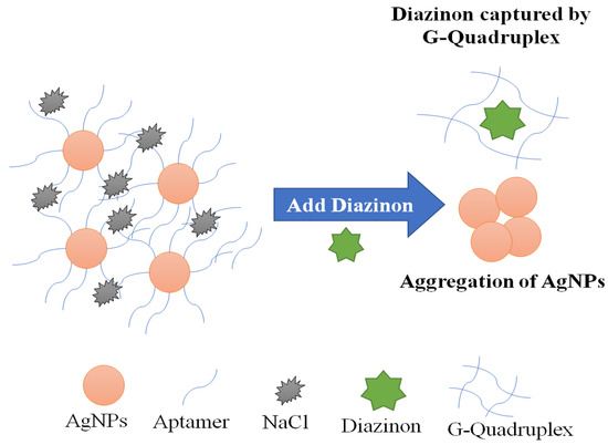
Figure 8.
A schematic representation of the principle of Diazinon colorimetric aptasensing. Adapted from Jokar et al. [152].
Nanoparticles affect negatively living organisms(cytotoxic, neurotoxic, genotoxic, etc.) and environmental ecosystems, and in that sense computational methods have been used as an efficient tool to assess and evaluate the hazardous effects of toxic nanoparticles [288]. Because of the high-cost and time-consuming of the experiments, the quantitative structure–activity relationship (QSAR) method is commonly used to predict the toxicity of different nanomaterials by developing nano-QSAR models [289].
Finally, the application of computational approaches in environmental pollution control is very limited in the literature. Further researches should be devoted to this AI technology in order to develop more reliable and robust devices to monitor pollutants that should not be underestimated [15,285].
5. Conclusions
Environmental pollutants such asheavy metals, pesticides, drugs, and biotoxins are extensively dangerous for all aspects of being organisms, including health, food, energy, etc. Monitoring systems traditionally used for these contaminants are limited by low efficiency, high cost and time consumption [290]. This paper reviewed the important applications and the recent progress in sensing strategies integrating artificial intelligence as a tool for modeling environmental monitoring. AI-biosensors are considered as an efficient analytical tool to detect the presence of one or more pollutants in complex samples with high sensitivity and selectivity. Furthermore, the ability of AI-approaches to learn by training and examples makes them flexible and powerful, and highly adapted for real time systems. In this context, numerous studies based on the integration of various AI technologies, including KBS, GA, and ANN, into numerical modeling systems have been discussed [22,254,291].
AI-biosensors in the environmental field are limited, in terms of the lack of applications in real samples comparing to medical applications. However, there are a few state-of-the-art biosensors for environmental monitoring, used for in situ operations and analytical performance. Therefore, there is a further challenge to develop improved and sensitive AI-tools to detect pollutants. Finally, AI-biosensing will provide a new platform for future innovation. In addition, considerable efforts are required to design reliable and robust devices that will enhance pollutant detection.
Author Contributions
J.-L.M.: supervisor; A.R. and A.T.: redaction. All authors have read and agreed to the published version of the manuscript.
Funding
This work received no external funding.
Institutional Review Board Statement
The study did not require ethical approval.
Informed Consent Statement
Not applicable.
Data Availability Statement
Data sharing not applicable.
Conflicts of Interest
The authors declare no conflict of interest.
References
- Medsker, L.R. Microcomputer applications of hybrid intelligent systems. J. Netw. Comput. Appl. 1996, 19, 213–234. [Google Scholar] [CrossRef]
- Mellit, A.; Kalogirou, S.A. Artificial intelligence techniques for photovoltaic applications: A review. Prog. Energy Combust. Sci. 2008, 34, 574–632. [Google Scholar] [CrossRef]
- Wang, C.; Ye, Z.; Yu, Y.; Gong, W. Estimation of bus emission models for different fuel types of buses under real conditions. Sci. Total. Environ. 2018, 965–972. [Google Scholar] [CrossRef]
- Zhang, R.; Chen, Z.-Y.; Xu, L.-J.; Ou, C.-Q. Meteorological drought forecasting based on a statistical model with machine learning techniques in Shaanxi province, China. Sci. Total. Environ. 2019, 665, 338–346. [Google Scholar] [CrossRef] [PubMed]
- Kalogirou, S.A. Artificial intelligence for the modeling and control of combustion processes: A review. Prog. Energy Combust. Sci. 2003, 29, 515–566. [Google Scholar] [CrossRef]
- Kalogirou, S. Artificial Intelligence in Energy and Renewable Energy Systems; Nova Publishers: Hauppauge, NY, USA, 2007. [Google Scholar]
- Barr, A.; Feigenbaum, E.A. The Handbook of Artificial Intelligence; William Kaufmann Inc.: Los Altos, CA, USA, 1981; pp. 163–171. [Google Scholar]
- Jin, X.; Liu, C.; Xu, T.; Su, L.; Zhang, X. Artificial intelligence biosensors: Challenges and prospects. Biosens. Bioelectron. 2020, 165, 112412. [Google Scholar] [CrossRef] [PubMed]
- Justino, C.I.; Freitas, A.C.; Pereira, R.; Duarte, A.C.; Santos, T.A.R. Recent developments in recognition elements for chemical sensors and biosensors. TrAC Trends Anal. Chem. 2015, 68, 2–17. [Google Scholar] [CrossRef]
- Abiodun, O.I.; Jantan, A.; Omolara, A.E.; Dada, K.V.; Mohamed, N.A.; Arshad, H. State-of-the-art in artificial neural network applications: A survey. Heliyon 2018, 4, e00938. [Google Scholar] [CrossRef] [PubMed]
- Lang, Q.; Han, L.; Hou, C.; Wang, F.; Liu, A. A sensitive acetylcholinesterase biosensor based on gold nanorods modified electrode for detection of organophosphate pesticide. Talanta 2016, 156, 34–41. [Google Scholar] [CrossRef]
- Geissen, V.; Mol, H.; Klumpp, E.; Umlauf, G.; Nadal, M.; Van der Ploeg, M.; Van de Zee, S.E.; Ritsema, C.J. Emerging pollutants in the environment: A challenge for water resource management. Int. Soil Water Conserv. Res. 2015, 3, 57–65. [Google Scholar] [CrossRef]
- Bonanno, G.; Giudice, R.L. Heavy metal bioaccumulation by the organs of Phragmites australis (common reed) and their potential use as contamination indicators. Ecol. Indic. 2010, 10, 639–645. [Google Scholar] [CrossRef]
- Katagi, T. Bioconcentration, Bioaccumulation, and Metabolism of Pesticides in Aquatic Organisms. In Reviews of Environmental Contamination and Toxicology; Springer: Berlin/Heidelberg, Germany, 2010; pp. 1–132. [Google Scholar]
- Wang, W.; Wang, X.; Cheng, N.; Luo, Y.; Lin, Y.; Xu, W.; Du, D. Recent advances in nanomaterials-based electrochemical (bio)sensors for pesticides detection. Trac Trends Anal. Chem. 2020, 132, 116041. [Google Scholar] [CrossRef]
- Singh, K.P.; Gupta, S.; Singh, A.K.; Sinha, S. Experimental design and response surface modeling for optimization of Rhodamine B removal from water by magnetic nanocomposite. Chem. Eng. J. 2010, 165, 151–160. [Google Scholar] [CrossRef]
- Tak, B.-Y.; Tak, B.-S.; Kim, Y.-J.; Park, Y.-J.; Yoon, Y.-H.; Min, G.-H. Optimization of color and COD removal from livestock wastewater by electrocoagulation process: Application of Box–Behnken design (BBD). J. Ind. Eng. Chem. 2015, 28, 307–315. [Google Scholar] [CrossRef]
- Fijani, E.; Barzegar, R.; Deo, R.; Tziritis, E.; Skordas, K. Design and implementation of a hybrid model based on two-layer decomposition method coupled with extreme learning machines to support real-time environmental monitoring of water quality parameters. Sci. Total. Environ. 2019, 648, 839–853. [Google Scholar] [CrossRef]
- Nag, S.; Mondal, A.; Roy, D.N.; Bar, N.; Das, S.K. Sustainable bioremediation of Cd(II) from aqueous solution using natural waste materials: Kinetics, equilibrium, thermodynamics, toxicity studies and GA-ANN hybrid modelling. Environ. Technol. Innov. 2018, 11, 83–104. [Google Scholar] [CrossRef]
- Shang, Z.; Deng, T.; He, J.; Duan, X. A novel model for hourly PM2.5 concentration prediction based on CART and EELM. Sci. Total. Environ. 2019, 651, 3043–3052. [Google Scholar] [CrossRef]
- Bindal, S.; Singh, C.K. Predicting groundwater arsenic contamination: Regions at risk in highest populated state of India. Water Res. 2019, 159, 65–76. [Google Scholar] [CrossRef]
- Vardhan, K.H.; Kumar, P.S.; Panda, R.C. A review on heavy metal pollution, toxicity and remedial measures: Current trends and future perspectives. J. Mol. Liq. 2019, 290, 111197. [Google Scholar] [CrossRef]
- Puzyn, T.; Mostrag, A. Organic Pollutants Ten Years after the Stockholm Convention: Environmental and Analytical Update; BoD–Books on Demand: Norderstedt, Germany, 2012. [Google Scholar]
- Gross, L.; Birnbaum, L.S. Regulating toxic chemicals for public and environmental health. PLoS Biol. 2017, 15, e2004814. [Google Scholar] [CrossRef]
- Nguyen, V.-T.; Kwon, Y.S.; Gu, M.B. Aptamer-based environmental biosensors for small molecule contaminants. Curr. Opin. Biotechnol. 2017, 45, 15–23. [Google Scholar] [CrossRef]
- Rajendran, S. Environment and Health Aspects of Pesticides Use oIn Indian Agriculture. In Proceedings of the Third International Conference on Environment and Health, Chennai, India, 15–17 December 2003; pp. 353–373. [Google Scholar]
- Pimentel, D. Amounts of pesticides reaching target pests: Environmental impacts and ethics. J. Agric. Environ. Ethic 1995, 8, 17–29. [Google Scholar] [CrossRef]
- Stoate, C.; Boatman, N.; Borralho, R.; Carvalhob, C.R.; Snoo, G.; Eden, P. Ecological impacts of arable intensification in Europe. J. Environ. Manag. 2001, 63, 337–365. [Google Scholar] [CrossRef]
- Berny, P. Pesticides and the intoxication of wild animals. J. Vet. Pharmacol. Ther. 2007, 30, 93–100. [Google Scholar] [CrossRef]
- Power, A.G. Ecosystem services and agriculture: Tradeoffs and synergies. Philos. Trans. R. Soc. B: Biol. Sci. 2010, 365, 2959–2971. [Google Scholar] [CrossRef] [PubMed]
- Christos, A.; Damalas, I.; Ilias, G. Pesticide Exposure, Safety Issues, and Risk Assessment Indicators. Int. J. Environ. Res. Public Health 2011, 8, 1402–1419. [Google Scholar]
- Jayaraj, R.; Megha, P.; Sreedev, P. Review Article. Organochlorine pesticides, their toxic effects on living organisms and their fate in the environment. Interdiscip. Toxicol. 2016, 9, 90–100. [Google Scholar] [CrossRef]
- Kannan, K.; Tanabe, S.; Borrell, A.; Aguilar, A.; Focardi, S.; Tatsukawa, R. Isomer-specific analysis and toxic evaluation of polychlorinated biphenyls in striped dolphins affected by an epizootic in the western Mediterranean sea. Arch. Environ. Contam. Toxicol. 1993, 25, 227–233. [Google Scholar] [CrossRef]
- Lakshmi, A. Pesticides in India: Risk assessment to aquatic ecosystems. Sci. Total. Environ. 1993, 134, 243–253. [Google Scholar] [CrossRef]
- Ejaz, S.; Akram, W.; Lim, C.W.; Lee, J.J.; Hussain, I. Endocrine disrupting pesticides: A leading cause of cancer among rural people in Pakistan. Exp. Oncol. 2004, 26, 98–105. [Google Scholar]
- Kaiser, J. Panel Cautiously Confirms Low-Dose Effects; American Association for the Advancement of Science: Washington, DC, USA, 2000; pp. 695–697. [Google Scholar]
- Hawkes, S.J. What is a ”heavy metal”? J. Chem. Educ. 1997, 74, 1374. [Google Scholar] [CrossRef]
- Edelstein, M.; Ben-Hur, M. Heavy metals and metalloids: Sources, risks and strategies to reduce their accumulation in horticultural crops. Sci. Hortic. 2018, 234, 431–444. [Google Scholar] [CrossRef]
- Pandey, G.; Madhuri, S. Heavy metals causing toxicity in animals and fishes. Res. J. Anim. Vet. Fish. Sci. 2014, 2, 17–23. [Google Scholar]
- Huang, S.; Liao, Q.; Hua, M.; Wu, X.; Bi, K.; Yan, C.; Chen, B.; Zhang, X. Survey of heavy metal pollution and assessment of agricultural soil in Yangzhong district, Jiangsu Province, China. Chemosphere 2007, 67, 2148–2155. [Google Scholar] [CrossRef]
- Yu, L.; Xin, G.; Gang, W.; ZHANG, Q.; Qiong, S.; Guoju, X. Heavy metal contamination and source in arid agricultural soil in central Gansu Province, China. J. Environ. Sci. 2008, 20, 607–612. [Google Scholar]
- Grimm, N.B.; Foster, D.; Groffman, P.; Grove, J.M.; Hopkinson, C.S.; Nadelhoffer, K.J.; Pataki, D.E.; Peters, D.P. The changing landscape: Ecosystem responses to urbanization and pollution across climatic and societal gradients. Front. Ecol. Environ. 2008, 6, 264–272. [Google Scholar] [CrossRef]
- Sharaf, S. Comparative Study of Heavy Metals Residues and Histopathological Alterations in Large Ruminants from Selected Areas around Industrial Waste Drain. Pak. Veter J. 2019, 40. [Google Scholar]
- Bayen, S.; Koroleva, E.; Lee, H.K.; Obbard, J.P. Persistent Organic Pollutants and Heavy Metals in Typical Seafoods Consumed in Singapore. J. Toxicol. Environ. Health Part A 2005, 68, 151–166. [Google Scholar] [CrossRef]
- Cîrţînă, D.; Mecu, R.; Nănescu, V. The Considerations Relating to the Effects of Toxic Substances from the Environment on the Organism; “Constantin Brancusi” University of Targu Jiu: Targiu Jiu, Romania, 2019. [Google Scholar]
- Cîrţînă, D.; Mecu, R.; Nănescu, V. The Quality of the Environmental air and the Consequences of this about Health; “Constantin Brancusi” University of Targu Jiu: Targiu Jiu, Romania, 2019. [Google Scholar]
- Watters, M.; Rayman, J. Agency for Toxic Substances and Disease Registry’s Don’t Mess with Mercury Initiative. J. Environ. Health 2014, 76, 34. [Google Scholar]
- Sağlam, A.; Yetişsin, F.; Demiralay, M.; Terzi, R. Chapter 2-Copper Stress and Responses in Plants. In Plant Metal Interaction; Ahmad, P., Ed.; Elsevier: Amsterdam, The Netherlands, 2016; pp. 21–40. [Google Scholar]
- Filetti, F.M.; Vassallo, D.V.; Fioresi, M.; Simões, M.R. Reactive oxygen species impair the excitation-contraction coupling of papillary muscles after acute exposure to a high copper concentration. Toxicol. Vitr. 2018, 51, 106–113. [Google Scholar] [CrossRef]
- Kushwaha, A.; Hans, N.; Kumar, S.; Rani, R. A critical review on speciation, mobilization and toxicity of lead in soil-microbe-plant system and bioremediation strategies. Ecotoxicol. Environ. Saf. 2018, 147, 1035–1045. [Google Scholar] [CrossRef]
- Chapman, H.D. Diagnostic Criteria for Plants and Soils; University of California, Division of Agricultural Sciences: California, CA, USA, 1966. [Google Scholar]
- Woolson, E.A.; Axley, J.H.; Kearney, P.C. The Chemistry and Phytotoxicity of Arsenic in Soils: I. Contaminated Field Soils. Soil Sci. Soc. Am. J. 1971, 35, 97–100. [Google Scholar] [CrossRef]
- Guo, Q.; Li, N.; Bing, Y.; Chen, S.; Zhang, Z.; Chang, S.; Chen, Y.; Xie, S. Denitrifier communities impacted by heavy metal contamination in freshwater sediment. Environ. Pollut. 2018, 242, 426–432. [Google Scholar] [CrossRef] [PubMed]
- Jortner, B.S. Effect of stress at dosing on organophosphate and heavy metal toxicity. Toxicol. Appl. Pharmacol. 2008, 233, 162–167. [Google Scholar] [CrossRef]
- Karlsson, K.; Viklander, M.; Scholes, L.; Revitt, M. Heavy metal concentrations and toxicity in water and sediment from stormwater ponds and sedimentation tanks. J. Hazard. Mater. 2010, 178, 612–618. [Google Scholar] [CrossRef]
- Street, R. Heavy metals in medicinal plant products—An African perspective. S. Afr. J. Bot. 2012, 82, 67–74. [Google Scholar] [CrossRef]
- Kümmerer, K.; Henninger, A. Promoting resistance by the emission of antibiotics from hospitals and households into effluent. Clin. Microbiol. Infect. 2003, 9, 1203–1214. [Google Scholar] [CrossRef]
- Ayscough, N.; Fawell, J.; Franklin, G. Review of Human Pharmaceuticals in the Environment; Environment Agency: Rotherham, UK, 2000. [Google Scholar]
- Vazquez-Roig, P.; Andreu, V.; Blasco, C.; Picó, Y. SPE and LC-MS/MS determination of 14 illicit drugs in surface waters from the Natural Park of L’Albufera (València, Spain). Anal. Bioanal. Chem. 2010, 397, 2851–2864. [Google Scholar] [CrossRef]
- Prichard, J.; Lai, F.Y.; Kirkbride, P.; Bruno, R.; Ort, C.; Carter, S.; Hall, W.; Gartner, C.; Thai, P.K.; Mueller, J.F. Measuring Drug Use Patterns in Queensland through Wastewater Analysis; Trends and Issues in Crime and Criminal Justice: Canberra, Australia, 2012; p. 442. [Google Scholar]
- Al-Ahmad, A.; Daschner, F.D.; Kümmerer, K. Biodegradability of Cefotiam, Ciprofloxacin, Meropenem, Penicillin G, and Sulfamethoxazole and Inhibition of Waste Water Bacteria. Arch. Environ. Contam. Toxicol. 1999, 37, 158–163. [Google Scholar] [CrossRef]
- Kümmerer, K.; Al-Ahmad, A.; Bertram, B.; Wiessler, M. Biodegradability of antineoplastic compounds in screening tests: Influence of glucosidation and of stereochemistry. Chemosphere 2000, 40, 767–773. [Google Scholar] [CrossRef]
- Alawad, A.; Istamboulié, G.; Calas-Blanchard, C.; Noguer, T. A reagentlessaptasensor based on intrinsic aptamer redox activity for the detection of tetracycline in water. Sens. Actuators B Chem. 2019, 288, 141–146. [Google Scholar] [CrossRef]
- Hall, W.; Degenhardt, L.; Sindicich, N. Illicit Drug Use and the Burden of Disease. In International Encyclopedia of Public Health; Elsevier: Amsterdam, The Netherlands, 2008; pp. 523–530. [Google Scholar]
- Boleda, M.A.R.; Galceran, M.A.T.; Ventura, F. Monitoring of opiates, cannabinoids and their metabolites in wastewater, surface water and finished water in Catalonia, Spain. Water Res. 2009, 43, 1126–1136. [Google Scholar] [CrossRef] [PubMed]
- Kasprzyk-Hordern, B.; Dinsdale, R.M.; Guwy, A.J. The removal of pharmaceuticals, personal care products, endocrine disruptors and illicit drugs during wastewater treatment and its impact on the quality of receiving waters. Water Res. 2009, 43, 363–380. [Google Scholar] [CrossRef]
- Zuccato, E.; Castiglioni, S. Illicit drugs in the environment. Philos. Trans. R. Soc. A Math. Phys. Eng. Sci. 2009, 367, 3965–3978. [Google Scholar] [CrossRef] [PubMed]
- González-Mariño, I. Screening and selective quantification of illicit drugs in wastewater by mixed-mode solid-phase extraction and quadrupole-time-of-flight liquid chromatography–mass spectrometry. Anal. Chem. 2012, 84, 1708–1717. [Google Scholar] [CrossRef] [PubMed]
- Boles, T.H.; Wells, M.J. Analysis of amphetamine and methamphetamine as emerging pollutants in wastewater and wastewater-impacted streams. J. Chromatogr. A 2010, 1217, 2561–2568. [Google Scholar] [CrossRef]
- Zuccato, E.; Castiglioni, S.; Bagnati, R.; Chiabrando, C.; Grassi, P.; Fanelli, R. Illicit drugs, a novel group of environmental contaminants. Water Res. 2008, 42, 961–968. [Google Scholar] [CrossRef]
- Castiglioni, S.; Zuccato, E.; Chiabrando, C.; Fanelli, R.; Bagnati, R. Detecting illicit drugs and metabolites in wastewater using high performance liquid chromatographytandem mass spectrometry. Spectrosc. Eur. 2007, 19, 7–10. [Google Scholar]
- Bradley, K.A.; Mogridge, J.; Mourez, M.; Collier, R.J.; Young, J.A.T. Identification of the cellular receptor for anthrax toxin. Nat. Cell Biol. 2001, 414, 225–229. [Google Scholar] [CrossRef]
- Hennon, G.M.; Dyhrman, S.T. Progress and promise of omics for predicting the impacts of climate change on harmful algal blooms. Harmful Algae 2020, 91, 101587. [Google Scholar] [CrossRef]
- Berdalet, E.; Fleming, L.E.; Gowen, R.; Davidson, K.; Hess, P.; Backer, L.C.; Moore, S.K.; Hoagland, P.; Enevoldsen, H. Marine harmful algal blooms, human health and wellbeing: Challenges and opportunities in the 21st century. J. Mar. Biol. Assoc. UK 2016, 96, 61–91. [Google Scholar] [CrossRef]
- Morabito, S.; Silvestro, S.; Faggio, C. How the marine biotoxins affect human health. Nat. Prod. Res. 2017, 32, 621–631. [Google Scholar] [CrossRef] [PubMed]
- Moorthy, J.; Mensing, G.A.; Kim, D.; Mohanty, S.; Eddington, D.T.; Tepp, W.H.; Johnson, E.A.; Beebe, D.J. Microfluidic tectonics platform: A colorimetric, disposable botulinum toxin enzyme-linked immunosorbent assay system. Electrophoresis 2004, 25, 1705–1713. [Google Scholar] [CrossRef] [PubMed]
- Picardo, M.; Filatova, D.; Nuñez, O.; Farré, M. Recent advances in the detection of natural toxins in freshwater environments. TrAC Trends Anal. Chem. 2019, 112, 75–86. [Google Scholar] [CrossRef]
- Cunha, I.; Biltes, R.; Sales, M.; Vasconcelos, V. Aptamer-Based Biosensors to Detect Aquatic Phycotoxins and Cyanotoxins. Sensors 2018, 18, 2367. [Google Scholar] [CrossRef] [PubMed]
- Saidi, A.; Mirzaei, M. Spectrofluorimetric Determination of Ochratoxin a in Wheat and Rice Products Using an Artificial Neural Network. J. Anal. Chem. 2016, 71, 158–162. [Google Scholar] [CrossRef]
- Cabañes, F.J.; Sahgal, N.; Bragulat, M.R.; Magan, N. Early discrimination of fungal species responsible of ochratoxin A contamination of wine and other grape products using an electronic nose. Mycotoxin Res. 2009, 25, 187–192. [Google Scholar] [CrossRef]
- Abbott, M.B. Hydroinformatics: Information Technology and the Aquatic Environment; Avebury Technical: Nevada, NV, USA, 1991. [Google Scholar]
- Chau, K.W.; Chen, W. A fifth generation numerical modelling system in coastal zone. Appl. Math. Model. 2001, 25, 887–900. [Google Scholar] [CrossRef][Green Version]
- Chau, K.W.; Chen, W. An example of expert system on numerical modelling system in coastal processes. Adv. Eng. Softw. 2001, 32, 695–703. [Google Scholar] [CrossRef][Green Version]
- Abbott, M.B. The electronic encapsulation of knowledge in hydraulics, hydrology and water resources. Adv. Water Resour. 1993, 16, 21–39. [Google Scholar] [CrossRef]
- Russell, S.; Norvig, P. Artificial Intelligence: A Modern Approach; Pearson: London, UK, 2002. [Google Scholar]
- Krishnamoorthy, C.; Rajeev, S. Artificial Intelligence and Expert Systems for Engineers; CRC Press: Boca Raton, FL, USA, 1996; Volume 11. [Google Scholar]
- Chau, K.W.; Albermani, F. Expert system application on preliminary design of water retaining structures. Expert Syst. Appl. 2002, 22, 169–178. [Google Scholar] [CrossRef][Green Version]
- Salman, F.M.; Abu-Naser, S.S. Expert System for COVID-19 Diagnosis. Int. J. Acad. Inf. Syst. Res. 2020, 4, 1–13. [Google Scholar]
- Heckerman, D.E.; Shortliffe, E.H. From certainty factors to belief networks. Artif. Intell. Med. 1992, 4, 35–52. [Google Scholar] [CrossRef]
- Jimison, H.B.; Fagan, L.; Shachter, R.; Shortliffe, E. Patient-specific explanation in models of chronic disease. Artif. Intell. Med. 1992, 4, 191–205. [Google Scholar] [CrossRef]
- Maylawati, D.; Darmalaksana, W.; Ramdhani, M.A. Ramdhani. Systematic design of expert system using unified modelling language. IOP Conf. Ser. Mater. Sci. Eng. 2018. [Google Scholar] [CrossRef]
- Goldberg, D.E. Genetic Algorithms in Search. In Optimization, and MachineLearning; Mit Press: London, UK, 1989. [Google Scholar]
- Chau, K.W.; Albermani, F. Knowledge-Based System on Optimum Design of Liquid Retaining Structures with Genetic Algorithms. J. Struct. Eng. 2003, 129, 1312–1321. [Google Scholar] [CrossRef]
- Van Leeuwen, S.; De Boer, J. Advances in the gas chromatographic determination of persistent organic pollutants in the aquatic environment. J. Chromatogr. A 2008, 1186, 161–182. [Google Scholar] [CrossRef] [PubMed]
- Gros, M.; Petrović, M.; Barceló, D. Development of a multi-residue analytical methodology based on liquid chromatography–tandem mass spectrometry (LC–MS/MS) for screening and trace level determination of pharmaceuticals in surface and wastewaters. Talanta 2006, 70, 678–690. [Google Scholar] [CrossRef] [PubMed]
- Esbensen, K.; Schonkopf, S.; Midtgaard, T. Multivariate Analysis in Practice: Training Package. In Computer-Aided Modelling; Computer-Aided Modelling: Trondheim, Norway, 1995. [Google Scholar]
- Otto, M. Chemometrics: Statistics and Computer Application in Analytical Chemistry; John Wiley & Sons: Hoboken, NJ, USA, 2016. [Google Scholar]
- Forina, M.; Casale, M.; Oliveri, P. 4.04-Application of Chemometrics to Food Chemistry. In Comprehensive Chemometrics; Brown, S.D., Tauler, R., Walczak, B., Eds.; Elsevier: Oxford, UK, 2009; pp. 75–128. [Google Scholar]
- Yi, L.; Dong, N.; Yun, Y.; Deng, B.; Ren, D.; Liu, S.; Liang, Y. Chemometric methods in data processing of mass spectrometry-based metabolomics: A review. Anal. Chim. Acta 2016, 914, 17–34. [Google Scholar] [CrossRef]
- Xu, J.; Xiao-Chun, W.; Wang, W.; Wan, X.-C.; Bao, G.-H. Investigation on biochemical compositional changes during the microbial fermentation process of Fu brick tea by LC–MS based metabolomics. Food Chem. 2015, 186, 176–184. [Google Scholar] [CrossRef] [PubMed]
- Jolliffe, I.T. Principal Components in Regression Analysis. In Principal Component Analysis; Springer: Berlin/Heidelberg, Germany, 1986; pp. 129–155. [Google Scholar]
- Panchuk, V.V.; Rabdano, N.O.; Goidenko, A.A.; Grebenyuk, A.V.; Irkaev, S.M.; Semenov, V.G. Determination of the oxidation state of iron by X-ray fluorescence spectroscopy using chemometric approaches. J. Anal. Chem. 2017, 72, 662–670. [Google Scholar] [CrossRef]
- Vidal, R.; Ma, Y.; Sastry, S.S. Principal component analysis. In Generalized Principal Component Analysis; Springer: Berlin/Heidelberg, Germany, 2016; pp. 25–62. [Google Scholar]
- Brereton, R.G. Chemometrics: Data Analysis for the Laboratory and Chemical Plant; John Wiley & Sons: Hoboken, NJ, USA, 2003. [Google Scholar]
- Panchuk, V.; Yaroshenko, I.; Legin, A.; Semenov, V.; Kirsanov, D. Application of chemometric methods to XRF-data–A tutorial review. Anal. Chim. Acta 2018, 1040, 19–32. [Google Scholar] [CrossRef]
- Dupont, M.F.; Elbourne, A.J.; Cozzolino, D.; Chapman, J.; Truong, V.K.; Crawford, R.J.; Latham, K. Chemometrics for environmental monitoring: A review. Anal. Methods 2020, 12, 4597–4620. [Google Scholar] [CrossRef] [PubMed]
- Trygg, J.; Holmes, E.; Lundstedt, T.J. Chemometrics in metabonomics. Proteome Res. 2007, 6, 469–479. [Google Scholar] [CrossRef]
- Abdi, H.J. Partial least square regression (PLS regression). Encycl. Res. Methods Soc. Sci. 2003, 6, 792–795. [Google Scholar]
- Reinholds, I.; Bartkevics, V.; Silvis, I.C.; Van Ruth, S.M.; Esslinger, S. Analytical techniques combined with chemometrics for authentication and determination of contaminants in condiments: A review. J. Food Compos. Anal. 2015, 44, 56–72. [Google Scholar] [CrossRef]
- Gröger, T.; Zimmermann, R. Application of parallel computing to speed up chemometrics for GC×GC–TOFMS based metabolic fingerprinting. Talanta 2011, 83, 1289–1294. [Google Scholar] [CrossRef]
- Almeida, J.; Barbosa, L.; Pais, A.; Formosinho, S. Improving hierarchical cluster analysis: A new method with outlier detection and automatic clustering. Chemom. Intell. Lab. Syst. 2007, 87, 208–217. [Google Scholar] [CrossRef]
- Ghisoni, S.; Lucini, L.; Angilletta, F.; Rocchetti, G.; Farinelli, D.; Tombesi, S.; Trevisan, M. Discrimination of extra-virgin-olive oils from different cultivars and geographical origins by untargeted metabolomics. Food Res. Int. 2019, 121, 746–753. [Google Scholar] [CrossRef] [PubMed]
- Kalogiouri, N.P.; Aalizadeh, R.; Dasenaki, M.E.; Thomaidis, N.S. Application of High Resolution Mass Spectrometric methods coupled with chemometric techniques in olive oil authenticity studies-A review. Anal. Chim. Acta 2020, 1134, 150–173. [Google Scholar] [CrossRef]
- Webb, A.R. Statistical Pattern Recognition; John Wiley & Sons: Hoboken, NJ, USA, 2003. [Google Scholar]
- Bishop, C.M. Pattern Recognition and Machine Learning; Springer: Berlin/Heidelberg, Germany, 2006. [Google Scholar]
- Barker, M.; Rayens, W. Partial least squares for discrimination. J. Chemom. J. Chemom. Soc. 2003, 17, 166–173. [Google Scholar] [CrossRef]
- Trygg, J.; Wold, S. Orthogonal projections to latent structures (O-PLS). J. Chemom. 2002, 16, 119–128. [Google Scholar] [CrossRef]
- Shawe-Taylor, J.; Cristianini, N. Kernel Methods for Pattern Analysis; Cambridge University Press: Cambridge, UK, 2004. [Google Scholar]
- Cao, D.-S.; Zeng, M.-M.; Yi, L.-Z.; Wang, B.; Xu, Q.-S.; Hu, Q.-N.; Zhang, L.-X.; Lu, H.-M.; Liang, Y.-Z. A novel kernel Fisher discriminant analysis: Constructing informative kernel by decision tree ensemble for metabolomics data analysis. Anal. Chim. Acta 2011, 706, 97–104. [Google Scholar] [CrossRef] [PubMed]
- Walczak, B.; Massart, D. The Radial Basis Functions—Partial Least Squares approach as a flexible non-linear regression technique. Anal. Chim. Acta 1996, 331, 177–185. [Google Scholar] [CrossRef]
- Bylesjö, M.; Rantalainen, M.; Nicholson, J.K.; Holmes, E.; Trygg, J. K-OPLS package: Kernel-based orthogonal projections to latent structures for prediction and interpretation in feature space. BMC Bioinform. 2008, 9, 106. [Google Scholar] [CrossRef] [PubMed]
- Vapnik, V. The Nature of Statistical Learning Theory; Springer Science & Business Media: Berlin/Heidelberg, Germany, 2013. [Google Scholar]
- Li, H.; Liang, Y.; Xu, Q. Support vector machines and its applications in chemistry. Chemom. Intell. Lab. Syst. 2009, 95, 188–198. [Google Scholar] [CrossRef]
- Luts, J.; Ojeda, F.; Van De Plas, R.; De Moor, B.; Van Huffel, S.; Suykens, J.A. A tutorial on support vector machine-based methods for classification problems in chemometrics. Anal. Chim. Acta 2010, 665, 129–1455. [Google Scholar] [CrossRef]
- Burges, C.J.; Discovery, K. A tutorial on support vector machines for pattern recognition. Data Min. Knowl. Discov. 1998, 2, 121–167. [Google Scholar] [CrossRef]
- Breiman, L. Random Forests. Mach. Learn. 2001, 45, 5–32. [Google Scholar] [CrossRef]
- Manly, B.F. Randomization, Bootstrap and Monte Carlo Methods in Biology; CRC press: Boca Raton, FL, USA, 2006; Volume 70. [Google Scholar]
- Efron, B. Bootstrap Methods: Another Look at the Jackknife. Ann. Stat. 1979, 7, 1–26. [Google Scholar] [CrossRef]
- Gromski, P.S.; Muhamadali, H.; Ellis, D.I.; Xu, Y.; Correa, E.; Turner, M.L.; Goodacre, R. A tutorial review: Metabolomics and partial least squares-discriminant analysis–A marriage of convenience or a shotgun wedding. Anal. Chim. Acta 2015, 879, 10–23. [Google Scholar] [CrossRef]
- Abraham, A. Meta learning evolutionary artificial neural networks. Neurocomputing 2004, 56, 1–38. [Google Scholar] [CrossRef]
- McCulloch, W.S.; Pitts, W. A logical calculus of the ideas immanent in nervous activity. Bull. Math. Biol. 1943, 5, 115–133. [Google Scholar] [CrossRef]
- Hassani, S.; Momtaz, S.; Vakhshiteh, F.; Maghsoudi, A.S.; Ganjali, M.R.; Norouzi, P.; Abdollahi, M. Biosensors and their applications in detection of organophosphorus pesticides in the environment. Arch. Toxicol. 2016, 91, 109–130. [Google Scholar] [CrossRef]
- Tusar, M.; Zupan, J.; Gasteiger, J. Neural networks and modelling in chemistry. J. de Chim. Phys. 1992, 89, 1517–1529. [Google Scholar] [CrossRef]
- Zurada, J.M. Introduction to Artificial Neural Systems; West St. Paul: Minnesota, MN, USA, 1992; Volume 8. [Google Scholar]
- Ripley, B.D. Pattern Recognition and Neural Networks; Cambridge University Press: Cambridge, UK, 2007. [Google Scholar]
- Ferentinos, K.; Yialouris, C.; Blouchos, P.; Moschopoulou, G.; Tsourou, V.; Kintzios, S. The Use of Artificial Neural Networks as a Component of a Cell-based Biosensor Device for the Detection of Pesticides. Procedia Eng. 2012, 47, 989–992. [Google Scholar] [CrossRef]
- Agatonovic-Kustrin, S.; Beresford, R. Basic concepts of artificial neural network (ANN) modeling and its application in pharmaceutical research. J. Pharm. Biomed. Anal. 2000, 22, 717–727. [Google Scholar] [CrossRef]
- Kumar, K.; Thakur, G.S.M. Advanced Applications of Neural Networks and Artificial Intelligence: A Review. Int. J. Inf. Technol. Comput. Sci. 2012, 4, 57–68. [Google Scholar] [CrossRef]
- Rumelhart, D.E.; Widrow, B.; Lehr, M.A. The basic ideas in neural networks. Commun. ACM 1994, 37, 87–92. [Google Scholar] [CrossRef]
- Jain, A.; Mao, J.; Mohiuddin, K. Artificial neural networks: A tutorial. Computer 1996, 29, 31–44. [Google Scholar] [CrossRef]
- Takayama, K.; Fujikawa, M.; Nagai, T. Artificial Neural Network as a Novel Method to Optimize Pharmaceutical Formulations. Pharm. Res. 1999, 16, 1–6. [Google Scholar] [CrossRef]
- Abraham, A. Artificial Neural Networks. In Handbook of Measuring System Design; John Wiley & Sons: London, UK, 2005. [Google Scholar]
- Haykin, S. Neural networks expand SP’s horizons. Signal Process. Mag. 1996, 13, 24–49. [Google Scholar] [CrossRef]
- Montana, D.J.; Davis, L. Training feedforward neural networks using genetic algorithms. In Proceedings of the 11th International Joint Conference on Artificial Intelligence, Detroit, MI, USA, 20–25 August 1989. [Google Scholar]
- Waszczyszyn, Z. Fundamentals of artificial neural networks. In Neural Networks in the Analysis and Design of Structures; Springer: Berlin/Heidelberg, Germany, 1999; pp. 1–51. [Google Scholar]
- Dawson, C.; Wilby, R. Hydrological modelling using artificial neural networks. Prog. Phys. Geogr. 2001, 25, 80–108. [Google Scholar] [CrossRef]
- Kong, S.-G.; Kosko, B. Adaptive fuzzy systems for backing up a truck-and-trailer. IEEE Trans. Neural Networks 1992, 3, 211–223. [Google Scholar] [CrossRef] [PubMed]
- Fausett, L. Fundamentals of Neural Networks; Prentice Hall: Upper Saddle River, NJ, USA, 1994. [Google Scholar]
- Hertz, J.; Krogh, A.; Palmer, R.G.; Horner, H. Introduction to the Theory of Neural Computation. Phys. Today 1991, 44, 70. [Google Scholar] [CrossRef]
- Sutton, R.S.; Barto, A.G. Reinforcement Learning: An Introduction; Cambridge University Press: Cambridge, UK, 2011. [Google Scholar]
- Hebb, D.O. The Organization of Behavior: A Neuropsychological Theory; John Wiley Chapman & Hall: Hoboken, NJ, USA, 1949. [Google Scholar]
- Jokar, M.; Safaralizadeh, M.H.; Hadizadeh, F.; Rahmani, F.; Kalani, M.R. Apta-nanosensor preparation and in vitro assay for rapid Diazinon detection using a computational molecular approach. J. Biomol. Struct. Dyn. 2017, 35, 343–353. [Google Scholar] [CrossRef]
- Jokar, M.; Safaralizadeh, M.H.; Hadizadeh, F.; Rahmani, F.; Kalani, M.R. Design and evaluation of an apta-nano-sensor to detect Acetamiprid in vitro and in silico. J. Biomol. Struct. Dyn. 2016, 34, 2505–2517. [Google Scholar] [CrossRef]
- Villoutreix, B.O.; Eudes, R.; Miteva, M.A. Structure-Based Virtual Ligand Screening: Recent Success Stories. Comb. Chem. High Throughput Screen. 2009, 12, 1000–1016. [Google Scholar] [CrossRef] [PubMed]
- David, W.R. Recent Progress and Future Directions in Protein-Protein Docking. Curr. Protein Pept. Sci. 2008, 9, 1–15. [Google Scholar]
- Huang, S.-Y. Search strategies and evaluation in protein–protein docking: Principles, advances and challenges. Drug Discov. Today 2014, 19, 1081–1096. [Google Scholar] [CrossRef]
- Yuriev, E.; Agostino, M.; Ramsland, P.A. Challenges and advances in computational docking: 2009 in review. J. Mol. Recognit. 2010, 24, 149–164. [Google Scholar] [CrossRef] [PubMed]
- Rosell, M.; Fernández-Recio, J. Docking approaches for modeling multi-molecular assemblies. Curr. Opin. Struct. Biol. 2020, 64, 59–65. [Google Scholar] [CrossRef]
- Shen, Z.; Ye, H.; Kröger, M.; Li, Y. Aggregation of polyethylene glycol polymers suppresses receptor-mediated endocytosis of PEGylated liposomes. Nanoscale 2018, 10, 4545–4560. [Google Scholar] [CrossRef] [PubMed]
- Adcock, S.A.; McCammon, J.A. Molecular Dynamics: Survey of Methods for Simulating the Activity of Proteins. Chem. Rev. 2006, 106, 1589–1615. [Google Scholar] [CrossRef] [PubMed]
- Hashemzadeh, H.; Javadi, H.; Darvishi, M.H. Study of Structural stability and formation mechanisms in DSPC and DPSM liposomes: A coarse-grained molecular dynamics simulation. Sci. Rep. 2020, 10, 1837. [Google Scholar] [CrossRef] [PubMed]
- Khare, S.D.; Kipnis, Y.; Greisen, P.J.; Takeuchi, R.; Ashani, Y.; Goldsmith, M.; Song, Y.; Gallaher, J.L.; Silman, I.; Leader, H.; et al. Computational redesign of a mononuclear zinc metalloenzyme for organophosphate hydrolysis. Nat. Chem. Biol. 2012, 8, 294–300. [Google Scholar] [CrossRef] [PubMed]
- Rathnayake, L.K.; Northrup, S.H. Structure and mode of action of organophosphate pesticides: A computational study. Comput. Theor. Chem. 2016, 1088, 9–23. [Google Scholar] [CrossRef]
- Nabok, A.; Haron, S.; Ray, A. Optical enzyme sensors based upon silicon planar waveguide coated with composite polyelectrolyte film. Appl. Surf. Sci. 2004, 238, 423–428. [Google Scholar] [CrossRef]
- Gutés, A.; Céspedes, F.; Alegret, S.; Del Valle, M. Determination of phenolic compounds by a polyphenol oxidase amperometric biosensor and artificial neural network analysis. Biosens. Bioelectron. 2005, 20, 1668–1673. [Google Scholar] [CrossRef]
- Gil, Y.; Selman, B. A 20-Year Community Roadmap for Artificial Intelligence Research in the US. arXiv 2019, arXiv:1908.02624. [Google Scholar]
- Chapman, J.; Truong, V.K.; Elbourne, A.; Gangadoo, S.; Cheeseman, S.; Rajapaksha, P.; Latham, K.; Crawford, R.J.; Cozzolino, D. Combining Chemometrics and Sensors: Toward New Applications in Monitoring and Environmental Analysis. Chem. Rev. 2020, 120, 6048–60699. [Google Scholar] [CrossRef]
- Ražić, S.; Onjia, A.; Đogo, S.; Slavković, L.; Popović, A. Determination of metal content in some herbal drugs—Empirical and chemometric approach. Talanta 2005, 67, 233–239. [Google Scholar] [CrossRef]
- Karadaş, C.; Kara, D. Chemometric approach to evaluate trace metal concentrations in some spices and herbs. Food Chem. 2012, 130, 196–202. [Google Scholar] [CrossRef]
- Nayik, G.A.; Nanda, V. A chemometric approach to evaluate the phenolic compounds, antioxidant activity and mineral content of different unifloral honey types from Kashmir, India. LWT 2016, 74, 504–513. [Google Scholar] [CrossRef]
- Sithole, N.J.; Ncama, K.; Magwaza, L.S. Robust Vis-NIRS models for rapid assessment of soil organic carbon and nitrogen in Feralsols Haplic soils from different tillage management practices. Comput. Electron. Agric. 2018, 153, 295–301. [Google Scholar] [CrossRef]
- Quintelas, C.; Mesquita, D.; Ferreira, E.; Amaral, A. Quantification of pharmaceutical compounds in wastewater samples by near infrared spectroscopy (NIR). Talanta 2019, 194, 507–513. [Google Scholar] [CrossRef] [PubMed]
- Casale, M.; Bagnasco, L.; Giordani, P.; Mariotti, M.G.; Malaspina, P. NIR spectroscopy as a tool for discriminating between lichens exposed to air pollution. Chemosphere 2015, 134, 355–360. [Google Scholar] [CrossRef] [PubMed]
- Druckenmüller, K.; Günther, K.; Elbers, G. Near-infrared spectroscopy (NIRS) as a tool to monitor exhaust air from poultry operations. Sci. Total. Environ. 2018, 630, 536–543. [Google Scholar] [CrossRef] [PubMed]
- Nunes, C.R.; Sánchez, B.; Gatts, C.E.N.; De Almeida, C.M.S.; Canela, M.C. Evaluation of volatile organic compounds coupled to seasonality effects in indoor air from a commercial office in Madrid (Spain) applying chemometric techniques. Sci. Total Environ. 2019, 650, 868–877. [Google Scholar] [CrossRef]
- Gurbanov, R.; Gozen, A.G.; Severcan, F. Rapid classification of heavy metal-exposed freshwater bacteria by infrared spectroscopy coupled with chemometrics using supervised method. Spectrochim. Acta Part A Mol. Biomol. Spectrosc. 2018, 189, 282–290. [Google Scholar] [CrossRef]
- Marć, M.; Bielawska, M.; Simeonov, V.; Namieśnik, J.; Zabiegała, B. The effect of anthropogenic activity on BTEX, NO2, SO2, and CO concentrations in urban air of the spa city of Sopot and medium-industrialized city of Tczew located in North Poland. Environ. Res. 2016, 147, 513–524. [Google Scholar] [CrossRef] [PubMed]
- Beale, D.J.; Karpe, A.V.; Ahmed, W.; Cook, S.; Morrison, P.D.; Staley, C.; Sadowsky, M.J.; Palombo, E.A. A Community Multi-Omics Approach towards the Assessment of Surface Water Quality in an Urban River System. Int. J. Environ. Res. Public Health 2017, 14, 303. [Google Scholar] [CrossRef] [PubMed]
- Alves, F.E.; Alexandre e Silva, L.M.; Ferreira, A.G. Screening Organic Compounds in Urban Wastewater Using a Hyphenated System and NMR Pattern Recognition; John Wiley & Sons: Hoboken, NJ, USA, 2007; pp. 173–186. [Google Scholar]
- Suryakumari, S.; Saritha, S.; Padma, P.; Sheela, V.S.; Gopinath, A.; Jayalakshmy, K.V.; Kumar, N.C.; Nair, S.M. Chemometric assessment of water quality of a river using a major biochemical constituent. Int. J. River Basin Manag. 2015, 13, 229–241. [Google Scholar] [CrossRef]
- Ramaroson, V.H.; Becquer, T.; Sá, S.O.; Razafimahatratra, H.; Delarivière, J.L.; Blavet, D.; Vendrame, P.R.; Rabeharisoa, L.; Rakotondrazafy, A.F. Mineralogical analysis of ferralitic soils in Madagascar using NIR spectroscopy. Catena 2018, 168, 102–1099. [Google Scholar] [CrossRef]
- Maynard, J.; Johnson, M. Applying fingerprint Fourier transformed infrared spectroscopy and chemometrics to assess soil ecosystem disturbance and recovery. J. Soil Water Conserv. 2018, 73, 443–451. [Google Scholar] [CrossRef]
- Lamagna, A.; Reich, S.; Rodríguez, D.; Boselli, A.; Cicerone, D. The use of an electronic nose to characterize emissions from a highly polluted river. Sens. Actuators B Chem. 2008, 131, 121–124. [Google Scholar] [CrossRef]
- Kirsanov, D.; Zadorozhnaya, O.; Krasheninnikov, A.; Komarova, N.; Popov, A.; Legin, A. Water toxicity evaluation in terms of bioassay with an Electronic Tongue. Sens. Actuators B Chem. 2013, 179, 282–286. [Google Scholar] [CrossRef]
- A Collier, W.; Clear, M.; Hart, A.L. Convenient and rapid detection of pesticides in extracts of sheep wool. Biosens. Bioelectron. 2002, 17, 815–819. [Google Scholar] [CrossRef]
- Hildebrandt, A.; Ribas, J.; Bragos, R.; Marty, J.; Tresanchez, M.; Lacorte, S. Development of a portable biosensor for screening neurotoxic agents in water samples. Talanta 2008, 75, 1208–1213. [Google Scholar] [CrossRef]
- Hildebrandt, A.; Bragós, R.; Lacorte, S.; Marty, J. Performance of a portable biosensor for the analysis of organophosphorus and carbamate insecticides in water and food. Sens. Actuators B Chem. 2008, 133, 195–201. [Google Scholar] [CrossRef]
- Richardson, J.R.; Chambers, H.W.; Chambers, J.E. Analysis of the Additivity of in Vitro Inhibition of Cholinesterase by Mixtures of Chlorpyrifos-oxon and Azinphos-methyl-oxon. Toxicol. Appl. Pharmacol. 2001, 172, 128–139. [Google Scholar] [CrossRef] [PubMed]
- Amine, A.; Mohammadi, H.; Bourais, I.; Palleschi, G. Enzyme inhibition-based biosensors for food safety and environmental monitoring. Biosens. Bioelectron. 2006, 21, 1405–1423. [Google Scholar] [CrossRef]
- Sotiropoulou, S.; Fournier, D.; Chaniotakis, N.A. Genetically engineered acetylcholinesterase-based biosensor for attomolar detection of dichlorvos. Biosens. Bioelectron. 2005, 20, 2347–2352. [Google Scholar] [CrossRef] [PubMed]
- Lin, Y.; Lu, F.; Wang, J. Disposable Carbon Nanotube Modified Screen-Printed Biosensor for Amperometric Detection of Organophosphorus Pesticides and Nerve Agents. Electroanalysis 2004, 16, 145–149. [Google Scholar] [CrossRef]
- Istamboulie, G.; Andreescu, S.; Marty, J.-L.; Noguer, T. Highly sensitive detection of organophosphorus insecticides using magnetic microbeads and genetically engineered acetylcholinesterase. Biosens. Bioelectron. 2007, 23, 506–512. [Google Scholar] [CrossRef]
- Cortina-Puig, M.; Istamboulie, G.; Noguer, T.; Marty, J.-L. Analysis of Pesticide Mixtures Using Intelligent Biosensors. In Intelligent and Biosensors; IntechOpen: London, UK, 2010; pp. 205–216. [Google Scholar]
- Alonso, G.A.; Istamboulie, G.; Ramírez-García, A.; Noguer, T.; Marty, J.-L.; Muñoz, R. Artificial neural network implementation in single low-cost chip for the detection of insecticides by modeling of screen-printed enzymatic sensors response. Comput. Electron. Agric. 2010, 74, 223–229. [Google Scholar] [CrossRef]
- Bachmann, T.T.; Schmid, R.D. A disposable multielectrode biosensor for rapid simultaneous detection of the insecticides paraoxon and carbofuran at high resolution. Anal. Chim. Acta 1999, 401, 95–103. [Google Scholar] [CrossRef]
- Alonso, G.A.; Istamboulie, G.; Noguer, T.; Marty, J.-L.; Muñoz, R. Rapid determination of pesticide mixtures using disposable biosensors based on genetically modified enzymes and artificial neural networks. Sens. Actuators B Chem. 2012, 164, 22–28. [Google Scholar] [CrossRef]
- Bachmann, T.T.; Leca, B.; Vilatte, F.; Marty, J.-L.; Fournier, D.; Schmid, R.D. Improved multianalyte detection of organophosphates and carbamates with disposable multielectrode biosensors using recombinant mutants of Drosophila acetylcholinesterase and artificial neural networks. Biosens. Bioelectron. 2000, 15, 193–201. [Google Scholar] [CrossRef]
- Rhouati, A.; Istamboulie, G.; Cortina-Puig, M.; Marty, J.-L.; Noguer, T. Selective spectrophotometric detection of insecticides using cholinesterases, phosphotriesterase and chemometric analysis. Enzym. Microb. Technol. 2010, 46, 212–216. [Google Scholar] [CrossRef]
- Cortina, M.; Del Valle, M.; Marty, J.-L. Electronic Tongue Using an Enzyme Inhibition Biosensor Array for the Resolution of Pesticide Mixtures. Electroanalysis 2008, 20, 54–60. [Google Scholar] [CrossRef]
- Alonso, G.A.; Muñoz, R.; Marty, J.-L. Automatic Electronic Tongue for On-Line Detection and Quantification of Organophosphorus and Carbamate Pesticides Using Enzymatic Screen Printed Biosensors. Anal. Lett. 2013, 46, 1743–1757. [Google Scholar] [CrossRef]
- Valdés-Ramírez, G.; Gutiérrez, M.; Del Valle, M.; Ramírez-Silva, M.T.; Fournier, D.; Marty, J.L. Automated resolution of dichlorvos and methylparaoxon pesticide mixtures employing a Flow Injection system with an inhibition electronic tongue. Biosens. Bioelectron. 2009, 24, 1103–1108. [Google Scholar] [CrossRef]
- Ni, Y.; Qiu, P.; Kokot, S. Simultaneous determination of three organophosphorus pesticides by differential pulse stripping voltammetry and chemometrics. Anal. Chim. Acta 2004, 516, 7–17. [Google Scholar] [CrossRef]
- Ibáñez, A.; Gutés, A.; Baeza, M.; Céspedes, F. Electronic Tongue Applied to Phenolic Compounds Analysis. Anal. Lett. 2008, 41, 1419–1429. [Google Scholar] [CrossRef]
- Reder, S.; Dieterle, F.; Jansen, H.; Alcock, S.; Gauglitz, G. Multi-analyte assay for triazines using cross-reactive antibodies and neural networks. Biosens. Bioelectron. 2003, 19, 447–455. [Google Scholar] [CrossRef]
- Anagu, I.; Ingwersen, J.; Utermann, J.; Streck, T. Estimation of heavy metal sorption in German soils using artificial neural networks. Geoderma 2009, 152, 104–112. [Google Scholar] [CrossRef]
- Kemper, T.; Sommer, S. Estimate of Heavy Metal Contamination in Soils after a Mining Accident Using Reflectance Spectroscopy. Environ. Sci. Technol. 2002, 36, 2742–2747. [Google Scholar] [CrossRef] [PubMed]
- Wilson, D.; Alegret, S.; Del Valle, M. Simultaneous Titration of Ternary Mixtures of Pb(II), Cd(II) and Cu(II) with Potentiometric Electronic Tongue Detection. Electroanalysis 2015, 27, 336–342. [Google Scholar] [CrossRef]
- Mortensen, J.; Legin, A.; Ipatov, A.; Rudnitskaya, A.; Vlasov, Y.; Hjuler, K. A flow injection system based on chalcogenide glass sensors for the determination of heavy metals. Anal. Chim. Acta 2000, 403, 273–277. [Google Scholar] [CrossRef]
- González-Calabuig, A.; Guerrero, D.; Serrano, N.; Del Valle, M. Simultaneous Voltammetric Determination of Heavy Metals by Use of Crown Ether-modified Electrodes and Chemometrics. Electroanalysis 2015, 28, 663–670. [Google Scholar] [CrossRef]
- Mimendia, A.; Gutiérrez, J.; Leija, L.; Hernández, P.R.; Favari, L.; Muñoz, R.; Del Valle, M. A review of the use of the potentiometric electronic tongue in the monitoring of environmental systems. Environ. Model. Softw. 2010, 25, 1023–1030. [Google Scholar] [CrossRef]
- Mimendia, A.; Legin, A.; Merkoçi, A.; Del Valle, M. Use of Sequential Injection Analysis to construct a potentiometric electronic tongue: Application to the multidetermination of heavy metals. Sens. Actuators B Chem. 2010, 146, 420–426. [Google Scholar] [CrossRef]
- Mourzina, Y.G.; Schubert, J.; Zander, W.; Legin, A.; Vlasov, Y.G.; Lüth, H.; Schöning, M.J. Development of multisensor systems based on chalcogenide thin film chemical sensors for the simultaneous multicomponent analysis of metal ions in complex solutions. Electrochim. Acta 2001, 47, 251–258. [Google Scholar] [CrossRef]
- Wilson, D.; Del Valle, M.; Alegret, S.; Valderrama, C.; Florido, A. Simultaneous and automated monitoring of the multimetal biosorption processes by potentiometric sensor array and artificial neural network. Talanta 2013, 114, 17–24. [Google Scholar] [CrossRef]
- Ariza-Avidad, M.; Cuellar, M.; Salinas-Castillo, A.; Pegalajar, M.; Vuković, J.; Capitan-Vallvey, L. Feasibility of the use of disposable optical tongue based on neural networks for heavy metal identification and determination. Anal. Chim. Acta 2013, 783, 56–64. [Google Scholar] [CrossRef]
- Gallardo, J.; Alegret, S.; Muñoz, R.; De-Román, M.; Leija, L.; Hernández, P.R.; Del Valle, M. An electronic tongue using potentiometric all-solid-state PVC-membrane sensors for the simultaneous quantification of ammonium and potassium ions in water. Anal. Bioanal. Chem. 2003, 377, 248–256. [Google Scholar] [CrossRef]
- Boroumand, S.; Chamjangali, M.A.; Bagherian, G. An asymmetric flow injection determination of hydroquinone and catechol: An analytic hierarchy and artificial neural network approach. Measurement 2019, 139, 454–466. [Google Scholar] [CrossRef]
- Torrecilla, J.S.; Mena, M.L.; Yáñez-Sedeño, P.; García, J. Quantification of Phenolic Compounds in Olive Oil Mill Wastewater by Artificial Neural Network/Laccase Biosensor. J. Agric. Food Chem. 2007, 55, 7418–7426. [Google Scholar] [CrossRef] [PubMed]
- Maleki, N.; Kashanian, S.; Maleki, E.; Nazari, M. A novel enzyme based biosensor for catechol detection in water samples using artificial neural network. Biochem. Eng. J. 2017, 128, 1–11. [Google Scholar] [CrossRef]
- Cetó, X.; González-Calabuig, A.; Del Valle, M. Use of a bioelectronic tongue for the monitoring of the photodegradation of phenolic compounds. Electroanalysis 2015, 27, 225–233. [Google Scholar] [CrossRef]
- González-Calabuig, A.; Cetó, X.; Del Valle, M. A Voltammetric Electronic Tongue for the Resolution of Ternary Nitrophenol Mixtures. Sensors 2018, 18, 216. [Google Scholar] [CrossRef]
- Carabajal, M.; Teglia, C.M.; Maine, M.A.; Goicoechea, H.C. Multivariate optimization of a dispersive liquid-liquid microextraction method for the determination of six antiparasite drugs in kennel effluent waters by using second-order chromatographic data. Talanta 2021, 224, 121929. [Google Scholar] [CrossRef]
- Hasani, M.; Moloudi, M. Application of principal component-artificial neural network models for simultaneous determination of phenolic compounds by a kinetic spectrophotometric method. J. Hazard. Mater. 2008, 157, 161–169. [Google Scholar] [CrossRef]
- Shirani, M.; Akbari, A.; Hassani, M.; Goli, A.; Habibollahi, S.; Akbarian, P. Homogeneous liquid-liquid microextraction via flotation assistance coupled with gas chromatography-mass spectrometry for determination of myclobutanil in cucumber, tomato, grape, and strawberry using genetic algorithm. Int. J. Environ. Anal. Chem. 2018, 98, 271–285. [Google Scholar] [CrossRef]
- Sajadi, S.J.; Hosseinpour, S.; Rafiee, S. Modeling and Simulation of Enzymatic Biosensor for Detecting Aflatoxin B1 Using Artificial Neural Network. Iran. J. Biosyst. Eng. 2020, 51, 23–35. [Google Scholar]
- Covaci, O.; Sassolas, A.; Alonso, G.; Muñoz, R.; Radu, G.; Bucur, B.; Marty, J.-L. Highly sensitive detection and discrimination of LR and YR microcystins based on protein phosphatases and an artificial neural network. Anal. Bioanal. Chem. 2012, 404, 711–720. [Google Scholar] [CrossRef] [PubMed]
- Istamboulie, G.; Cortina-Puig, M.; Marty, J.-L.; Noguer, T. The use of Artificial Neural Networks for the selective detection of two organophosphate insecticides: Chlorpyrifos and chlorfenvinfos. Talanta 2009, 79, 507–511. [Google Scholar] [CrossRef]
- Schäfer, O.; Weil, L.; Niessner, R. Bestimmung von Phosphorpestiziden und insektizidenCarbamatenmittelsCholinesterasehemmung. IV: Qualitative and quantitative BestimmungeinesMehrkomponenten-Pestizidgemisches in Wasser under Verwendungbioanalytischer und ChemometrischerMethoden. Vom Wasser 1994, 82, 233–246. [Google Scholar]
- Crew, A.; Lonsdale, D.; Byrd, N.; Pittson, R.; Hart, J.P. A screen-printed, amperometric biosensor array incorporated into a novel automated system for the simultaneous determination of organophosphate pesticides. Biosens. Bioelectron. 2011, 26, 2847–2851. [Google Scholar] [CrossRef] [PubMed]
- Li, B.; He, Y.; Xu, C. Simultaneous determination of three organophosphorus pesticides residues in vegetables using continuous-flow chemiluminescence with artificial neural network calibration. Talanta 2007, 72, 223–230. [Google Scholar] [CrossRef] [PubMed]
- Daniel, K.W.; Tripathi, N.K.; Honda, K. Artificial neural network analysis of laboratory and in situ spectra for the estimation of macronutrients in soils of Lop Buri (Thailand). Soil Res. 2003, 41, 47–59. [Google Scholar] [CrossRef]
- Emamgholizadeh, S.; Shahsavani, S.; Eslami, M.A. Comparison of artificial neural networks, geographically weighted regression and Cokriging methods for predicting the spatial distribution of soil macronutrients (N, P, and K). Chin. Geogr. Sci. 2017, 27, 747–759. [Google Scholar] [CrossRef]
- El Tabach, E.; Lancelot, L.; Shahrour, I.; Najjar, Y. Use of artificial neural network simulation metamodelling to assess groundwater contamination in a road project. Math. Comput. Model. 2007, 45, 766–776. [Google Scholar] [CrossRef]
- De Souza, W.M.; Ribeiro, A.J.; Da Silva, C.A. Use of ANN and visual-manual classification for prediction of soil properties for paving purposes. Int. J. Pavement Eng. 2020, 1–9. [Google Scholar] [CrossRef]
- Farifteh, J.; Van Der Meer, F.; Atzberger, C.; Carranza, E.J.M. Quantitative analysis of salt-affected soil reflectance spectra: A comparison of two adaptive methods (PLSR and ANN). Remote. Sens. Environ. 2007, 110, 59–78. [Google Scholar] [CrossRef]
- Rudnitskaya, A. Multisensor system on the basis of an array of non-specific chemical sensors and artificial neural networks for determination of inorganic pollutants in a model groundwater. Talanta 2001, 55, 425–431. [Google Scholar] [CrossRef]
- Zamani, H.A.; Rajabzadeh, G.; Firouz, A.; Ganjali, M.R. Determination of copper(II) in wastewater by electroplating samples using a PVC-membrane copper(II)-selective electrode. J. Anal. Chem. 2007, 62, 1080–1087. [Google Scholar] [CrossRef]
- Parveen, N.; Zaidi, S.; Danish, M. Development of SVR-based model and comparative analysis with MLR and ANN models for predicting the sorption capacity of Cr (VI). Process. Saf. Environ. Prot. 2017, 107, 428–437. [Google Scholar] [CrossRef]
- Anandhakumar, S.; Mathiyarasu, J. Detection of lead(II) using an glassy carbon electrode modified with Nafion, carbon nanotubes and benzo-18-crown-6. Microchim. Acta 2013, 180, 1065–1071. [Google Scholar] [CrossRef]
- Ijeri, V.S.; Srivastava, A.K. Voltammetric Determination of Lead at Chemically Modified Electrodes Based on Crown Ethers. Anal. Sci. 2001, 17, 605–608. [Google Scholar] [CrossRef]
- Cheraghi, S.; Ali, M. Taher & Hamid Fazelirad. Microchim. Acta 2013, 180, 1157–1163. [Google Scholar]
- Del Valle, M. Electronic tongues employing electrochemical sensors. Electroanalysis 2010, 22, 1539–1555. [Google Scholar] [CrossRef]
- Ijeri, V.S.; Srivastava, A.K. Voltammetric determination of copper at chemically modified electrodes based on crown ethers. Anal. Bioanal. Chem. 2000, 367, 373–377. [Google Scholar] [CrossRef]
- Honeychurch, K.C.; Piano, M. Electrochemical (bio) Sensors for Environmental and Food Analyses; Multidisciplinary Digital Publishing Institute: Basel, Switzerland, 2018. [Google Scholar]
- Hernandez-Vargas, G.; Sosa-Hernández, J.E.; Saldarriaga-Hernandez, S.; Villalba-Rodríguez, A.M.; Parra-Saldivar, R.; Iqbal, H. Electrochemical Biosensors: A Solution to Pollution Detection with Reference to Environmental Contaminants. Biosensors 2018, 8, 29. [Google Scholar] [CrossRef]
- Maier, H.; Dandy, G. Neural network based modelling of environmental variables: A systematic approach. Math. Comput. Model. 2001, 33, 669–682. [Google Scholar] [CrossRef]
- Azid, A.; Juahir, H.; Latif, M.T.; Zain, S.M.; Osman, M.R. Feed-forward artificial neural network model for air pollutant index prediction in the southern region of Peninsular Malaysia. J. Environ. Prot. 2013. [Google Scholar] [CrossRef]
- Barai, S.; Dikshit, A.; Sharma, S. Neural Network Models for Air Quality Prediction: A Comparative Study. In Soft Computing in Industrial Applications; Springer: Berlin/Heidelberg, Germany, 2007; pp. 290–305. [Google Scholar]
- Wang, W.; Xu, Z.; Lu, J.W. Three improved neural network models for air quality forecasting. Eng. Comput. 2003, 20, 192–210. [Google Scholar] [CrossRef]
- Kurt, A.; Gulbagci, B.; Karaca, F.; Alagha, O. An online air pollution forecasting system using neural networks. Environ. Int. 2008, 34, 592–598. [Google Scholar] [CrossRef]
- Daliakopoulos, I.N.; Coulibaly, P.; Tsanis, I.K. Groundwater level forecasting using artificial neural networks. J. Hydrol. 2005, 309, 229–240. [Google Scholar] [CrossRef]
- Nasir, M.F.M. Artificial Neural Networks Combined with Sensitivity Analysis as a Prediction Model for Water Quality Index in Juru River, Malaysia. Int. J. Environ. Prot. 2011, 1, 1–8. [Google Scholar] [CrossRef]
- Abd Rahman, N.H.; Lee, M.H.; Latif, M.T.; Suhartono, S. Forecasting of Air Pollution Index with Artificial Neural Network. J. Teknol. 2013, 63, 63. [Google Scholar] [CrossRef]
- Wang, X.; Wang, K.; Ding, J.; Chen, X.; Li, Y.; Zhang, W. Predicting water quality during urbanization based on a causality-based input variable selection method modified back-propagation neural network. Environ. Sci. Pollut. Res. 2020, 28, 1–14. [Google Scholar] [CrossRef] [PubMed]
- Abu-Ali, H.; Nabok, A.; Smith, T.J. Electrochemical inhibition bacterial sensor array for detection of water pollutants: Artificial neural network (ANN) approach. Anal. Bioanal. Chem. 2019, 411, 7659–7668. [Google Scholar] [CrossRef] [PubMed]
- Arribas, A.S.; Martínez-Fernández, M.; Chicharro, M. The role of electroanalytical techniques in analysis of polyphenols in wine. TrAC Trends Anal. Chem. 2012, 34, 78–96. [Google Scholar] [CrossRef]
- Trojanowicz, M. Flow-Injection. Determination of Phenols with Tyrosinase AmperometricBiosen. sor and Data Processing by. Neural Network. Idea 1999, 6, 67. [Google Scholar]
- Ottoboni, M.; Pinotti, L.; Tretola, M.; Giromini, C.; Fusi, E.; Rebucci, R.; Grillo, M.; Tassoni, L.; Foresta, S.; Gastaldello, S. Combining E-Nose and Lateral Flow Immunoassays (LFIAs) for Rapid Occurrence/Co-Occurrence Aflatoxin and Fumonisin Detection in Maize. Toxins 2018, 10, 416. [Google Scholar] [CrossRef]
- Leggieri, M.C.; Mazzoni, M.; Fodil, S.; Moschini, M.; Bertuzzi, T.; Prandini, A.; Battilani, P. An electronic nose supported by an artificial neural network for the rapid detection of aflatoxin B1 and fumonisins in maize. Food Control. 2021, 123, 107722. [Google Scholar] [CrossRef]
- Guzel, H.O. Prediction of Freshwater Harmful Algal Blooms in Western Lake Erie Using Artificial Neural Network Modeling Techniques; North Dakota State University: Fargo, ND, USA, 2019. [Google Scholar]
- Song, Y.-J.; Zhang, Z.-S.; Song, B.-Y.; Chen, Y.-W. Improved Genetic Algorithm with Local Search for Satellite Range Scheduling System and its Application in Environmental monitoring. Sustain. Comput. Inform. Syst. 2019, 21, 19–27. [Google Scholar] [CrossRef]
- Quantitative determination of Malathion in pesticide by modified attenuated total reflectance-Fourier transform infrared spectrometry applying genetic algorithm wavelength selection method. Talanta 2007, 72, 620–625. [CrossRef]
- Zhu, J.; Agyekum, A.A.; Kutsanedzie, F.Y.H.; Li, H.; Chen, Q.; Ouyang, Q.; Jiang, H. Qualitative and quantitative analysis of chlorpyrifos residues in tea by surface-enhanced Raman spectroscopy (SERS) combined with chemometric models. LWT 2018, 97, 760–769. [Google Scholar] [CrossRef]
- Ghasemi, J.; Niazi, A.; Leardi, R. Genetic-algorithm-based wavelength selection in multicomponent spectrophotometric determination by PLS: Application on copper and zinc mixture. Talanta 2003, 59, 311–317. [Google Scholar] [CrossRef]
- Carreres-Prieto, D.; García, J.T.; Cerdán-Cartagena, F.; Suardiaz-Muro, J. Wastewater Quality Estimation Through Spectrophotometry-Based Statistical Models. Sensors 2020, 20, 5631. [Google Scholar] [CrossRef]
- Kutsanedzie, F.Y.H.; Agyekum, A.A.; Annavaram, V.; Chen, Q. Signal-enhanced SERS-sensors of CAR-PLS and GA-PLS coupled AgNPs for ochratoxin A and aflatoxin B1 detection. Food Chem. 2020, 315, 126231. [Google Scholar] [CrossRef]
- Karkra, R.; Kumar, P.; Bansod, B.K.; Krishna, C.R. Analysis of Heavy Metal Ions in Potable Water Using Soft Computing Technique. Procedia Comput. Sci. 2016, 93, 988–994. [Google Scholar] [CrossRef]
- Murphy, K.; Heery, B.; Sullivan, T.; Zhang, D.; Paludetti, L.; Lau, K.T.; Diamond, D.; Costa, E.; O׳Connor, N.; Regan, F. A low-cost autonomous optical sensor for water quality monitoring. Talanta 2015, 132, 520–527. [Google Scholar] [CrossRef]
- Lambrou, T.P.; Anastasiou, C.C.; Panayiotou, C.G.; Polycarpou, M.M. A Low-Cost Sensor Network for Real-Time Monitoring and Contamination Detection in Drinking Water Distribution Systems. IEEE Sens. J. 2014, 14, 2765–2772. [Google Scholar] [CrossRef]
- Parra, L.; Rocher, J.; Escrivá, J.; Lloret, J. Design and development of low cost smart turbidity sensor for water quality monitoring in fish farms. Aquac. Eng. 2018, 81, 10–18. [Google Scholar] [CrossRef]
- Menon, G.S.; Ramesh, M.V.; Divya, P. A low cost wireless sensor network for water quality monitoring in natural water bodies. In Proceedings of the 2017 IEEE Global Humanitarian Technology Conference (GHTC), San Jose, CA, USA, 19–22 October 2017. [Google Scholar]
- Mendez, J.; De Blas, O.; García, A. New data concerning the indirect determination of the insecticide malathion by atomic absorption spectrophotometry. Microchem. J. 1988, 38, 355–361. [Google Scholar] [CrossRef]
- Martens, H.; Nï, T. Multivariate Calibration; John Wiley & Sons: Hoboken, NJ, USA, 1992. [Google Scholar]
- Svozil, D.; Kvasnicka, V.; Pospichal, J. Introduction to multi-layer feed-forward neural networks. Chemom. Intell. Lab. Syst. 1997, 39, 43–62. [Google Scholar] [CrossRef]
- Hageman, J.; Streppel, M.; Wehrens, R.; Buydens, L. Wavelength selection with Tabu Search. J. Chemom. 2003, 17, 427–437. [Google Scholar] [CrossRef]
- Goicoechea, H.C.; Olivieri, A.C. Wavelength selection by net analyte signals calculated with multivariate factor-based hybrid linear analysis (HLA). A theoretical and experimental comparison with partial least-squares (PLS). Analyst 1999, 124, 725–731. [Google Scholar] [CrossRef]
- Araújo, M.C.U.; Saldanha, T.C.B.; Galvão, R.K.H.; Yoneyama, T.; Chame, H.C.; Visani, V. The successive projections algorithm for variable selection in spectroscopic multicomponent analysis. Chemom. Intell. Lab. Syst. 2001, 57, 65–73. [Google Scholar] [CrossRef]
- Stepurska, K.; Dzyadevych, S.; Gridin, S. Potentiometric enzyme biosensor for aflatoxin B1 detection–Kinetic simulation. Sens. Actuators B Chem. 2018, 259, 580–586. [Google Scholar] [CrossRef]
- Hansmann, T.; Sanson, B.; Stojan, J.; Weik, M.; Marty, J.-L.; Fournier, D. Kinetic insight into the mechanism of cholinesterasterase inhibition by aflatoxin B1 to develop biosensors. Biosens. Bioelectron. 2009, 24, 2119–2124. [Google Scholar] [CrossRef]
- Esteban, M.; Ruisanchez, I.; Larrechi, M.; Rius, F. Expert system for the voltammetric determination of trace metals: Part II. Methods for determining nickel cobalt and thallium at different concentration ratios. Anal. Chim. Acta 1992, 268, 107–114. [Google Scholar] [CrossRef]
- Esteban, M. Expert system for the voltammetric determination of trace metals: Part, I. Determination of copper, zinc, cadmium, lead and indium. Anal. Chim. Acta 1992, 268, 95–105. [Google Scholar] [CrossRef]
- Esteban, M.; Ruisanchez, I.; Larrechi, M.; Rius, F. Expert system for the voltammetric determination of trace metals: Part III. Methods for determining mercury, selenium and vanadium. Anal. Chim. Acta 1993, 284, 435–443. [Google Scholar] [CrossRef]
- Angulo, C.; Ariño, C.; Ruisánchez, I.; Larrechi, M.S.; Rius, F.X. Fuzzy expert system for the detection of episodes of poor water quality through continuous measurement. Expert Syst. Appl. 2012, 39, 1011–1020. [Google Scholar] [CrossRef]
- Cowan, R. Expert systems: Aspects of and limitations to the codifiability of knowledge. Res. Policy 2001, 30, 1355–1372. [Google Scholar] [CrossRef]
- Oravec, J.A. Experts in a Box: Expert Systems and Knowledge-Based Engineering (1984–1991). In Historical Instructional Design Cases; Routledge: London, UK, 2020; pp. 253–270. [Google Scholar]
- Ye, Z.; Yang, J.; Zhong, N.; Tu, X.; Jia, J.; Wang, J. Tackling environmental challenges in pollution controls using artificial intelligence: A review. Sci. Total. Environ. 2020, 699, 134279. [Google Scholar] [CrossRef]
- Cowen, T.; Karim, K.; Piletsky, S. Computational approaches in the design of synthetic receptors–A review. Anal. Chim. Acta 2016, 936, 62–74. [Google Scholar] [CrossRef] [PubMed]
- Giardi, M.T.; Scognamiglio, V.; Rea, G.; Rodio, G.; Antonacci, A.; Lambreva, M.; Pezzotti, G.; Johanningmeier, U. Optical biosensors for environmental monitoring based on computational and biotechnological tools for engineering the photosynthetic D1 protein of Chlamydomonas reinhardtii. Biosens. Bioelectron. 2009, 25, 294–300. [Google Scholar] [CrossRef]
- Gajewicz, A.; Rasulev, B.; Dinadayalane, T.C.; Urbaszek, P.; Puzyn, T.; Leszczynska, D.; Leszczynski, J.J. Advancing risk assessment of engineered nanomaterials: Application of computational approaches. Adv. Drug Deliv. Rev. 2012, 64, 1663–1693. [Google Scholar] [CrossRef] [PubMed]
- Puzyn, T.; Rasulev, B.; Gajewicz, A.; Hu, X.; Dasari, T.P.; Michalkova, A.; Hwang, H.-M.; Toropov, A.; Leszczynska, D.; Leszczynski, J.J. Using nano-QSAR to predict the cytotoxicity of metal oxide nanoparticles. Nat. Nanotechnol. 2011, 6, 175–178. [Google Scholar] [CrossRef] [PubMed]
- Ejeian, F.; Etedali, P.; Mansouri-Tehrani, H.-A.; Soozanipour, A.; Low, Z.-X.; Asadnia, M.; Taheri-Kafrani, A.; Razmjou, A. Biosensors for wastewater monitoring: A review. Biosens. Bioelectron. 2018, 118, 66–79. [Google Scholar] [CrossRef]
- Chebud, Y.; Naja, G.M.; Rivero, R.G.; Melesse, A.M. Water quality monitoring using remote sensing and an artificial neural network. Water Air Soil Pollut. 2012, 223, 4875–4887. [Google Scholar] [CrossRef]


Publisher’s Note: MDPI stays neutral with regard to jurisdictional claims in published maps and institutional affiliations. |
© 2021 by the authors. Licensee MDPI, Basel, Switzerland. This article is an open access article distributed under the terms and conditions of the Creative Commons Attribution (CC BY) license (http://creativecommons.org/licenses/by/4.0/).