Diverse Counterfactual Explanations (DiCE) Role in Improving Sales and e-Commerce Strategies

Abstract

Pricing strategy is a critical challenge in e-commerce, where businesses must balance competitive pricing with profitability. Traditional pricing models rely on historical data and statistical methods but often lack interpretability and adaptability. In this study, we propose a novel approach that leverages Diverse Counterfactual Explanations (DiCE) to enhance pricing strategies for mobile phones. Unlike previous research that applied counterfactual analysis in customer segmentation, energy forecasting, and retail pricing, our method directly integrates explainability into product-level pricing decisions. Our approach identifies actionable product features, such as improved hardware specifications, that can be modified to increase the predicted price. By generating counterfactual explanations, we provide insights into how businesses can optimize product attributes to maximize revenue while maintaining transparency in pricing decisions. This framework bridges explainable AI with pricing strategies, allowing companies to justify price points and improve market positioning dynamically. Furthermore, we identify other features that could lead to the same price goal. The linear regression model achieved an R² score of 96.15% on the test set, along with a mean absolute error (MAE) of 108.31 and mean absolute percentage error (MAPE) of 5.43%, indicating strong predictive performance. Through DiCE, the model identified actionable modifications (e.g., increasing front camera resolution and battery capacity) that effectively raise predicted prices by 15–20%. This insight is particularly valuable for product design and pricing optimization. The model provided a ranking of features based on their impact on price increases, revealing that front camera and battery capacity are more influential than RAM in driving pricing changes.

1. Introduction

A price strategy for e-commerce using Diverse Counterfactual Explanations (DiCE) in machine learning (ML) revolves around optimizing price points based on explainable AI techniques [1]. DiCE helps businesses to generate trustworthy counterfactual explanations [2,3] and understand how alternative pricing decisions influence customer behavior and conversion rates. It can also assess the fairness of a model and potential bias and anomalies that may exist in the data [4,5]. Human-generated counterfactual explanations [6] and human feedback [7,8] are further investigated in order to understand how human and machine explanations differ. Moreover, counterfactual data augmentation is required for improving the robustness of counterfactual explanations over time [9,10].

By generating multiple counterfactual scenarios, DiCE allows businesses to explore different price points that would maximize the likelihood of purchase while maintaining profitability. One of the primary applications of DiCE in e-commerce pricing is customer segmentation and price sensitivity analysis. ML models segment customers based on behavior, demographics, and past purchases [11]. DiCE then helps identify the optimal price for each segment by showing how small price changes could increase or decrease purchase probability. For instance, if a particular customer segment demonstrates high price sensitivity, DiCE might suggest lowering the price just enough to increase conversions without significantly impacting margins. Another critical aspect is optimizing conversion rates through counterfactual explanations [12]. Given a price point and a predicted purchase probability, DiCE may suggest alternative prices that would increase the likelihood of purchase. If a model predicts that a customer is unlikely to buy a product at USD 50, DiCE might generate an explanation showing that a price of USD 45 would significantly boost the probability of conversion. This approach allows businesses to dynamically adjust prices based on real-time data.

DiCE also enhances dynamic and personalized pricing strategies [13]. Instead of applying a single fixed price for all customers, businesses may generate personalized price recommendations based on individual customer profiles. For example, returning customers who frequently purchase might be offered a small discount to incentivize loyalty. DiCE-generated counterfactuals ensure that these personalized discounts are strategically optimized for both customer satisfaction and profitability. Another important consideration is market- and competitor-based pricing adjustments. DiCE analyzes competitive pricing trends and recommends optimal price points that balance competitiveness with revenue generation. If a competitor lowers the price of a similar product, DiCE may suggest a range of discount options that help maintain market position without unnecessarily sacrificing profits [14].

To implement DiCE in a pricing strategy, a business needs to train a predictive model using data such as product attributes, customer behavior, market trends, and historical purchases. Once the model is trained, DiCE generates counterfactual price recommendations for different customer segments or price strategies. These recommendations can then be integrated into a pricing engine, enabling real-time, data-driven decision making. Businesses can also conduct several testing scenarios to evaluate how well DiCE-based price adjustments perform compared to traditional pricing strategies.

In this paper, we aim to use DiCE to determine which product features of a product (mobile phone) can be modified to increase its predicted price. The goal is to identify actionable changes, such as better hardware specifications, that lead to a higher pricing prediction. The benefits of using DiCE for pricing are substantial. It enhances transparency in pricing decisions, as businesses clearly explain why a particular price was set. Additionally, by optimizing prices in a data-driven manner, businesses achieve higher conversion rates and maximize revenue. DiCE also allows companies to adapt dynamically to market changes, ensuring that pricing strategies remain competitive and responsive. Thus, DiCE provides a sophisticated approach to e-commerce pricing by generating diverse counterfactual explanations that reveal the best price points.

Our research introduces a novel, explainable machine learning framework that integrates DiCE into product-level pricing strategy. The innovative aspects of our research consist of the following:

(1) Integration of DiCE for product-level pricing. It applies DiCE to product-level pricing optimization. Unlike prior work that focuses on customer segmentation or demand forecasting, our research uniquely leverages DiCE to suggest actionable changes in product features (e.g., front camera resolution, battery capacity) that lead to increased pricing predictions.

(2) Feature-level explainability for pricing. Our approach goes beyond traditional ML price prediction by integrating interpretable explanations. The model not only predicts price accurately but also explains why and how to improve pricing through feature adjustments, providing a powerful tool for design and marketing decisions.

(3) Operational framework with business integration. The inclusion of a detailed, step-by-step Algorithm 1 offers a practical, replicable guide for integrating this model into corporate pricing workflows. It brings theoretical modeling closer to the real-world implementation in corporate and e-commerce environments.

(4) What-if analysis for price strategy. Our research introduces a structured “what-if” simulation that compares moderate vs. aggressive feature upgrades, offering empirical evidence on how much change is needed to justify a price increase.

(5) Link to corporate finance and value-based pricing theory. Our work explicitly discusses and connects explainable ML pricing to corporate finance theory, especially value-based pricing and product differentiation.

The guiding research questions (RQs) that frame our research include the following: (RQ1) Can machine learning models accurately predict smartphone prices based on technical specifications? (RQ2) Which features contribute most significantly to price increases? (RQ3) How can counterfactual explanations be used to support actionable, business-oriented pricing strategies?

2. Literature Review

Counterfactual explanations are useful in various fields, such as image classification and healthcare [15,16], telecommunication networks [17], energy systems [18,19,20], e-commerce, marketing and business [21,22,23,24], finance and banking [25,26,27,28], autonomous drones [29], insurance markets, and others. A survey of the counterfactual explanation methods for explainable AI were provided in [30,31], reviewing contrastive and counterfactual explanations in AI, which help interpret AI decisions by clarifying why an outcome occurred (contrastive) and how it could change (counterfactual). The authors explored the theoretical foundations of these explanations and then assessed state-of-the-art computational methods for generating them. The research evaluated how well these frameworks align with theoretical insights, identifying key properties and shortcomings. Finally, the authors proposed a taxonomy that categorizes both theoretical and practical approaches to contrastive and counterfactual explanations.

Another study enhanced dynamic customer segmentation by moving beyond traditional segment-level analyses to a more individualized approach [11]. While prior research has primarily examined purchasing behavior within broad customer groups, little attention has been given to tracking customer transitions between segments. Thus, this research introduced a framework that enables businesses to predict customer behavior, measure the impact of various marketing strategies on individuals, and analyze segment shifts. The methodology employed time series feature vectors, including recency, frequency, monetary value, and lifespan, combined with K-means clustering using different distance metrics and classification models for behavior prediction. Additionally, counterfactual analysis was applied to assess customer movement between segments and refine personalized marketing strategies. The results highlighted the effectiveness of the Euclidean distance metric, closely followed by the Manhattan distance, in distinguishing behavioral patterns, while logistic regression proved to be the most accurate in predicting customer status. This framework supported data-driven decision making, enhancing customer retention and engagement by enabling precise, tailored marketing interventions.

A novel demand-side perspective on counter-cyclical pricing was proposed in [14], characterized by more frequent price discounts during high-demand seasons in seasonal product categories. Unlike previous research that focuses on supply-side factors, this research explored how seasonal shifts in marginal utility influence price elasticity in frequently purchased and storable goods. Consumers in these markets often exhibit forward-looking behavior, stockpiling products in anticipation of price changes and adjusting their consumption patterns accordingly. The research proposed that during peak demand periods, price discounts are more effective in increasing purchase quantities due to lower consumption satiation and expanded category demand. As a result, price elasticity increased compared to low-demand seasons, driven by consumers’ strategic stockpiling and endogenous consumption. The proposed framework explained counter-cyclical price elasticity as a result of dynamic consumer trade-offs rather than simple seasonal price variations. To validate these mechanisms, the research employed a dynamic inventory model with endogenous consumption, incorporating exogenous seasonal fluctuations in utility. The findings indicated that demand elasticity increases by 9.63% in high-demand periods, justifying counter-cyclical price promotions. Counterfactual experiments further confirmed that both stockpiling and endogenous consumption contribute individually and collectively to this pricing pattern, offering new insights into seasonal discounting strategies.

The growing application of ML models in credit scoring was also addressed [32], emphasizing the need for transparency to prevent bias and discrimination in loan assessments. Since these models often exhibit unintended biases, it is crucial to provide interpretable explanations for their decisions. To enhance model explainability, the research introduced a novel optimization approach that generates sparse counterfactual explanations using a custom genetic algorithm. This method offered insights into black-box model predictions, helping to clarify both rejected and approved loan applications. The proposed approach was evaluated on publicly available credit scoring datasets, with its explanations compared to those provided by credit scoring experts.

Another study introduced a human–machine hybrid approach to automate decision making in high-interaction environments, specifically in the business-to-business (B2B) retail sector [33]. Using sales transaction data from a B2B aluminum retailer, the research developed an automated model that replicates each salesperson’s pricing strategy and provides real-time price recommendations. A field experiment showed that presenting salespeople with their model-generated prices reduces intertemporal behavioral biases, leading to an 11% increase in profits for treated quotes compared to a control group. However, counterfactual analyses revealed that while the model generally improves profitability, salespeople outperform it when handling complex or unconventional quotes. To optimize pricing decisions, the research proposed a hybrid ML strategy with two automation levels. A random forest model determined whether a quote should be handled by the algorithm or the salesperson based on expected profitability. If allocated to the model, it set the price automatically. It outperformed both standalone ML models and human salespeople, demonstrating the value of combining human expertise with AI-driven decision making.

The complex challenge of markdown pricing in e-commerce fresh retail was further addressed [34], where perishable products have a limited shelf life and pricing opportunities are restricted. Unlike traditional retail, accurately predicting sales at counterfactual prices is difficult, making it challenging to optimize discount pricing for inventory control and revenue maximization. Existing ML models offer high predictive accuracy but lack interpretability, while economic models provide better insights into price–sales relationships but perform poorly in prediction. To bridge the gap, this research introduced a novel data-driven, interpretable pricing framework that integrates counterfactual prediction with multi-period price optimization. A multi-period dynamic pricing algorithm was then developed to optimize profits over a product’s finite selling horizon. Unlike traditional deterministic demand models, this approach incorporated counterfactual demand and formulated a stochastic sequential pricing strategy using a Markov decision process. A two-stage algorithm was designed to efficiently solve the problem, reducing computational complexity from exponential to polynomial time. The findings highlighted the potential of integrating ML with economic modeling for dynamic pricing in perishable goods retail.

The challenge of optimal pricing in the retail sector by focusing on estimating price elasticity was addressed [35]; this is a key factor in maximizing revenue or profit. Traditional regression methods often failed due to price endogeneity and confounding effects, necessitating randomized experiments. However, price elasticity could vary significantly across different locations, making standard difference-in-differences approaches ineffective when randomization occurs at the municipal level. To overcome these limitations, the research applied a high-dimensional statistical method that constructs counterfactuals from untreated locations to evaluate the impact of price changes. Specifically, it introduced the factor-adjusted regularized method for treatment evaluation (FarmTreat), which integrated principal components (factors) with sparse regression techniques to improve the accuracy of treatment effect estimation. This research highlighted the potential of advanced statistical methods in refining price optimization strategies for diverse market conditions.

Another study examined key challenges in electric energy forecasting, focusing on three critical aspects: forecast explainability, training efficiency, and counterfactual analysis of actionable features [36]. With the increasing role of electricity in applications such as EV charging and the growing complexity of smart grid pricing schemes, accurate and interpretable forecasting is essential. The research explored counterfactual scenarios that focused on user-controllable factors, enhancing decision making by identifying features that can be acted upon to optimize energy usage. The empirical results showed that genetic programming models outperformed neural networks (by reducing RMSE by 20–30%) and time series models (by 20–40%), while also offering more interpretable symbolic expressions. Additionally, counterfactual analysis of actionable features proved highly valuable for decision support, reinforcing the potential of explainable AI in energy forecasting.

Moreover, [37] explored mobile phone price prediction using various ML algorithms, including linear regression, decision tree, random forest, gradient boosting, voting regressor, and support vector regression. Among these, voting regressor achieved the best performance with 93.21% training and 88.98% testing accuracy. Gradient boosting showed overfitting, while linear regression performed the worst. The results offered insights into model effectiveness for developing accurate price prediction systems. Also, [38] applied ML to predict smartphone prices based on technical specifications, aiming to identify whether a device was economically or expensively priced. The findings can support smarter marketing strategies and help consumers make informed, cost-effective choices. Additionally, [39] focused on predicting mobile phone prices by comparing improved XGBoost regression with random forest regression. Using a dataset of 95,650 records from Kaggle, including features such as smartphone size, model, and brand, the analysis was conducted on 20 samples determined via ClinCalc with a 95% confidence interval and an alpha of 0.05. The improved XGBoost achieved higher accuracy (97.37%) compared to random forest (95.00%).

A comparison of the previous, relevant research is provided in

Table 1. Comparison of the previous research.

Ref.	Objective	Method	Dataset	Main Results
[10]	Develop a framework for personalized customer segmentation and behavior prediction.	Time series feature vectors, K-means clustering, and classification algorithms.	Customer purchase behavior time series data.	Euclidean distance metric and logistic regression perform best in customer behavior prediction.
[13]	Explain counter-cyclical pricing using consumer behavior mechanisms.	Dynamic inventory model with endogenous consumption.	Consumer demand data with seasonal variations.	Demand elasticity increases by 9.63% in high-demand periods, justifying counter-cyclical pricing.
[32]	Ensure fairness in credit scoring by generating counterfactual explanations.	Genetic algorithm for sparse counterfactual explanations.	Publicly available credit scoring datasets.	The method effectively explains both approved and rejected loan applications.
[34]	Automate decision making in B2B retail with a human–machine hybrid approach.	Random forest model for hybrid pricing strategy in sales.	B2B aluminum retailer’s sales transactions data.	Hybrid pricing strategy increases profits by 11% compared to salespeople alone.
[35]	Optimize markdown pricing in e-commerce for perishable goods using counterfactual demand.	Semi-parametric structural model with Markov decision process for dynamic pricing.	E-commerce transaction data from Freshippo.	Proposed pricing algorithm is efficient, reducing time complexity from exponential to polynomial.
[36]	Estimate price elasticity in retail using high-dimensional statistical methods.	Factor-adjusted regularized method for treatment evaluation.	Daily sales and pricing data from a Brazilian retailer.	Results confirm high heterogeneity in price elasticity across different municipalities.
[37]	Improve electric energy forecasting by focusing on three key aspects: forecast explainability, the impact of training timeframe on forecasting accuracy, and counterfactual analysis of actionable features.	Utilizes genetic programming (GP) for forecasting. Conducts counterfactual analysis of actionable features to support decision making.	The study is based on electric energy consumption data, through specific details.	GP models outperform neural networks and time series models; counterfactual analysis of actionable features proves effective, demonstrating potential for practical decision support in energy management.

, focusing on the objectives, methods, datasets, and findings.

As mentioned in this section, DiCE is well suited for a wide range of datasets where the goal is to understand and influence ML predictions through minimal and actionable changes to input features. This makes it especially valuable in structured or tabular datasets involving either classification or regression tasks. One common area where DiCE is applied is customer and marketing analytics. For example, the UCI Bank Marketing dataset can be used to predict whether a client will subscribe to a term deposit, with actionable features such as contact method and campaign type. Similarly, the Telco Customer Churn dataset helps identify customers at risk of leaving, where actionable variables include contract type, service plans, and payment methods. In credit and loan risk assessment, datasets like the German Credit dataset or Lending Club’s loan data are often used. These datasets aim to predict loan default or approval, and DiCE can help suggest how changes in loan amount, employment status, or income level might improve the likelihood of loan approval. Healthcare applications are also highly suitable for DiCE. For instance, the Pima Indians Diabetes dataset is commonly used to predict diabetes risk, where actionable features such as BMI and glucose levels can be altered to suggest preventive measures. Similarly, heart disease datasets allow exploration of counterfactuals related to cholesterol levels or blood pressure to reduce health risks [40,41,42].

In the education sector, the Student Performance dataset from UCI helps predict academic success or dropout risk, with features such as study time, school support, and attendance being relevant for intervention [43]. Employment and HR analytics offer further opportunities; the IBM HR Analytics dataset can be used to predict employee attrition, where counterfactuals might focus on improving job satisfaction or work–life balance [44,45]. E-commerce and pricing applications [46], such as the Online Retail dataset or product review datasets like Amazon’s, are ideal for DiCE. These datasets allow the prediction of purchase likelihood or optimal pricing strategies based on product attributes, customer segments, or review scores. Insurance datasets, particularly those involving health insurance cost predictions, also benefit from DiCE. Variables such as age, smoking status, and BMI can be modified to suggest ways to reduce premiums or lower claim risks. In real estate, datasets like the Boston Housing or Ames Housing datasets are used to predict property prices. While some features such as location are immutable, others like square footage or the number of rooms can be adjusted for price optimization.

In general, datasets that include a mix of mutable and immutable features, have clear predictive targets, and are used in domains where transparency and actionable feedback are valuable, are ideal candidates for applying DiCE. The method is particularly powerful in domains where improving model outcomes may directly influence decision making, enhance user understanding, or drive business strategy [47].

Our proposed approach introduces several novel and original elements compared to previous research:

• Implementation of DiCE for pricing strategy. Unlike prior studies that used counterfactual analysis in customer segmentation, energy forecasting, and retail pricing, our approach leverages DiCE to optimize product pricing in e-commerce, specifically for mobile phones.
• Actionable feature modification for price prediction. Instead of just explaining price elasticity or forecasting demand, our method identifies actionable product features (e.g., better hardware specifications) that can be modified to increase the predicted price, providing insights into how products should be improved for higher profitability.
• Bridging explainability with pricing strategies. While past studies focused on explainability in AI models, our research directly connects explainability to pricing decisions, making price setting more transparent and data-driven.

3. Methodology

In this section, we propose a methodology that ensures minimal, actionable modifications, an optimal price increase strategy, and interpretability based on feature importance. This methodology is applied to a dataset that is downloaded from the Kaggle platform and consists of 161 rows and 14 columns. The features in the dataset can be grouped into several categories. Under identification and sales, the variables include Product_id, which serves as a unique identifier for each mobile phone model; Price, representing the market price of the device; and Sale, indicating the number of units sold. In terms of physical attributes, the dataset includes Weight and Thickness, describing the device’s size and form factor. The display features category includes Resolution and PPI, which reflects display sharpness and clarity. For performance, the dataset includes CPU Core, denoting the number of processing cores; CPU Freq, representing the CPU clock speed; and RAM, the amount of random access memory. Under storage, the feature Internal Mem refers to the internal storage capacity of the device, also measured in gigabytes. The camera features consist of RearCam, which indicates the resolution of the rear camera, and Front_Cam, the resolution of the front (selfie) camera. Lastly, the battery category includes the Battery feature, which measures the battery capacity.

The proposed methodology consists of the following steps:

• Step 1. Problem definition—predicting the price of a mobile phone.

We model the relationship between mobile phone features and their price using a regression model. Given a dataset of m mobile phone records, where each mobile phone has n numerical features, we define X as the feature matrix, where each row represents a mobile phone and each column represents a specific feature (e.g., RAM, battery capacity, resolution).

$$X\in {\mathbb{R}}^{mxn}$$

(1)

where y is the vector of mobile phone prices, and $y_i$ is the price of the i-th mobile phone.

$$y\in {\mathbb{R}}^m$$

(2)

$$\beta \in {\mathbb{R}}^{n+1}$$

(3)

where $\beta$ is the vector of the model parameters (coefficients), which include the following: ${\beta }_0$ is the intercept, representing the base price when all features are zero, and ${\beta }_j$ (for j = 1, …, n) is the feature coefficients, which quantify how much each feature contributes to the predicted price.

3.1. Regression Model

The estimated price $\widehat{y}$ for a mobile phone i is given by the linear equation:

$$\widehat{y}={\beta }_0+\sum _{j=1}^n{\beta }_j{x}_{ij}+{ϵ}_i$$

(4)

where $x_{ij}$ is the value of feature j for mobile phone i; ${ϵ}_i$ is the error term, capturing unexplained variations in price. For the entire dataset, this can be expressed in matrix form:

$$\widehat{y}=X\beta +ϵ$$

(5)

where $\widehat{y}$ is the vector of predicted prices; X is the feature matrix (with an additional column of ones for the intercept); β is the vector of model coefficients; ϵ is the vector of residual errors.

3.2. Model Training (Estimating β)

The regression model is trained using the ordinary least squares (OLS) method, which minimizes the mean squared error (MSE). This is equivalent to minimizing the sum of squared errors (SSE), commonly used in classical linear regression. Thus, to find the best-fitting coefficients β, we minimize the MSE:

$$\underset{\beta }{\min }{\displaystyle \frac{1}{m}}\sum _{i=1}^m{\left(y_i-{\widehat{y}}_i\right)}^2$$

(6)

Using matrix calculus, the optimal solution is given by:

$$\beta ={\left(X^{T}X\right)}^{-1}{X}^{T}y$$

(7)

assuming $X^{T}X$ is invertible.

3.3. Metrics to Assess the Price Forecast: R², MSE, MAE and MAPE

3.3.1. R² (Coefficient of Determination)

The numerator represents the sum of squared errors (SSE), and the denominator represents the total sum of squares (TSS); a higher $R^2$ (closer to 1) means better model performance.

$$R^2=1-{\displaystyle \frac{\sum _{i=1}^m{(y_i-{\widehat{y}}_i)}^2}{\sum _{i=1}^m{(y_i-{\overline{y}}_i)}^2}}$$

(8)

where $y_i$—actual values; ${\widehat{y}}_i$—predicted values; ${\overline{y}}_i$—mean of actual values.

3.3.2. MSE (Mean Squared Error)

It measures the average squared difference between actual and predicted values. A lower MSE indicates better model performance.

$$MSE={\displaystyle \frac{1}{m}}\sum _{i=1}^m{(y_i-{\widehat{y}}_i)}^2$$

(9)

where m is the number of observations.

3.3.3. MAE (Mean Absolute Error)

It computes the average absolute difference between actual and predicted values. It takes the absolute difference instead of the squared difference, making it easier to interpret. MAE represents the average error in the same units as the target variable.

$$MAE={\displaystyle \frac{1}{m}}\sum _{i=1}^m\left|y_i-{\widehat{y}}_i\right|$$

(10)

3.3.4. MAPE (Mean Absolute Percentage Error)

It expresses the error as a percentage of actual values. A lower MAPE indicates better model accuracy. MAPE is useful when actual values vary significantly in scale.

$$MAPE={\displaystyle \frac{1}{m}}\sum _{i=1}^m\left|{\displaystyle \frac{y_i-{\widehat{y}}_i}{y_i}}\right|\times 100$$

(11)

• Step 2. Counterfactual explanation—increasing price by p% starts with setting the goal and finding feature changes

3.4. Goal and Find Feature Changes to Increase Price

Given a mobile phone with features X, we intend to modify its features X′ such that the new predicted price ${\widehat{y}}^{\prime }$ is increased by a factor of $\left(1+{\displaystyle \frac{p}{100}}\right)$:

$${\widehat{y}}^{\prime }=\left(1+{\displaystyle \frac{p}{100}}\right)\widehat{y}$$

(12)

$\widehat{y}=f\left(X\right)$ is the original predicted price; ${\widehat{y}}^{\prime }=f\left(X^{\prime }\right)$ is the target price; p is the desired percentage increase.

Thus, we solve for:

$$f\left(X^{\prime }\right)={\beta }_0+\sum _{j=1}^n{\beta }_j{x}_j^{\prime }=\left(1+{\displaystyle \frac{p}{100}}\right)f(X)$$

(13)

where $X^{\prime }=X+∆X$, meaning we modify certain features.

3.5. Optimization Formulation

We aim to find a minimal modification ΔX such that:

$$\sum _{j=1}^n{\beta }_j\left(x_j+∆x_j\right)=\left(1+{\displaystyle \frac{p}{100}}\right)f(X)$$

(14)

which simplifies to:

$$\sum _{j=1}^n{\beta }_j{∆x}_j=\left(1+{\displaystyle \frac{p}{100}}\right)f\left(X\right)-f(X)$$

(15)

or:

$$\sum _{j=1}^n{\beta }_j{∆x}_j={\displaystyle \frac{p}{100}}f(X)$$

(16)

Thus, we must find ΔX that satisfies this equation while minimizing:

$${\underset{∆X}{\min }‖∆X‖}_1$$

(17)

subject to constraints:

${∆x}_j>0$ (only upgradable features),

${∆x}_j=0$ (for fixed features, e.g., product ID).

3.6. Feature Selection for Modification

To prioritize which features should change, we consider the feature coefficient ${\beta }_j$: If ${\beta }_j>0$ then increasing $x_j$ increases the predicted price. If ${\beta }_j<0$ then increasing $x_j$ decreases the predicted price (which should be avoided). The optimal solution modifies the smallest subset of features with the largest positive coefficients. In order to prioritize features, we define a feature ranking function. Only features with positive coefficients are considered for price increase scenarios, and their relative importance is calculated using a normalized ranking function based on their coefficients:

$$R\left(j\right)={\displaystyle \frac{{\beta }_j}{{\sum }_{j=1}^n{\beta }_j}}$$

(18)

where $R\left(j\right)$ represents the relative impact of feature $x_j$ on price. A higher $R\left(j\right)$ means modifying $x_j$ is more effective for increasing price.

Thus, the optimal feature changes are:

$${∆x}_j={\displaystyle \frac{R\left(j\right)}{{\sum }_{j=1}^{n}R\left(j\right)}}\times {\displaystyle \frac{p}{100}}f(X)$$

(19)

for the top-k features with the highest $R\left(j\right)$.

Equations (18) and (19) are designed to prioritize and allocate feature changes in a way that minimally increases the predicted price. Equation (18) computes a normalized importance score for each feature based on the regression coefficients, under the assumption that larger positive coefficients contribute more effectively to price increases. Equation (19) then distributes the total required increase in price proportionally across the top-k most influential features, using their importance scores. This ensures that the proposed feature modifications are both minimal and targeted, focusing on the attributes that offer the greatest potential impact on the predicted price.

The formalization summary consists of the following: Step 1—train a regression model to predict price, Equation (4); Step 2—identify features with the highest positive impact on price; Step 2.1—solve Equation (16) to find feature changes that minimally increase price; Step 2.2—apply feature prioritization using Equation (19) to ensure optimal modifications. By solving this optimization, we obtain a set of features to modify (e.g., increase RAM, battery, or internal memory) the exact changes needed for each feature and a counterfactual instance X′ that achieves the new target price $\left(1+{\displaystyle \frac{p}{100}}\right)f(X)$.

4. Results

4.1. Input Data

The investigated dataset can be found on the Kaggle platform and consists of 161 rows and 14 columns (https://www.kaggle.com/datasets/mohannapd/mobile-price-prediction) (accessed on 20 January 2025): Product_id—unique identifier for each mobile phone model; price—the market price of the mobile phone; sale—the number of units sold; weight—the weight of the mobile phone (in grams); resolution—screen resolution (in inches); PPI—pixels per inch (display sharpness metric); CPU core—number of CPU cores; CPU freq—CPU clock speed in GHz; internal mem—internal storage in GB; RAM—random access memory (RAM) in GB; RearCam—rear camera resolution in megapixels; Front_Cam—front (selfie) camera resolution in megapixels; battery—battery capacity in mAh; thickness—thickness of the phone in mm. A sample of the dataset is shown in

Table 2. A data sample of the input data.

Product_id	Price	Sale	Weight	Resolution	PPI	CPU Core	CPU Freq	Internal Mem	RAM	RearCam	Front_Cam	Battery	Thickness
203	2357	10	135	5.2	424	8	1.35	16	3	13	8	2610	7.4
880	1749	10	125	4	233	2	1.3	4	1	3.15	0	1700	9.9
40	1916	10	110	4.7	312	4	1.2	8	1.5	13	5	2000	7.6
99	1315	11	118.5	4	233	2	1.3	4	0.512	3.15	0	1400	11
880	1749	11	125	4	233	2	1.3	4	1	3.15	0	1700	9.9

, while

Table 3. Column descriptions.

No.	Column	Non-Null	Count	Dtype
1	Product_id	non-null	161	int64
2	Price	non-null	161	int64
3	Sale	non-null	161	int64
4	Weight	non-null	161	float64
5	Resolution	non-null	161	float64
6	PPI	non-null	161	int64
7	CPU core	non-null	161	int64
8	CPU freq	non-null	161	float64
9	Internal mem	non-null	161	float64
10	RAM	non-null	161	float64
11	RearCam	non-null	161	float64
12	Front_Cam	non-null	161	float64
13	Battery	non-null	161	int64
14	Thickness	non-null	161	float64

provides a description of the columns. Summary statistics for the dataset are presented in

Table 4. Summary statistics.

	Price	Sale	Weight	Resolution	PPI	CPU Core	CPU Freq	Internal Mem	RAM	RearCam	Front_Cam	Battery	Thickness
count	161	161	161	161	161	161	161	161	161	161	161	161	161
mean	2215.59	621.46	170.42	5.20	335.05	4.85	1.50	24.50	2.20	10.37	4.50	2842.11	8.92
std	768.18	1546.61	92.88	1.50	134.82	2.44	0.59	28.80	1.601	6.18	4.34	1366.99	2.19
min	614	10	66	1.4	121	0	0	0	0	0	0	800	5.1
25%	1734	37	134.1	4.8	233	4	1.2	8	1	5	0	2040	7.6
50%	2258	106	153	5.15	294	4	1.4	16	2	12	5	2800	8.4
75%	2744	382	170	5.5	428	8	1.875	32	3	16	8	3240	9.8
max	4361	9807	753	12.2	806	8	2.7	128	6	23	20	9500	18.5

.

The dataset consists of 161 observations, each with complete data across all features. The Product_id is an identifier and not intended for modeling purposes. The price variable has a mean of approximately 2215, ranging from 614 to 4361, with a standard deviation of 768, indicating a moderate spread in pricing. The sale feature has a mean of around 621 but shows considerable variability (standard deviation of 1546), with values ranging from 10 to 9807. This suggests the presence of a few high-performing products that skew the distribution. The average product weight is about 170 g, with values spanning from 66 to 753 g. The resolution variable averages 5.2 and ranges from 1.4 to 12.2, indicating a mix of small and large displays. The PPI (pixels per inch) also reflects screen quality, with an average of 335 and a wide range from 121 to 806, suggesting variability in display resolution across the dataset. The CPU core count has a mean of approximately 4.86, with values ranging from 0 to 8, implying that most phones are either quad-core or octa-core. Similarly, the CPU freq averages 1.5, with a standard deviation of 0.6 and values ranging from 0 to 2.7. Internal memory varies significantly, with a mean of about 24.5 GB and values from 0 to 128 GB, while RAM averages 2.2 GB, ranging from 0 to 6 GB.

The camera specifications also vary widely. The rear camera has an average resolution of about 10.4 MP, ranging from 0 to 23 MP, while the front camera averages 4.5 MP, with a maximum of 20 MP and a similar minimum of 0. These variations indicate a diverse range of products from budget to higher-end smartphones. The battery capacity averages around 2842 mAh, with values ranging from 800 to a high of 9500 mAh. The thickness of the devices averages 8.9 mm, with values between 5.1 and 18.5 mm, reflecting a mix of slim and bulkier models.

Overall, the dataset displays a high degree of variability in product specifications, making it well suited for counterfactual analysis using DiCE. This diversity supports the development of actionable strategies for price optimization by identifying which feature changes could lead to higher predicted prices.

The presence of phones with a CPU core count of 0, CPU frequency of 0 GHz, and 0 GB memory reflects missing or incomplete entries in the original dataset from Kaggle, rather than actual device specifications. In many datasets, missing values are sometimes incorrectly represented as 0 due to preprocessing errors, default placeholders, or lack of proper null handling. For example:

• A 0 in the CPU core or CPU freq column indicates that the specifications were unavailable or not recorded, rather than the phone having no CPU.
• Similarly, a value of 0 for internal memory or RAM is not realistic for any functioning smartphone, suggesting missing data.

Reviewing the data, we analyze the amplitude of data inconsistency, showing that there are four records (2.48%) where the mobile phones have 0 CPU cores, 0 GHz CPU frequency, 0 GB internal memory. There are 10 records in the dataset (out of 161) that have at least one of the following inconsistencies: CPU core ≤ 0, CPU freq ≤ 0, internal mem ≤ 0, RAM ≤ 0. This represents approximately 6.21% of the total dataset. These records include cases with extremely low memory values (e.g., 0.004 GB RAM), 0 CPU frequency or core count, 0 or near-zero internal storage.

The presence of mobile phones weighing around 0.8 kg (753 g) and having a thickness close to 2 cm (18.5 mm) raises flags, as these values fall outside the typical range for commercially available smartphones. Upon reviewing the dataset, most of the modern smartphones usually weigh between 100 and 250 g, and the thickness typically ranges from 6 mm to 10 mm, with very few exceeding 12 mm. Therefore, values such as 800 g for weight or 20 mm for thickness are most likely due to (a) incorrect units (e.g., grams vs. kilograms); (b) data entry errors, or (c) anomalous product listings (e.g., rugged phones with protective casings or misclassified tablets).

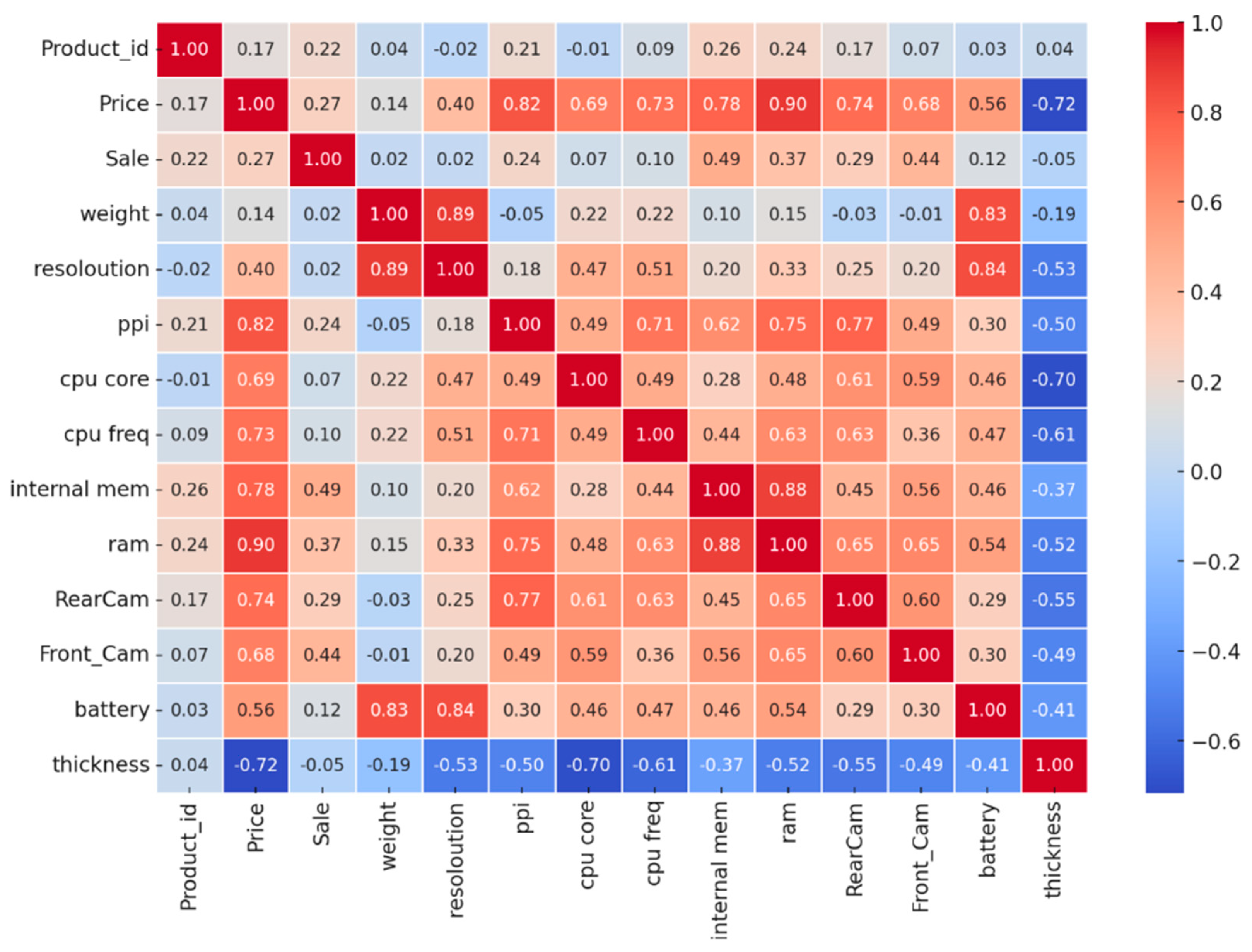
The correlation matrix in Figure 1 reveals relationships between features and price. Internal memory shows a strong positive correlation of 0.84, indicating that more storage capacity is associated with higher prices. RAM also has a significant correlation of 0.80, suggesting that phones with more RAM tend to be priced higher. CPU frequency, with a correlation of 0.78, implies that faster processors contribute to increased pricing. Rear camera quality, at 0.73, is another important factor, showing that better camera specifications lead to higher prices. Battery capacity has a correlation of 0.66, meaning that larger batteries also impact pricing noticeably. Some features exhibit weak or negligible correlations with price. Weight, with a correlation of 0.30, suggests that heavier phones have only a slight influence on price. Thickness, with a correlation of −0.21, indicates that thinner phones tend to be slightly more expensive, though the relationship is weak. There is also a notable negative correlation between sales and price, with a value of −0.64. This suggests that phones with higher sales volumes tend to be lower in price, reinforcing the idea that budget phones are sold in greater quantities than premium models.

The histograms in Figure 2 reveal right-skewed distributions for several features, such as RAM, internal memory, and price, indicating that high-end specifications are less common. Additionally, CPU frequency and RAM display distinct groupings, which result from standard industry configurations. The battery capacity and camera resolution exhibit multiple peaks, corresponding to different product tiers.

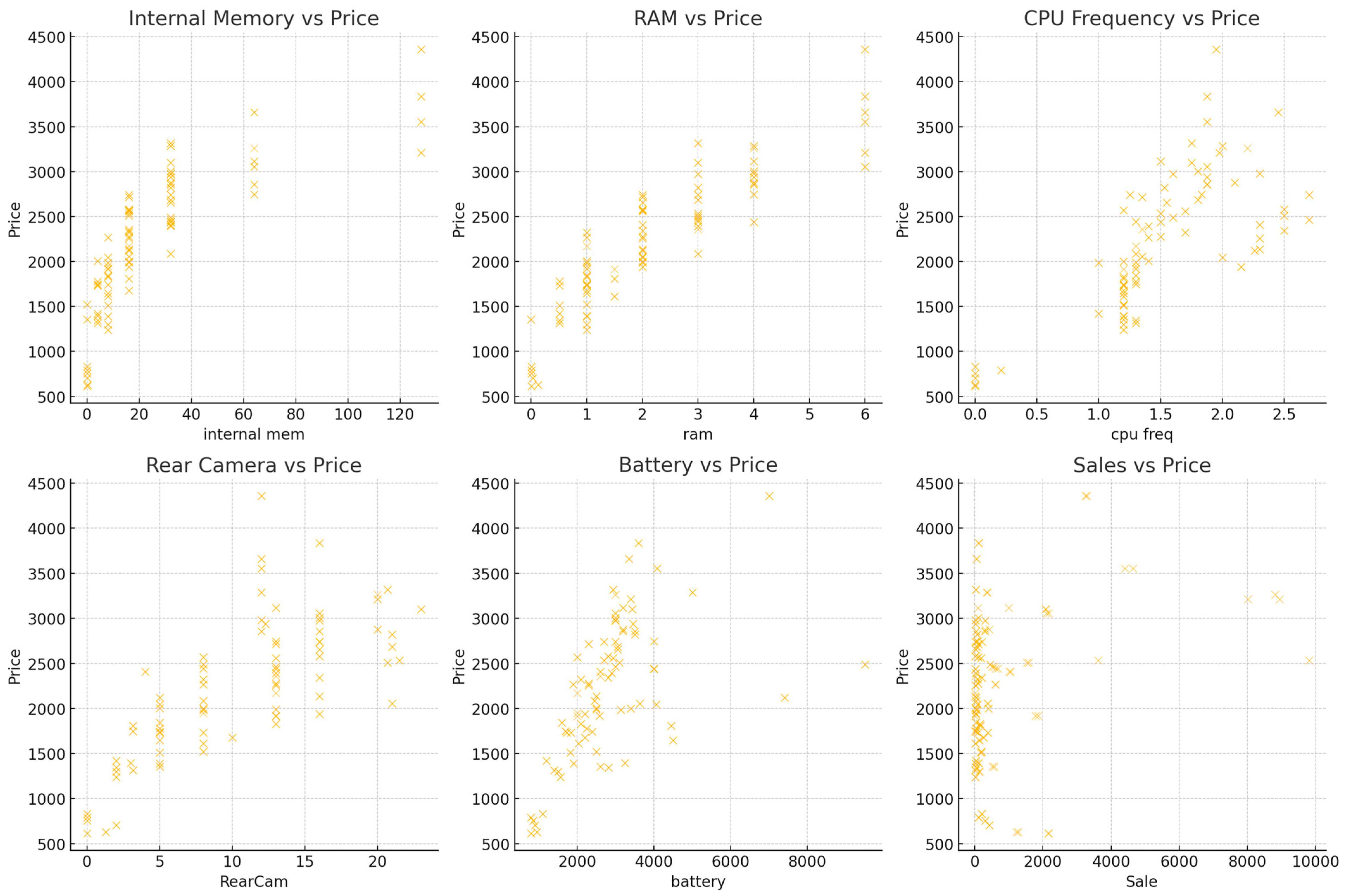
The scatter plots in Figure 3 provide deeper insights into how different features influence price. Internal memory shows a strong positive trend, where price rises significantly as storage capacity increases. Higher storage models, such as 128 GB and above, exhibit a steeper price increase. RAM also demonstrates a strong correlation with price, as higher capacities like 8 GB and 12 GB are associated with more expensive models. The data points are clustered, indicating that common RAM configurations exist in the market. CPU frequency has a moderate positive correlation with price, suggesting that faster processors generally lead to higher prices. However, some variation exists, with certain high-end models featuring lower CPU frequencies yet maintaining premium pricing, due to brand influence. Rear camera quality follows a noticeable positive trend, where higher megapixel counts correspond with more expensive phones. Battery capacity also shows a moderate correlation with price. Larger batteries tend to align with higher-priced models, though the relationship is not as strong as that of RAM or internal storage. Some budget models feature large batteries but remain relatively inexpensive. Increasing RAM, internal memory, and rear camera specifications are the most effective ways to justify a price increase.

4.2. Operational Framework for Implementation

To operationalize the proposed pricing strategy, we present a structured implementation flow in Algorithm 1. This algorithm outlines the steps required to train a regression model, integrate DiCE for counterfactual analysis, and test pricing scenarios through manual and data-driven feature modifications. Each step aligns with typical tasks in corporate pricing workflows, allowing businesses to apply this methodology using existing analytics pipelines and decision support systems. Algorithm 1 further presents the steps of the data-driven price strategy model (ML+DiCE).

Algorithm 1: Operational framework for implementation

1. LOAD AND EXPLORE DATA   a. Load dataset from .csv file.   b. Display dataset information (column names, data types, missing values). 2. PREPROCESS DATA   a. If missing data, handle null.   b. Define features (X) by removing ‘Price’ and ‘Product_id’.   c. Define target variable (y) as ‘Price’.   d. Split data into training (80%) and testing (20%) sets. 3. TRAIN REGRESSION MODEL   a. Initialize Regressor.   b. Train model on (X_train, Y_train).   c. Predict price for test set (X_test).   d. Evaluate performance using R2 score for training and testing, MSE, MAE, MAPE Equations (8)–(11). 4. PREPARE DATA FOR DiCE   a. Add predicted prices to X_test.   b. Define DiCE data object with continuous features.   c. Define DiCE model object based on trained Regressor.   d. Initialize DiCE explainer. 5. GENERATE COUNTERFACTUAL EXPLANATIONS   a. Select a sample mobile phone from X_test (input_record).   b. Compute expected price range (15–20% higher than predicted price).   c. Use DiCE to generate counterfactual feature modifications.   d. Display recommended feature modifications. 6. TEST MANUAL FEATURE MODIFICATIONS   a. Change configuration—modify internal memory (double) and battery capacity (e.g., increase by 50%).   b. Predict new price with modified features.   c. If new price ≥expected minimum price, print “The new configuration meets required price”.   d. Else, print “The new configuration does not meet required price”. 7. TEST MORE AGGRESSIVE MODIFICATIONS   a. Modify internal memory (quadruple), battery (e.g., increase by 50%) and RAM (e.g., double).   b. Predict new price with modified features.   c. If new price >= expected minimum price, print “The new configuration meets required price”.   d. Else, print “The new configuration does not meet required price”. 8. OUTPUT RESULTS   a. Display DiCE-generated recommendations.   b. Display manually tested modifications.   c. Suggest further improvements if necessary (e.g., CPU, display type).

Each step maps to real-world business functions. For example:

Steps 1–3 (Data preparation and model training) align with the tasks of a data science or pricing analytics team;

Steps 4–5 (DiCE integration) provide the decision-making layer where counterfactuals assist product managers or marketers in evaluating pricing scenarios;

Steps 6–7 (What-if testing) allow for manual scenario planning—mirroring how pricing teams might simulate product upgrades in a strategy meeting;

Step 8 (Output results) could feed into internal dashboards, reports, or product development recommendations.

4.3. Simulations

Following the steps in Algorithm 1, the results are summarized in

Table 5. Results of the price prediction.

Metric	R2 Score for Training Data	R2 Score for Inference Data	MSE	MAE	MAPE
	0.993	0.961	18,456.212	108.311	0.0542

. The minimum price in y_test is 754. The maximum price in y_test is 3658. The mean (average) price is around 2000–2500. Since the MSE (18,456.21) is in squared units (as in Table 5), we take the square root to get an idea of the typical error magnitude. This means, on average, our predictions are about 136 units off in squared terms, which aligns with the MAE. Based on MAE (108.31), our model is off by 108.31 units on average. Given that y_test values range from 754 to 3658, an error of approximately 108 units is low relative to the scale of prices. The MAE is a percentage of the mean price (~2500): (108.31/2500) × 100 ≈ 4.33%. This suggests that our model performs well in absolute terms. The MAPE (5.43%) tells us that, on average, our model error is about 5.43% of the actual price. Since the MAPE is less than 10%, this is very good for most applications.

The R² scores indicate how well our model explains the variance in the target variable (y_test). The R² score for the training data is 0.9936 (99.36%), meaning that our model explains 99.36% of the variance in the training data. Such a high R² suggests that the linear regression model fits the training data extremely well, but it also raises concerns about potential overfitting, where the model might be too tailored to the training set. The R² score for the inference (test) data is 0.9615 (96.15%), meaning that our model explains 96.15% of the variance in the test data. This is still very high, indicating that our model generalizes well. The slight drop from the training R² (99.36% to 96.15%) is expected and suggests only minimal overfitting, which is normal. Overall, our linear regression model has excellent performance, with an R² for the test data above 95%, meaning that our predictions are very accurate. The minimal overfitting, with only a small drop from training to test data, confirms that the model generalizes well. When combined with the MAPE value of 5.43%, our model makes low-percentage errors, further supporting its reliability.

The results may even get better without the 10 partially inconsistent records in terms of noise reduction. Inconsistent data (e.g., 0 RAM, 0 CPU cores) introduce unrealistic input–output mappings that confuse the regression model. Excluding them can sharpen the model’s understanding of real-world patterns. The learning may also improve as the model learns from patterns in the data. If 6.21% of the data contain false signals, removing them gives the model a more representative view. With cleaner data, however, the model is less likely to “overfit” on noisy or spurious patterns and might perform better on unseen test data.

The initial configuration of one sample in

Table 6. Predicted price for a certain configuration.

Sale	Weight	Resolution	PPI	CPU Core	CPU freq	Internal Mem	RAM	RearCam
40	169	5.7	515	4	1.875	64	4	12

and

Table 7. Predicted price for a certain configuration.

Front_Cam	Battery	Thickness	Predicted_Price
5	3500	7.9	2948.67

(or the baseline predicted price) consists of a 5.7-inch display, 515 PPI, four CPU cores, 1.875 GHz CPU frequency, 64 GB internal memory, 4 GB RAM, and a 12 MP rear camera, with a 5 MP front camera, a 3500 mAh battery, and a thickness of 7.9 mm. Based on these specifications, the predicted price for this configuration is 2948.67. This baseline price provides a reference point to evaluate how specific modifications impact the product’s market value.

The counterfactual adjustments to increase price by 15–20% are provided in

Table 8. Counterfactual actions to increase the price by 15–20%.

Sale	Weight	Resolution	PPI	CPU Core	CPU Freq	Internal Mem	RAM	RearCam
40	169	5.7	515	4	1.875	64	5.7	12
40	169	5.7	515	4	1.875	64	6.0	12
40	169	5.7	515	4	1.875	64	5.7	12

and

Table 9. Counterfactual actions to increase the price by 15–20%.

Front_Cam	Battery	Thickness	New Price
15.6	3500	7.9	3374.86
5	4877	7.9	3412.45
5	4949	7.9	3503.23

.

To achieve a higher predicted price (15–20% increase), several counterfactual modifications are tested:

• Increasing the front camera resolution from 5 MP to 15.6 MP and RAM from 4 to 5.7 GB, while keeping other specifications constant, raises the predicted price to 3374.86, showing that a better front camera contributes significantly to perceived value.
• Increasing the battery capacity from 3500 mAh to 4877 mAh and RAM from 4 to 6 GB results in a price increase to 3412.45, suggesting that larger battery capacity is another key driver of price improvement.
• Further increasing the battery to 4949 mAh and RAM from 4 to 5.7 GB leads to the highest new price of 3503.23, confirming that extended battery is an essential factor in pricing decisions.

The analysis reveals that front camera resolution and battery capacity are the most influential features in increasing the predicted price. Upgrading the front camera to 15.6 MP provides a notable boost in price, while improving battery capacity beyond 4877 mAh results in even higher pricing. Interestingly, RAM modifications (from 4 GB to 5.7 GB and 6.0 GB) appear to have a minimal effect on price predictions, indicating that RAM upgrades alone may not significantly increase a mobile phone’s market value. If the goal is to achieve a p = 15–20% price increase, manufacturers should focus on enhancing the front camera and battery capacity, as these features contribute the most to perceived product value.

The results in

Table 10. What-if analysis to attain the goal by different means.

Configuration	Expected Internal Memory	Expected Battery	Expected RAM	New Price	Meets Minimum Expected Price (3350.0)
Config 1	2 × Internal Memory	1.5 × Battery	—	3226.13	No
Config 2	4 × Internal Memory	1.5 × Battery	1.5 × RAM	3649.42	Yes

indicate how modifying specific product features affects the predicted price and whether the minimum expected price of 3350.0 is achieved. In the first configuration, doubling the internal memory and increasing the battery capacity by 1.5 times results in a predicted price of 3226.13. However, this configuration does not meet the minimum expected price threshold. In contrast, the second configuration applies more significant feature enhancements by quadrupling the internal memory, increasing the battery by 1.5 times, and expanding the RAM by 1.5 times. These modifications lead to a higher predicted price of 3649.42, successfully exceeding the minimum expected price of 3350.0. The results suggest that moderate improvements in internal memory and battery alone are insufficient to achieve the desired price increase. However, a more substantial enhancement, particularly by increasing internal memory significantly and improving RAM alongside battery capacity, effectively raises the product’s perceived value and predicted price. Table 10 summarizes other configurations and their outcomes.

Table 10 provides a clear comparison of how different adjustments to product features impact the predicted price and whether the desired pricing threshold is met.

5. Discussion

This section links our research to corporate finance theory and provides a discussion of AI methodologies, including the rationale for using DiCE and limitations. In corporate finance, product pricing decisions are closely tied to theories of value creation, profitability maximization, and strategic investment in product differentiation [48,49]. Theories such as the shareholder value maximization model emphasize the importance of aligning product attributes with consumer willingness to pay in order to enhance firm value [50]. Additionally, value-based pricing strategies [51], rooted in microeconomic pricing theory, advocate setting prices based on the perceived or estimated value that a product delivers to the customer rather than solely on cost-plus or competition-based pricing.

Our research aligns with these principles by using a data-driven model to identify product attributes that contribute most significantly to price increases. The proposed methodology can support corporate decisions about resource allocation for product development [52], as it quantifies the potential return (in terms of pricing power) of enhancing specific features.

Artificial intelligence (AI) has increasingly been adopted in pricing models across industries, offering several benefits. ML algorithms, particularly tree-based models (e.g., random forests and gradient boosting), have shown high predictive accuracy and the ability to capture nonlinear relationships between features and price. However, these models often lack transparency, making it difficult for businesses to justify or interpret price recommendations, an essential issue in corporate decision making and communication with stakeholders. In contrast, explainable AI (XAI) techniques [53], including counterfactual explanations, provide insights into why a particular decision or prediction was made. This transparency is valuable in corporate finance settings where the auditability, interpretability, and traceability of decisions are required for strategic and regulatory reasons. The use of DiCE in our research is grounded in the need for both predictive power and interpretability. DiCE reveals how feature modifications (e.g., increasing battery capacity or front camera resolution) can influence that price. This aligns with corporate pricing strategies that seek to evaluate trade-offs between feature improvements and their market impact. The benefits of using DiCE in our context include the following: (a) identifying specific, minimal changes needed to reach a desired price point; (b) offering intuitive “what-if” scenarios, aiding decision makers in understanding model behavior; and (c) bridging the gap between black-box models and stakeholder trust. By integrating DiCE into a structured pricing framework, our research contributes to the field of explainable, data-driven pricing strategies. It extends existing research by applying XAI not to customer behavior prediction or segmentation, but directly to product-level pricing decisions, offering both methodological novelty and managerial relevance.

However, we also acknowledge limitations. DiCE assumes a stable underlying predictive model, and the quality of its explanations depends on the correctness and generalizability of the regression function used. Additionally, counterfactuals are sensitive to the input space and may not always reflect practical or feasible modifications from a product development standpoint.

6. Conclusions

The proposed data-driven pricing strategy model integrates machine learning with counterfactual analysis to optimize product pricing. The model was developed using a structured process that involved data exploration, preprocessing, training a regression model (linear regression), and applying DiCE for counterfactual explanations. The performance evaluation demonstrated that the linear regression model predicts prices with high accuracy, achieving an R² score of 96.15% for test data while maintaining minimal overfitting. The model’s error metrics, including an MAE of 108.31 and a MAPE of 5.43%, indicate strong predictive capabilities relative to the price range.

Through counterfactual analysis, we examined which feature modifications could increase a mobile phone’s predicted price by 15–20%. The analysis revealed that upgrading the front camera resolution and increasing battery capacity were the most influential changes in achieving a higher predicted price. While increasing RAM contributed to pricing improvements, its impact was less significant than enhancements to the front camera and battery. The results suggest that manufacturers seeking to optimize smartphone pricing should prioritize these attributes.

The “what-if” analysis confirmed that moderate improvements, such as doubling internal memory and slightly increasing battery capacity, were insufficient to meet the desired price increase. However, more aggressive modifications, including quadrupling internal memory and increasing battery and RAM capacity by 1.5 times, successfully raised the predicted price above the minimum expected threshold. The comparative evaluation further illustrates how different configurations impact pricing outcomes.

Our research demonstrates the effectiveness of combining machine learning (linear regression) with counterfactual explanations (DiCE) for pricing optimization. The proposed approach enhances transparency in pricing decisions, allowing businesses to justify price points while dynamically adjusting to market conditions.

Returning to the RQs exposed in the Section 1, the following direct answers are provided:

RQ1: Can machine learning models accurately predict smartphone prices based on technical specifications? The results confirm that machine learning models can predict smartphone prices with high accuracy using only technical specifications. The model achieved an R² score of 96.15% on test data and a MAPE of 5.43%, indicating strong predictive performance and minimal error relative to the overall price range.

RQ2: Which features contribute most significantly to price increases? In our analysis, we identified internal memory, RAM, CPU frequency and rear camera resolution as having the strongest positive correlations with price. However, the counterfactual simulations showed that internal memory and battery capacity were the most impactful for achieving target price increases, especially when aiming for a 15–20% increase. This means that while some features correlate strongly with price, others are more influential when it comes to actionable price optimization.

RQ3: How can counterfactual explanations be used to support actionable, business-oriented pricing strategies? Counterfactual explanations generated using DiCE effectively identified the minimal and targeted feature modifications required to reach a higher price point. These explanations provided actionable insights, such as increasing the battery capacity, which product managers or marketing teams may use to guide feature development and pricing decisions.

One limitation of the study is the lack of detailed information regarding the provenance of the dataset. Apart from knowing that the dataset was uploaded or last updated three years ago, the authors do not have access to further contextual details, such as the data collection period, the sources involved, or the criteria used in assembling the data. However, since the dataset is open source and was not created by the authors, this limitation is beyond their control and could not be addressed or influenced within the scope of this work. Another limitation is that it focuses exclusively on mobile phones and relies on a dataset that includes only technical specifications, without incorporating other influential factors, such as brand perception, marketing strategies, or consumer preferences. As a result, the model may overemphasize the role of hardware components in determining price, potentially overlooking the broader and more complex drivers of product valuation.

As part of future work, we intend to expand the scope of our analysis by incorporating additional product categories beyond mobile phones, particularly those in which non-technical factors, such as brand value, marketing influence, and consumer perception, play a significant role in pricing.