Abstract
With the continuous upgrading of consumer demand and retail modes, more and more retailers are switching to an omnichannel retail mode. In order to study the location problem of offline physical stores of online retail enterprises that plan to implement the BOPS (Buy Online and Pickup in Store) omnichannel retail model, this paper considers consumers’ choice behavior under the omnichannel retail model; uses the MNL (Multinomial Logit) model to depict customers’ choice behavior between the online channel, BOPS channel, and offline physical channel; and constructs a location optimization model of offline physical stores with the goal of minimizing the enterprise’s cost. According to the characteristics of the model, an improved genetic algorithm was designed; the algorithm was improved on chromosome selection mode, crossover, and mutation rules. Finally, an example is calculated, and the physical store location scheme of a retail enterprise and the vehicle routing optimization scheme under the two-level distribution network are obtained, which verifies the effectiveness of the model and algorithm and provides a scientific reference for the physical store location decision of online retail enterprises planning to implement the BOPS omnichannel retail model. The impact of freight, return rate, and service level of physical stores on the location of offline physical stores is analyzed. The results show that in the process of expanding offline physical stores to implement the BOPS omnichannel retail model, online retail enterprises can reduce enterprise costs by improving the freight level and service level of the physical store. The higher the return rate of the online channel, the more necessary it is to expand offline physical stores, and the lower the enterprise cost. At the same time, management suggestions are put forward for the enterprise operation under the BOPS omnichannel retail mode.
1. Introduction
“New retail” is a new consumption model born from technological innovation and consumption upgrading. It takes consumers as the center and uses big data technology to organically integrate online, offline, and logistics to better meet the diversified needs of consumers. With the continuous improvement of people’s living standards, the retail industry has come into the customer-centered era [1]. Customers can purchase products through online channels, physical channels, and BOPS (Buy Online and Pickup in Store) channels [2]. If retailers want to seek long-term development, they must meet customers’ multi-channel purchase needs. Especially for traditional online retailers, the user growth and traffic dividend brought by the popularity of the internet are gradually shrinking, and online retail is facing a growth bottleneck. Customers pay more and more attention to product quality and shopping experience [3]. Online retailers may deliver products that fail to meet customers’ expectations, leading to return [4], and their after-sales service quality is also a key factor affecting customer satisfaction [5]. In addition, customers’ demand for personalized services keeps increasing [6]. Online retailers cannot communicate with customers face-to-face about products, and lack of humanized services affects customers’ shopping experience. Customers also have higher requirements on the delivery cycle of online retailers [7]. If the online retailer fails to deliver the product within the time the customer expects, it will create a poor shopping experience for the customer and lead to the return of the product. At the same time, the short expectation time also encourages customers to purchase products through the physical channel or the BOPS channel. This has prompted online retailers to transform into a new retail model of BOPS omnichannel.
Omnichannel operations can improve retailers’ earnings [2] and maintain good competitive advantages [8]. After online retailers implement the BOPS omnichannel retail model, the physical channel can provide consumers with visibility, tangibility, audibility, and other physical shopping experiences, making up for the deficiency of the online channel. The BOPS channel can meet consumers’ consumption demand for comprehensive channels and improve their consumption experience. In recent years, more and more retail enterprises have opened the BOPS omnichannel retail mode for consumers, which has a significant impact on online and offline sales and consumption flow [9]. For example, the new retail fresh food chain supermarket represented by Alibaba’s “Hema Fresh”, with the support of big data, cloud computing, and other technologies, has laid out an omnichannel retail model, optimized the store layout and distribution network, and promoted the retail upgrading of the fresh food industry. The location of offline physical stores is one of the key issues for online retailers to expand the BOPS omnichannel retail model. Choosing a reasonable location for physical stores is helpful to control enterprise costs and improve their service level [10]. Under the BOPS omnichannel retail model, physical store location and network distribution are a cooperative system, which jointly build the whole omnichannel sales and bring a higher quality shopping experience to consumers. On the one hand, physical stores can provide customers with real shopping scenes, provide a good shopping experience [11], and meet customers’ demands for a physical channel and a BOPS channel. On the other hand, physical stores have the function of a pre-warehouse, optimize the distribution network of new retail enterprises, shorten the delivery and distribution cycle of the online channel, and enhance customers’ experience of the online channel. The location of physical stores in China has various forms and fast transformation speed, which can be used as a combination of operational and strategic decisions, including independent investment, acquisition of existing physical stores, and other forms.
Through the review of the literature on offline physical store location, the relevant research rarely considers the consumer’s choice behavior. Under the omnichannel retail model, consumers can choose different channels to purchase products [12], and new retail enterprises attach great importance to consumers’ shopping experience. Obviously, it is inappropriate to ignore consumer behavior factors when studying offline physical store location under the BOPS omnichannel retail model. It is important to explore consumer choice behavior under the three purchase channels.
Motivated by this observation, this paper aims to understand the location problem of offline physical stores of online retail enterprises that plan to implement the BOPS omnichannel retail model, considers consumer behavior factors under the omnichannel retail environment, depicts customers’ choice behavior of the online channel, BOPS channel, and offline physical channel when purchasing products, and constructs an offline physical store location optimization model with the goal of minimizing the total cost of the enterprise. It is expected to provide scientific reference for the offline physical store location and distribution route optimization decision of online retail enterprises that plan to implement the BOPS omnichannel retail model.
The rest of this paper is organized as follows. Section 2 reviews the relevant literature. Section 3 describes relevant research methods, including characterization of consumer behavior, location model, and heuristic algorithm. In Section 4, numerical and example analysis is carried out, and the results of this paper are obtained and discussed. Section 5 puts forward conclusions.
2. Literature Review
This paper studies the location problem of offline physical stores under the new retail model and considers the impact of consumers’ choice behavior on the location decision. Therefore, the literature search mainly focuses on three research streams: new retail model, physical store location, and consumer choice behavior.
2.1. New Retail Model
For the new retail model of online and offline integration, scholars have proved the effectiveness of BOPS omnichannel operation through relevant research. Fan et al. [13] proposed that the BOPS channel attracts existing and potential customers and found that the BOPS channel should be introduced when the service level of all channels is low. Song et al. [2] analyzed the effectiveness of an omnichannel operation by comparing the balanced profit and consumer surplus of the online channel, physical channel, and BOPS channel. Some scholars have studied cross-channel returns, pricing, inventory strategy, and other issues under an omnichannel operation. Radhi and Zhang [14] considered cross-channel return and explored the influence of re-sold returned products on the quantity of orders in each channel. Pichka et al. [15] studied the pricing and fulfillment decisions of omnichannel retailers. Paul et al. [16] studied the inventory replenishment problem in physical stores when consumers purchase online and pick up the purchased goods in physical stores. Bayram et al. [17] considered a new retail enterprise with an online channel and a physical channel, and studied the fulfillment of customer orders with the goal of maximizing the retailer’s overall profit. For the location problem, Huang et al. [10] studied front distribution center location under an omnichannel retailing model by considering such factors as facility capacity, demand, and rent fluctuation. There is little research on offline physical store location under the BOPS omnichannel model. This paper further studies offline physical store location by considering consumer choice behavior.
2.2. Physical Store Location
Scholars have done a lot of research on the location of physical stores and distribution centers of retail enterprises. Some studies focused on the time demand of customers. Wang et al. [18] focused on the time requirements of customers and constructed a vehicle path optimization model of cold chain logistics considering the time window. Wang et al. [19] studied the two-level location path problem with time window considering customer clustering. Dou et al. [20] introduced constraints such as freshness and time window and established a location optimization model for a cold chain logistics distribution center. Carbon emissions have also attracted the attention of scholars. Zhang et al. [21] constructed a location model of a cold chain logistics distribution center based on a two-level programming method considering carbon emissions. Li et al. [22] established a multi-objective location model for a cold chain logistics distribution center considering carbon emissions. Alamatsaz et al. [23] studied the low-carbon location-routing problem by considering time window and carbon emissions at the same time. In addition, scholars have also carried out relevant research on location differences, decision-making methods, uncertain demands, and other aspects. Ouyang et al. [24] improved the location of retail stores by considering the spatial distribution differences of location factors. Agrebi and Abed [25] used the improved multi-attribute, multi-actor decision-making method to solve the distribution center location problem in an uncertain environment. Fathi et al. [26] developed a two-phase approach based on queuing theory and stochastic optimization to determine the optimal number and location of distribution centers. Liu et al. [27] studied the three-level optimal location problem under the condition of uncertain transportation cost and customer demand. Marianov et al. [28] studied the location of retail stores considering customers’ purchase of multiple commodities. Zhang et al. [29] first used the distance between township logistics nodes to conduct AP clustering, and then constructed an optimization model for an agricultural product joint distribution center. Yu et al. [30] studied the two-echelon vehicle routing problem with time windows, covering options, and occasional drivers. The above studies have studied the location of physical stores or distribution centers of retail enterprises with different emphases, and obtained reasonable location schemes for physical stores or distribution centers. However, all the above studies assume that customers are completely rational. In fact, customers have the option of choosing from various purchase channels, and ignoring customer behavior factors in the process of planning location will lead to a decrease in customer consumption experience.
2.3. Consumer Choice Behavior
For research on consumer behavior under the new retail model, Yang et al. [31] studied consumer behavior and psychology considering mileage anxiety and loss anxiety. Xu and Jackson [32] examined the influential factors of customer channel selection intention in an omnichannel retail setting and found that channel transparency, channel convenience, and channel uniformity positively influenced customer perceived behavioral control. The MNL model is a common method used by scholars to depict consumer choice behavior. Marianov et al. [33] applied the MNL model to the facility location model considering facility congestion. Zhang et al. [34] established a network design model of preventive medical facilities by using the MNL model, considering customers’ participation in preventive rescue programs. Haase and Mueller [35] used the MNL model to depict customers’ choice behavior and incorporated customers’ choice into the location planning of preventive health facilities. Al-Salih and Esztergár-Kiss [36] used the MNL model to describe residents’ travel mode choice. The MNL model is also used to describe consumers’ choice of cancer detection facilities [37,38]. It can be seen that the MNL model is an effective method for depicting consumer behavior, but it has not been applied to the research on consumer choice behavior under the BOPS omnichannel retail model. Therefore, this paper uses the MNL model to study consumer choice behavior in the offline physical store location problem under the BOPS omnichannel retail model.
2.4. Summary
We summarize the literature related to the location problem according to the study focus, customer behavior, behavior description mode, and solution approach in Table 1.

Table 1.
Literature comparison.
To sum up, few papers on the location of physical stores or distribution centers consider customer choice behavior, and only a few papers on the location of preventive medical facilities consider customer choice behavior. One of the key problems for online retail enterprises in implementing the BOPS omnichannel model is the construction of offline physical stores, and consumer behavior is also an important factor to be considered. As can be seen from the above literature, the MNL model is a common method used to describe customer choice behavior. In addition, heuristic algorithms are often designed to solve the location model. Therefore, in view of the problem of consumer behavior not being taken into account in previous literature on physical store location, the MNL model is used to describe consumers’ choice among three purchase channels. We construct a location optimization model of offline physical stores under the BOPS omnichannel retail model with the goal of minimizing the total cost and design and create an improved genetic algorithm to solve the model.
3. Methods
3.1. Problem Description and Conditional Assumptions
3.1.1. Problem Description
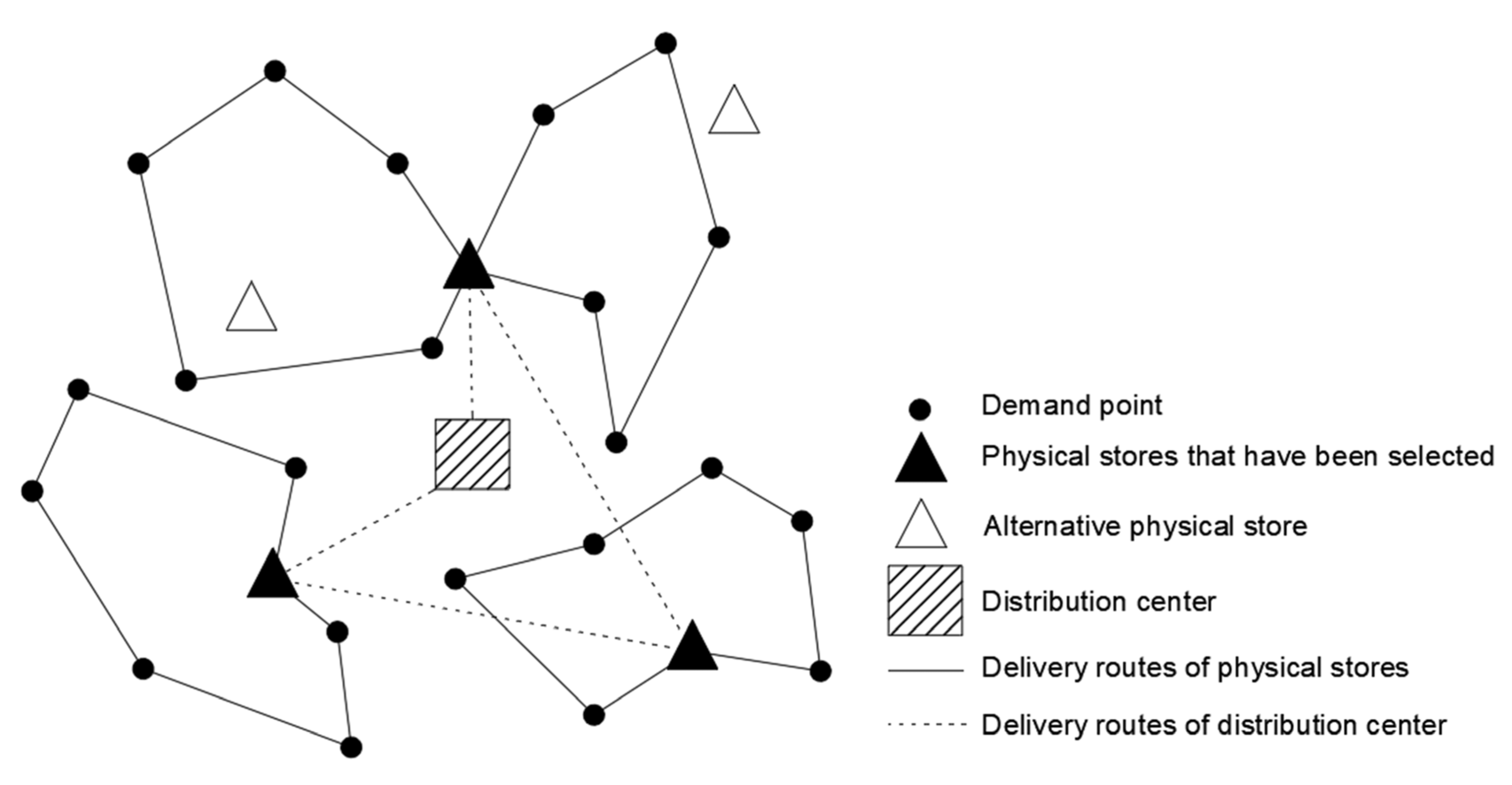
This paper considers the online retail enterprise that plans to implement the BOPS omnichannel retail model. According to the previous relevant statistical data, it divides all customers in the distribution area of a distribution center into several demand points. Based on different customer choice behaviors with regard to demand points, it constructs an offline physical store location model with the minimum total cost and optimizes the distribution route. Offline physical stores, together with distribution centers and demand points, form a two-level distribution logistics network while meeting customers’ demands in the offline physical channel and BOPS channel, as shown in Figure 1.
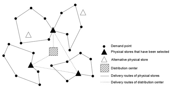
Figure 1.
Schematic diagram of logistics system.
3.1.2. Conditional Assumptions
For the convenience of research, the following assumptions are made in this paper, and the model parameters and variables are shown in Table 2.

Table 2.
Model parameters and decision variables.
- (1)
- The total demand of each demand point is known, and only a single product is considered.
- (2)
- The locations of each demand point and alternative physical stores are known.
- (3)
- The number of physical stores required to be built is limited, and the construction cost of physical stores is the same.
- (4)
- Regardless of the inventory level of physical stores, all physical stores balance supply and demand.
- (5)
- The demand of physical stores is met by the distribution center. Customers’ demands in the physical channel, online channel, and BOPS channel are met by physical stores.
- (6)
- The online channel needs of customers in each demand point can only be met by one physical store. One physical store can meet the online channel needs of customers in multiple demand points, and goods cannot be transferred between physical stores.
- (7)
- From the distribution center to the physical store and from the physical store to the demand point, two kinds of vehicles with different load capacities are used for distribution. The number of vehicles owned by the enterprise is known.
- (8)
- The delivery vehicle must return to the original place of departure after completing the delivery task. The traffic speed is constant, and the road is clear.
- (9)
- There is no product shortage problem in any channel.
3.2. Characterization of Customer Choice Behavior
The MNL model is an important method for describing customer choice behavior [39]. According to the random utility theory, consumers choose a purchase channel according to the utility provided by each channel under the BOPS omnichannel retail environment [12]. This paper constructs the utility function of each purchase channel and uses the MNL model to characterize consumer choice behavior.
3.2.1. Utility Function
With the development of online and offline integration in the retail industry, customers can purchase products through an online channel, physical channel, and BOPS channel [2]. The utility obtained by customers from different channels is different.
- (1)
- Online channel utility function
If customers choose the online channel, they need to pay a fixed freight [40]. Referring to the research on the impact of freight on customer utility in literature [40], this paper assumes that the acceptable freight interval for customers is . When ≤, the utility of freight on customers is 1. When ≥, is 0. In between, decreases as increases. In order to facilitate calculation, the following linear decreasing function is used to describe the utility of freight to the customer.
After customers purchase products through the online channel, they may be dissatisfied with the delivered products and return them. In the actual situation, enterprises can calculate the average return rate of each demand point according to previous data. For the convenience of this study, it is assumed that the average return rate of each demand point follows a uniform distribution. Therefore, considering the return and freight borne by customers, the utility function of customers choosing the online channel to purchase products is
- (2)
- BOPS channel utility function
In the process of customers picking up products, pickup distance is the key variable affecting customers’ utility. Customers tend to choose whether to pick up their products in physical stores according to the pickup distance and often choose the physical store with the shortest distance. Therefore, this paper assumes that the pickup distance of customers purchasing products through the BOPS channel is the shortest distance between customers and all physical stores, assuming that the maximum pickup distance accepted by customers is and the minimum pickup distance expected by customers is . Based on the gradual covering theory, the concave and convex covering function is used to describe the utility function of the customer’s pickup distance:
where
is the pickup distance at demand point and is the distance sensitivity coefficient of customers, which varies from customer to customer in the actual situation. For the convenience of research, it is assumed that the distance sensitivity coefficient of all customers is the same.
When customers go to a physical store to pick up their own products, the service level of physical store will also have an impact on customer utility. The service level of physical stores is related to communication convenience, quick delivery process, and other factors. In the actual situation, enterprises can evaluate the service level of each physical store according to these factors. For the convenience of calculation, we refer to the description of the attractiveness of different shelters to residents in the literature [41] and assume that the service level of a physical store follows a uniform distribution. Therefore, considering the pickup distance and service level of a physical store, the utility function of customers choosing the BOPS channel to purchase products is
- (3)
- Offline physical channel utility function
When customers choose the offline physical channel to purchase products, the distance to a physical store is the same as the pickup distance when they choose the BOPS channel. In addition, customers who choose the offline physical channel often want to perceive and experience the products before purchasing. The more shopping time they have, the more they can fully perceive and experience the products. The more consumers know about product information, the more they can buy products that satisfy them. Customers can estimate their own shopping time before choosing the purchase channel, assuming that the shopping time of customers at each demand point is uniformly distributed.
Referring to the description of the impact of pickup time on customer utility in the literature [40], it is assumed that the shortest shopping time accepted by customers is and the expected shopping time is . The utility function of customers’ shopping time is expressed by a linear increasing function:
Therefore, considering the distance to a physical store and shopping time, the utility function of customers choosing the offline physical channel to purchase products is:
where represents the utility weight of the customer’s distance to the physical store, which can be obtained through expert investigation.
3.2.2. Customer Channel Choice Behavior
The MNL model is adopted to describe customers’ choice among three purchase channels. The probability of customers at demand point choosing the online channel to purchase products is:
The probability of customers at demand point choosing the BOPS channel to purchase products is:
The probability of customers at demand point choosing the offline physical channel to purchase products is:
3.3. Model Construction
This paper mainly considers the construction cost of offline physical stores, vehicle transportation cost, and penalty cost caused by customer returns, and constructs a location optimization model.
3.3.1. Construction Cost of Offline Physical Stores
Assuming that the size and area of physical stores are exactly the same, construction cost of offline physical stores is:
3.3.2. Vehicle Transportation Cost
Small delivery vehicles are used to deliver products from physical stores to demand points, and delivery distance from physical store to demand point is the driving distance of a vehicle from the physical store to the demand point :
Transportation cost of small delivery vehicles is equal to the sum of the product of delivery distance and delivery quantity of each demand point:
The quantity of goods purchased by customers through the online channel and delivered by offline physical stores can be expressed as:
The quantity of goods purchased by customers through the BOPS channel and picked up at physical stores can be expressed as:
where
The quantity of goods purchased by customers through offline physical channel can be expressed as:
Therefore, the total demand of physical store is:
Delivery distance from distribution center to physical store is the driving distance of a vehicle from the distribution center to the physical store :
Transportation cost of large delivery vehicles is equal to the sum of the product of delivery distance and delivery quantity of each physical store:
Therefore, the total cost of vehicle transportation is:
3.3.3. Penalty Cost of Return
When customers are not satisfied with the products purchased online, they will return the products, and the enterprise needs to bear the processing cost of the returned products. Therefore, the penalty cost of return generated by unsatisfied customer demand is established as:
3.3.4. Objective Function
Based on the above analysis, an offline physical store location optimization model considering customer choice behavior can be built as follows:
s.t.
The objective (23) represents the minimum total cost of the enterprise. Constraint (24) indicates the limitation in the number of physical stores. Constraint (25) indicates that there must be a vehicle driving out of the physical store. Constraint (26) ensures that if a vehicle enters a node, it also exits from the node. Formula (27) indicates that vehicle can only drive out of the physical store that has been built. Constraints (28) and (29) eliminate sub-cycles between customers and physical stores. Constraint (30) ensures that each vehicle can only start from one physical store at most. Constraint (31) ensures that each customer has only one vehicle to serve it. Constraint (32) indicates that vehicle cannot drive between physical stores. Constraint (33) indicates that vehicle will return to the original physical store after delivery. Constraints (34) and (35) represent the carrying capacity constraint of vehicles and . Constraint (36) ensures that if vehicle enters a node, it also exits from the node. Constraint (37) ensures that each physical store has only one vehicle to serve it. Constraint (38) indicates that vehicle returns to the distribution center after delivery. Constraints (39)–(42) represent a value range of the decision variable.
3.4. Design of Improved Genetic Algorithm
In view of the complexity of the variable relationship in the offline physical store location optimization model based on the MNL model constructed in this paper, it is necessary to design an algorithm according to the characteristics of the problem. The genetic algorithm is widely used in studying the location problem. As a global optimization algorithm with good stability, it has the characteristics of simple processing, fast solution speed, and strong scalability. Based on the characteristics of the problem, this paper improves the genetic algorithm in terms of chromosome selection mode and the selection of crossover and mutation probability in order to solve the problem that traditional genetic algorithms are prone to fall into of local optimization and prematurity.
3.4.1. Chromosome Coding and Initial Population Formation
The coding structure of the chromosomes is shown in Table 3. Each chromosome consists of five gene fragments. Gene fragment A has digit, which randomly generates natural numbers from 1 to , representing the matching relationship between demand points and small delivery vehicles. and are the total number of demand points and the number of small delivery vehicles, respectively. Gene fragment B also has digit, which is a random number arrangement from 1 to , representing the service order of demand points. Gene fragment C has digit. It randomly generates natural numbers from 1 to , where the number of genes that are not duplicated is less than or equal to , representing the corresponding relationship between small delivery vehicles and alternative physical stores. is the number of alternative locations of physical stores, and is the limitation in the number of physical stores. Gene fragment D has digit, which randomly generates natural numbers from 1 to , representing the assignment relationship between physical stores and large delivery vehicles. is the number of large delivery vehicles from the distribution center to physical stores. Gene fragment E also has digit, which is a random number arrangement from 1 to , representing the service order of physical stores. Set the population size, and then randomly generate individuals in the population according to the coding rules.

Table 3.
Chromosome coding design.
Assuming = 4, = 3, = 2, = 1, = 2, a randomly generated chromosome is shown in Figure 2. This chromosome indicates that: the physical store location scheme is physical store 1 and 2; the distribution route of small delivery vehicle 1 is physical store 2→demand point 4→demand point 1→physical store 2; the distribution route of small delivery vehicle 2 is physical store 1→demand point 2→demand point 3→physical store 1; and the distribution route of large delivery vehicle 1 is distribution center→physical store 2→physical store 1→distribution center.

Figure 2.
Schematic diagram of chromosomal genes.
3.4.2. Calculation of Individual Fitness
This paper aims to minimize the total cost of the enterprise, and the fitness function is the reciprocal of the objective function.
3.4.3. Selection
Elite retention strategy is introduced to improve roulette strategy to solve the problem that individuals with high fitness occupy the population rapidly in the early stage and the population stops evolving in the later stage due to the small difference in fitness of individuals in the population.
First, the individuals in the population are sorted according to the level of fitness from high to low, and then the first third of the individuals are duplicated twice, the middle third of the individuals are duplicated once, and the rest are eliminated. We get the parent population.
3.4.4. Crossover
In this paper, an adaptive mechanism is introduced to dynamically adjust the traditional fixed crossover probability, which is conducive to generating high-quality solutions and avoiding damaging the good chromosome structure. The calculation formula for crossover probability is as follows:
where is the highest fitness in the population, is the mean of fitness in the population, is the greater fitness of two crossover individuals, and are constant, and .
Crossover individuals are selected with the crossover probability . Crossover location is randomly selected. The two-point crossover method is adopted for gene fragments A and D, and the partial mapping crossover method is adopted for gene fragments B, C, and E. New individuals are created in the above way.
3.4.5. Variation
In order to break local optimum and avoid destroying good structure, dynamic variation probability is adopted in this paper to improve the traditional variation probability. The calculation formula for variation probability is as follows:
where and are the minimum and maximum value of variation probability, respectively, is the continuous generation with no change in highest fitness, and is the largest continuous generation with no change in highest fitness. In this way, when the local optimum occurs, the local optimum can be jumped out by variation, and when the population evolves normally, it can avoid destroying good individual structure with low variation probability and assist in a crossover operation to carry out population evolution.
The chromosomal variation location is determined randomly. The two-point variation method is adopted for gene fragments A and D, and reverse order variation method is adopted for gene fragments B, C, and E. By comparing the performance of a variant chromosome with that of its parent, the individual with excellent performance is retained.
3.4.6. Algorithm Termination
The maximum number of iterations of the algorithm is set. If the optimal solution is not improved after the maximum number of iterations, the algorithm will terminate, and the individual with the maximum fitness will be output.
4. Example Results and Discussion
4.1. Example Verification
According to the survey, an online retail enterprise that plans to implement the BOPS omnichannel retail model needs to establish offline physical stores in a certain area to meet customers’ purchase needs in the physical channel and BOPS channel, improve customers’ consumption experience, and shorten the delivery cycle when customers purchase products through the online channel. For the consideration of trade confidentiality, we have processed the following data. The enterprise divides the consumers in this area into 30 demand points according to the previous relevant statistical data, and the relevant information of demand points is shown in Table 4. Through an investigation into land price, transportation, and market demand distribution in the region, the enterprise has selected 10 alternative physical store addresses. Combined with the enterprise’s own operating conditions, it decides to select no more than six locations among the alternative physical store addresses to build physical stores. Construction cost of a physical store is CNY 20,000. Information about the alternative physical stores is shown in Table 5. The relevant information about the distribution center of the enterprise in this region is shown in Table 6. Two large delivery vehicles and six small delivery vehicles can be assigned to this region. The carrying capacity of large delivery vehicles is 1200 kg, and the unit distribution cost is CNY 30/kg⋅km. The carrying capacity of small delivery vehicles is 200 kg, and the unit distribution cost is CNY 15/kg⋅km. In addition, according to the statistics of the related processing cost of returned products, the unit penalty cost of returned products is set as CNY 5/kg.

Table 4.
Demand point information.

Table 5.
Alternate physical store information.

Table 6.
Distribution center information.
Through the investigation and research on customer behavior in the region, the enterprise ascertains that the acceptable freight interval for customers is [CNY 5, CNY 10]. The average return rate of demand points follows U (0.1, 0.3). The enterprise sets the freight for customers who choose to purchase products through the online channel as CNY 8. When customers choose the offline physical channel or the BOPS channel to purchase products, the acceptable distance interval is [10 km, 40 km], and the distance sensitivity coefficient of consumers is set as 1. The average shopping time of customers of each demand point in the physical store follows U (0.1, 1.2). The expected shopping time is 1 h, and the shortest shopping time accepted by customers is 0.2 h. In addition, the service level of physical stores follows U (0.6, 0.8). When a customer chooses the offline physical channel, the utility weight of the customer’s distance to a physical store is 0.5.
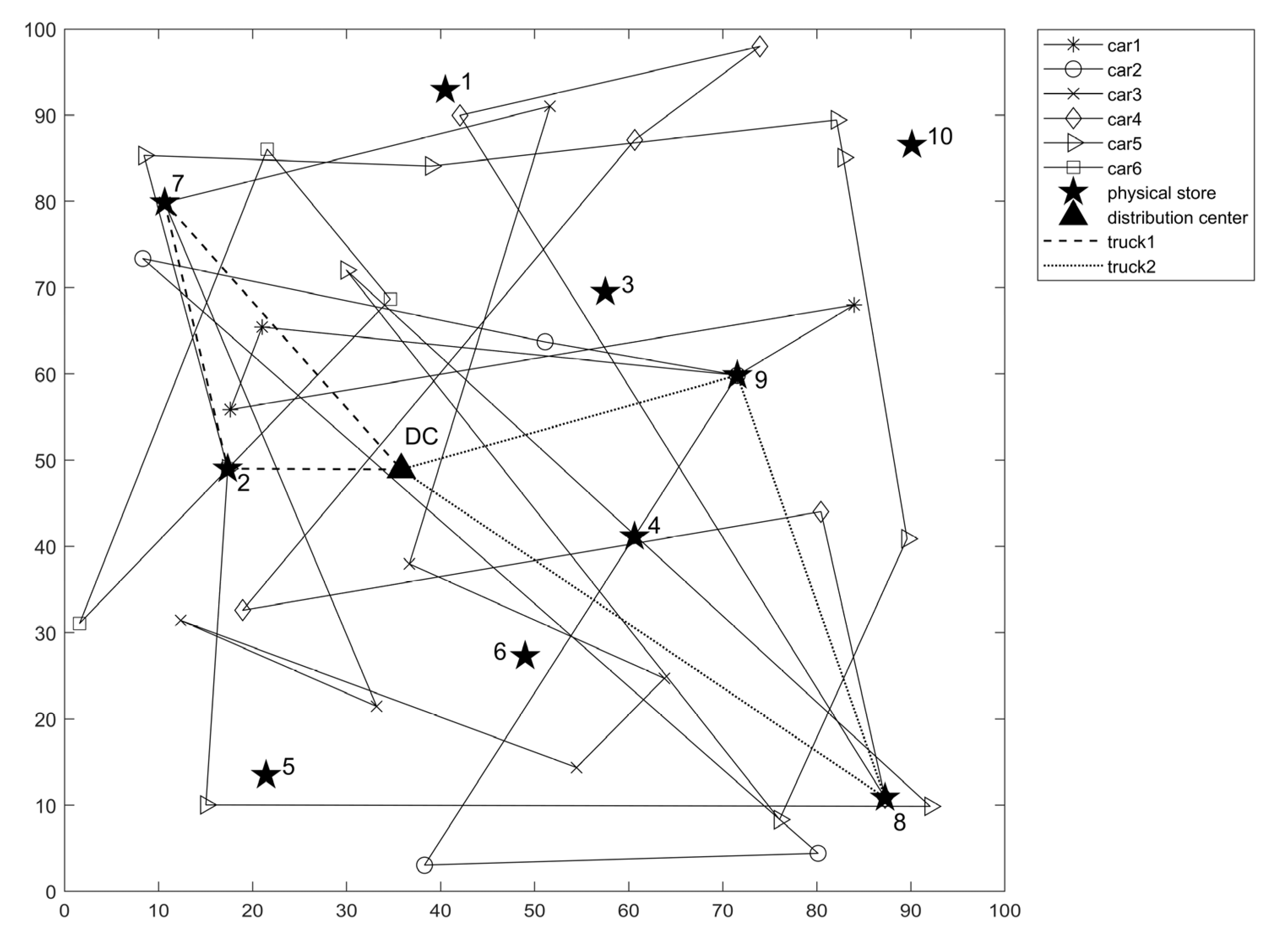
Using the Windows 10 system, we compiled the data in MATLAB R2018a and carried out numerical experiments on a PC with a 1.00 GHz main frequency processor and 8.00 GB of memory. This paper sets the population size as 300 and the maximum number of iterations as 150. The selection rate is set to 0.5. The cross probability adopts the adaptive mechanism = 0.8 and = 0.7. During the mutation operation, we set the dynamic variation probability, a = 0.02, b = 0.1, and y = 10. The above parameters and data were input into the model, and the location results of offline physical stores and distribution routes of vehicles are shown in Figure 3, and the optimization scheme of vehicle distribution routes is shown in Table 7.
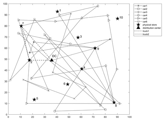
Figure 3.
Schematic diagram of location and distribution route.

Table 7.
Optimization scheme of vehicle distribution route.
It can be seen from Figure 3 that the optimal solution for the location of offline physical stores includes physical stores no. 2, 7, 8, and 9. These four physical stores meet the purchasing demand of customers in the region through the online channel, offline physical channel, and BOPS channel.
Customers will have different selection probabilities for the three purchase channels in the face of different location schemes. Based on the above location scheme, the selection probability of customers at each demand point for the three purchase channels is shown in Table 8.

Table 8.
Selection probability of each demand point for three purchase channels.
It can be seen from Table 4 that total demand of all demand points is 2201.70 kg. Under the above location scheme, it can be seen from Table 8 that the demand of customers in this region is 615.85 kg in the online channel, 736.66 kg in the BOPS channel, and 849.18 kg in the offline physical channel. It can be concluded that after the online retail enterprise expands its offline physical stores to implement the omnichannel retail model, the total amount of products purchased by customers through the BOPS and offline physical channels accounts for about 72.03% of the total demand and that consumers have chosen diversified purchase channels.
4.2. Sensitivity Analysis
The customer’s choice behavior is mainly reflected by the customer’s choice probability of the three purchase channels. In addition to the fact that the location scheme of physical stores affects the pickup distance when customers choose the BOPS channel and the distance to physical store when customers choose the physical channel, thus affecting the customer’s choice behavior, the service level of the physical store, the shopping time, the freight, and return rate of customers choosing the online channel also affect customers’ choice behavior. The shopping time is the customer’s estimate of the time they can spend in a physical store, and enterprises cannot intervene. The freight borne by customers choosing the online channel is a fixed value set by the enterprise, which can be adjusted by the enterprise. Enterprises can also adopt measures such as improving product quality and optimizing online services to reduce the return rate of the online channel. In addition, the service level of physical stores can be improved through staff training and other methods. Therefore, this paper explores the impact of freight, return rate, and service level of physical stores on enterprise costs and customer choice behavior and proposes measures to reduce the enterprise cost of physical store locations.
4.2.1. The Effect of Freight on Total Enterprise Cost and Customer Choice Behavior
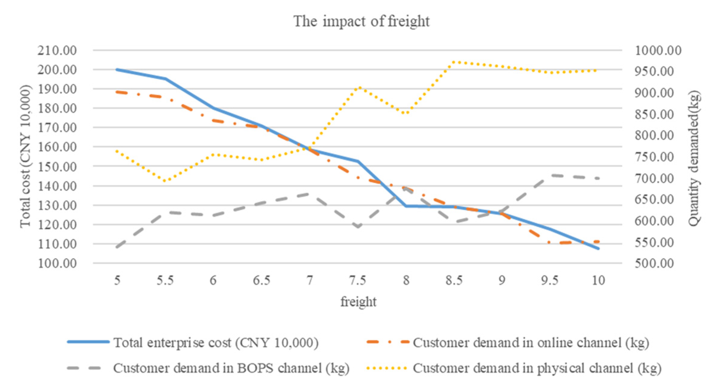
Freight is set to increase from CNY 5 to CNY 10 with a step length of CNY 0.5. Figure 4 shows the results of solving the total enterprise cost and customer demand in the three purchase channels at each freight level.
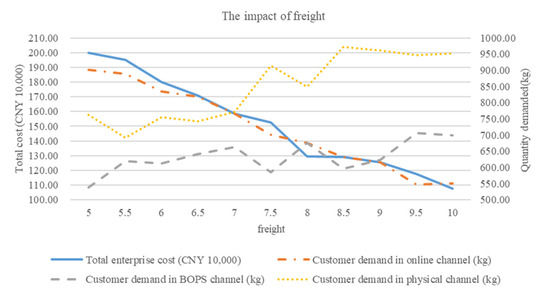
Figure 4.
Freight sensitivity analysis.
As can be seen from Figure 4, with the increase in freight level, the total enterprise cost tends to decline, and customer demand in the online channel gradually decreases, while customer demand in the BOPS channel and offline physical channel generally shows an upward trend. The lower the demand for the online channel, the lower the logistics and distribution cost of the enterprise, and the lower the penalty cost of return, thus reducing the total enterprise cost. It can be concluded that the higher the freight level set by the enterprise, the more customers’ demands in the online channel will be transferred to the BOPS channel and the offline physical channel, which is conducive to reducing the total enterprise cost.
4.2.2. The Effect of Return Rate on Total Enterprise Cost and Customer Choice Behavior
Assuming that the average return rate of each demand point is the same, we set the average return rate of a demand point to increase from 0 to 0.3 in steps of 0.05. Figure 5 shows the results of solving the total enterprise cost and customer demand in the three purchase channels at each level of return rate.
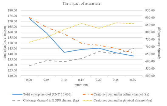
Figure 5.
Sensitivity analysis of return rate.
As can be seen from Figure 5, the higher the return rate of the online channel and the lower customer demand in the online channel, the more necessary it is for new retail enterprises to expand offline physical stores, and the lower the total enterprise cost. It can be concluded that when the return rate of the online channel is high, it is beneficial for an enterprise to expand offline physical stores, and the higher the return rate, the lower the total enterprise cost.
4.2.3. The Effect of the Service Level of Physical Stores on Total Enterprise Cost and Customer Choice Behavior
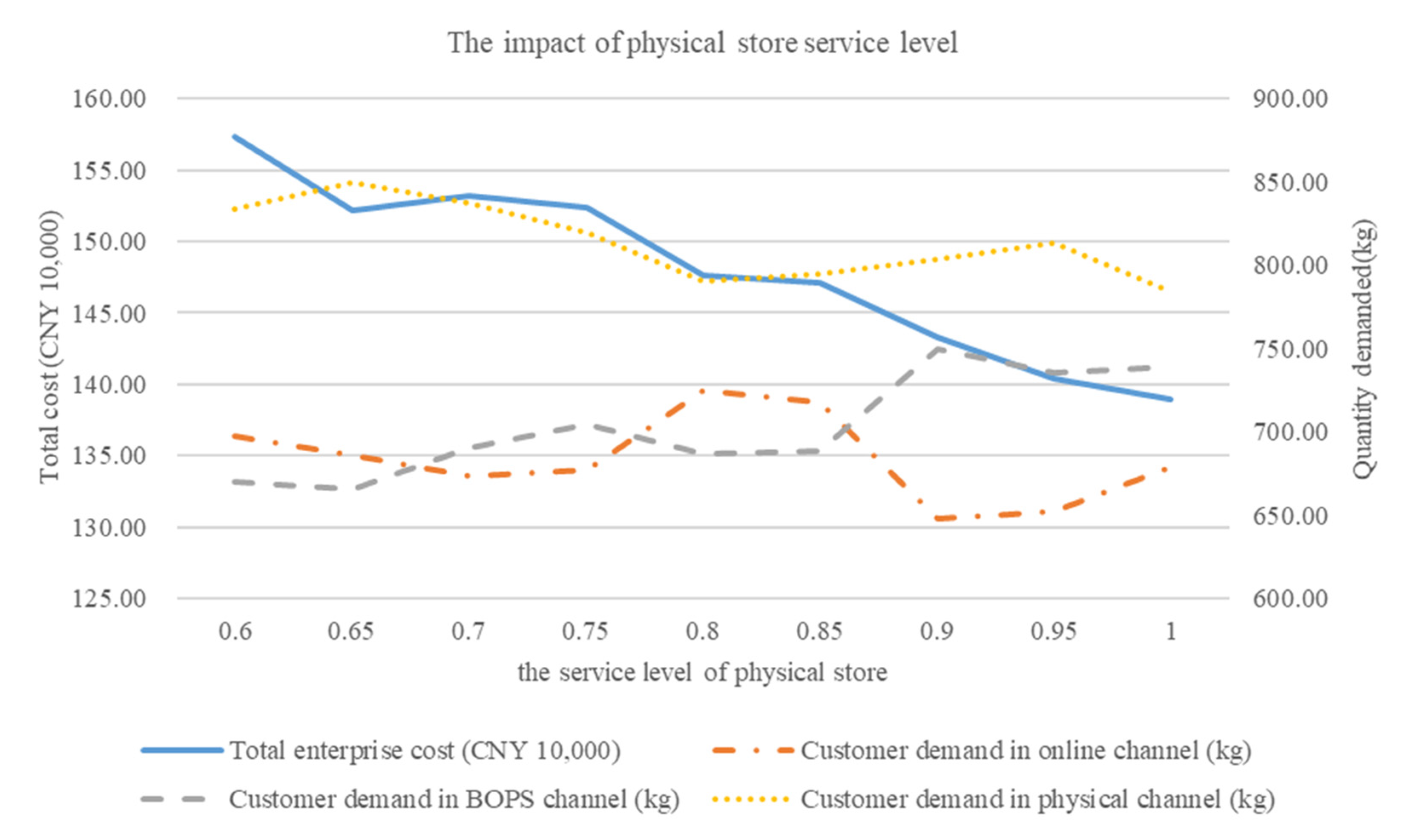
Assuming that the service level of all physical stores is the same, we set the service level of physical stores to increase from 0.6 to 1 in steps of 0.05. Figure 6 shows the results of solving the total enterprise cost and customer demand in the three purchase channels at each service level of physical store.
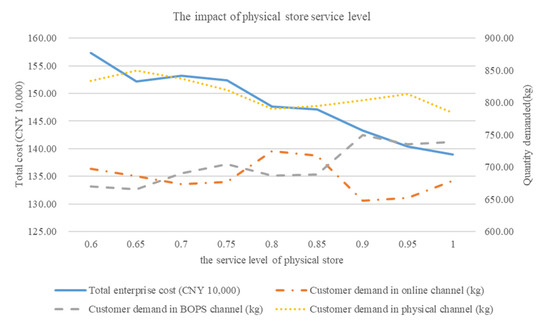
Figure 6.
Sensitivity analysis of physical store service level.
As can be seen from Figure 6, with the improvement of the physical store service level, customer demand in the BOPS channel generally shows an upward trend, while the total enterprise cost generally shows a downward trend, and customer demand in the physical channel always remains the highest. It can be concluded that improving the service level of a physical store can attract more customers to purchase products through the BOPS channel, which is conducive to reducing the total enterprise cost.
4.3. Algorithm Validity Analysis
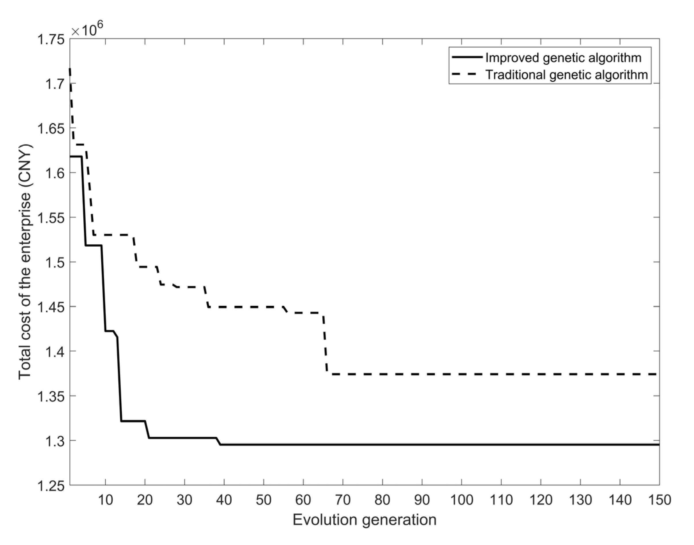
The traditional genetic algorithm is used to solve the model, and the comparison of the algorithm convergence effect is shown in Figure 7. The two algorithms are used to solve the model 10 times each, and the performance indexes of the two algorithms are statistically compared as shown in Table 9.

Figure 7.
Comparison diagram of algorithm convergence.

Table 9.
Comparison of algorithm solution result.
Figure 7 shows that the improved genetic algorithm has a faster convergence speed and higher optimization efficiency. It can be seen from Table 9 that the optimal total cost and average total cost obtained by the improved genetic algorithm are low, the standard deviation of the solution results is small, and the average running time is also significantly reduced. Therefore, the improved genetic algorithm used in this paper is effective and can be used to solve such problems.
5. Conclusions
This paper studies the location problem of offline physical stores of online retail enterprises that plan to implement the BOPS omnichannel retail model and integrates customers’ channel choice behavior into the physical store location process. Considering the construction cost of physical stores, vehicle transportation cost, and penalty cost of customer return, an optimization model of physical store location aiming at minimizing the total cost of the enterprise is constructed. In the model solving stage, we improve the traditional genetic algorithm in the selection mode of chromosomes and determination of crossover and variation probability and improve the efficiency of the algorithm. Finally, an example is calculated to obtain the physical store location scheme considering customer choice behavior and the vehicle scheduling scheme under a two-level distribution network composed of distribution center, physical store, and demand point, which verifies the effectiveness of the model and algorithm. The results of numerical and example analysis show that: after the online retail enterprise expands offline physical stores to implement the omnichannel retail model, the total amount of products purchased by customers through the BOPS and offline physical channels accounts for about 72.03% of the total demand; online retail enterprises can reduce the total cost of physical store location by improving the freight level and the service level of physical stores; the higher the return rate of the online channel, the more necessary it is for online retailers to expand physical stores, and the lower the total cost of physical store location. Based on the research results of this paper, we provide some management suggestions for the operation decision of online retail enterprises in the process of expanding offline physical stores to implement the new retail model.
- (1)
- Enterprises should pay more attention to freight level and enhance offline business capabilities
This study shows that the freight level and the service level of offline physical stores have an important impact on the total enterprise cost. Although the higher freight level and service level of offline physical stores can reduce enterprise cost of physical store location, excessive freight will reduce customers’ demand in the online channel, resulting in poor shopping experience, and bring operational pressure to offline physical stores. Therefore, enterprises should set reasonable freight levels according to their own business conditions and enhance offline business capabilities.
- (2)
- Enterprises should take measures to reduce return rate
The higher the return rate of the online channel, the more necessary it is for online retail enterprises to expand offline physical stores. On the one hand, the higher online return rate reduces customers’ shopping experience; on the other hand, the recovery and disposal of returned products will also increase the enterprise’s cost.
This paper faced certain limitations, and further research remains necessary in the future. First of all, this study considers that under the relatively saturated online shopping market, there is no product shortage problem in any channel of new retail enterprises. In fact, there may be situations where products are out of stock in one channel, leading consumers to choose other channels. In addition, this paper does not consider the existence of competitive enterprises. In future research, we can take the situation of product shortage in channels into consideration in the consumer choice model and also consider consumer choice behavior and the location of physical stores in the presence of competitive enterprises. For the characterization of consumer choice behavior, other alternative models can be further verified in the future.
Author Contributions
Conceptualization, P.W.; methodology, P.W. and J.Z.; software, J.Z.; validation, P.W., J.Z. and Y.L.; formal analysis, P.W. and J.Z.; investigation, P.W., J.Z., Y.L. and X.J.; resources, P.W.; data curation, P.W., J.Z. and X.J.; writing—original draft preparation, J.Z.; writing—review and editing, P.W. and J.Z.; visualization, J.Z.; supervision, P.W.; project administration, P.W. All authors have read and agreed to the published version of the manuscript.
Funding
This research received no external funding.
Institutional Review Board Statement
Not applicable.
Informed Consent Statement
Not applicable.
Data Availability Statement
The data presented in this study are available in the article.
Conflicts of Interest
The authors declare no conflict of interest.
References
- Difrancesco, R.M.; van Schilt, I.M.; Winkenbach, M. Optimal in-store fulfillment policies for online orders in an omni-channel retail environment. Eur. J. Oper. Res. 2021, 293, 1058–1076. [Google Scholar] [CrossRef]
- Song, Y.; Fan, T.; Tang, Y.; Xu, C. Omni-channel strategies for fresh produce with extra losses in-store. Transp. Res. Part E Logist. Transp. Rev. 2021, 148, 102243. [Google Scholar] [CrossRef]
- Saha, K.; Bhattacharya, S. ‘Buy online and pick up in-store’: Implications for the store inventor. Eur. J. Oper. Res. 2021, 294, 906–921. [Google Scholar] [CrossRef]
- Zhang, A.; Ren, J.; Guan, Z.; Farooq, U. Decision and Coordination in the Dual-Channel Supply Chain Considering the Risk-Averse and Customer Returns. J. Math. Financ. 2021, 11, 48–83. [Google Scholar] [CrossRef]
- Esmaeili, N.; Teimoury, E.; Pourmohammadi, F. A scenario-based optimization model for planning and redesigning the sale and after-sales services closed-loop supply chain. RAIRO-Oper. Res. 2021, 55, S2859–S2877. [Google Scholar] [CrossRef]
- Pangarkar, A.; Arora, V.; Shukla, Y. Exploring phygital omnichannel luxury retailing for immersive customer experience: The role of rapport and social engagement. J. Retail. Consum. Serv. 2022, 68, 103001. [Google Scholar] [CrossRef]
- Momen, S.; Torabi, S.A. Omni-channel retailing: A data-driven distributionally robust approach for integrated fulfillment services under competition with traditional and online retailers. Comput. Ind. Eng. 2021, 157, 107353. [Google Scholar] [CrossRef]
- Adivar, B.; Hüseyinoğlu, I.Y.; Christopher, M. A quantitative performance management framework for assessing omnichannel retail supply chains. J. Retail. Consum. Serv. 2019, 48, 257–269. [Google Scholar] [CrossRef]
- Gallino, S.; Moreno, A. Integration of Online and Offline Channels in Retail: The Impact of Sharing Reliable Inventory Availability Information. Manag. Sci. 2014, 60, 1434–1451. [Google Scholar] [CrossRef]
- Huang, J.; Shi, X. Solving the location problem of front distribution center for omni-channel retailing. Complex Intell. Syst. 2021, in press. [CrossRef]
- Xu, N.; Huang, Y.-F.; Weng, M.-W.; Do, M.-H. New Retailing Problem for an Integrated Food Supply Chain in the Baking Industry. Appl. Sci. 2021, 11, 946. [Google Scholar] [CrossRef]
- Gao, F.; Su, X. Omnichannel Retail Operations with Buy-Online-and-Pick-up-in-Store. Manag. Sci. 2017, 63, 2478–2492. [Google Scholar] [CrossRef]
- Fan, X.; Tian, L.; Wang, C.; Wang, S. Optimal service decisions in an omni-channel with buy-online-and-pick-up-in-store. J. Oper. Res. Soc. 2020, 73, 794–810. [Google Scholar] [CrossRef]
- Radhi, M.; Zhang, G. Optimal cross-channel return policy in dual-channel retailing systems. Int. J. Prod. Econ. 2019, 210, 184–198. [Google Scholar] [CrossRef]
- Pichka, K.; Alwan, L.C.; Yue, X. Fulfillment and pricing optimization for omni-channel retailers considering shipment of in-store demand. Transp. Res. Part E Logist. Transp. Rev. 2022, 167, 102912. [Google Scholar] [CrossRef]
- Paul, J.; Agatz, N.; Savelsbergh, M. Optimizing Omni-Channel Fulfillment with Store Transfers. Transp. Res. Part B Methodol. 2019, 129, 381–396. [Google Scholar] [CrossRef]
- Bayram, A.; Cesaret, B. Order Fulfillment Policies for Ship-from-Store Implementation in Omni-Channel Retailing. Eur. J. Oper. Res. 2020, 294, 987–1002. [Google Scholar] [CrossRef]
- Wang, M.; Wang, Y.; Liu, W.; Ma, Y.; Xiang, L.; Yang, Y.; Li, X. How to achieve a win–win scenario between cost and customer satisfaction for cold chain logistics? Phys. A Stat. Mech. Its Appl. 2021, 566, 125637. [Google Scholar] [CrossRef]
- Wang, Y.; Assogba, K.; Liu, Y.; Ma, X.; Xu, M.; Wang, Y. Two-echelon location-routing optimization with time windows based on customer clustering. Expert Syst. Appl. 2018, 104, 244–260. [Google Scholar] [CrossRef]
- Dou, S.; Liu, G.; Yang, Y. A New Hybrid Algorithm for Cold Chain Logistics Distribution Center Location Problem. IEEE Access 2020, 8, 88769–88776. [Google Scholar] [CrossRef]
- Zhang, S.; Chen, N.; She, N.; Li, K. Location optimization of a competitive distribution center for urban cold chain logistics in terms of low-carbon emissions. Comput. Ind. Eng. 2021, 154, 107120. [Google Scholar] [CrossRef]
- Li, X.; Zhou, K. Multi-objective cold chain logistic distribution center location based on carbon emission. Environ. Sci. Pollut. Res. 2021, 28, 32396–32404. [Google Scholar] [CrossRef] [PubMed]
- Alamatsaz, K.; Ahmadi, A.; Al-E-Hashem, S.M.J.M. A multiobjective model for the green capacitated location-routing problem considering drivers’ satisfaction and time window with uncertain demand. Environ. Sci. Pollut. Res. 2022, 29, 5052–5071. [Google Scholar] [CrossRef] [PubMed]
- Ouyang, J.; Fan, H.; Wang, L.; Yang, M.; Ma, Y. Site Selection Improvement of Retailers Based on Spatial Competition Strategy and a Double-Channel Convolutional Neural Network. ISPRS Int. J. Geo-Inf. 2020, 9, 357. [Google Scholar] [CrossRef]
- Agrebi, M.; Abed, M. Decision-making from multiple uncertain experts: Case of distribution center location selection. Soft Comput. 2021, 25, 4525–4544. [Google Scholar] [CrossRef]
- Fathi, M.; Khakifirooz, M.; Diabat, A.; Chen, H. An integrated queuing-stochastic optimization hybrid Genetic Algorithm for a location-inventory supply chain network. Int. J. Prod. Econ. 2021, 237, 108139. [Google Scholar] [CrossRef]
- Liu, Z.; Wu, Z.; Ji, Y.; Qu, S.; Raza, H. Two-stage distributionally robust mixed-integer optimization model for three-level location-allocation problems under uncertain environment. Phys. A Stat. Mech. Its Appl. 2021, 572, 125872. [Google Scholar] [CrossRef]
- Marianov, V.; Eiselt, H.; Lüer-Villagra, A. Effects of multipurpose shopping trips on retail store location in a duopoly. Eur. J. Oper. Res. 2018, 269, 782–792. [Google Scholar] [CrossRef]
- Zhang, H.; Feng, H.; Wang, H. Two-Stage Optimization Model of Agricultural Product Distribution in Remote Rural Areas. IEEE Access 2020, 8, 213928–213949. [Google Scholar] [CrossRef]
- Yu, V.F.; Jodiawan, P.; Hou, M.-L.; Gunawan, A. Design of a two-echelon freight distribution system in last-mile logistics considering covering locations and occasional drivers. Transp. Res. Part E Logist. Transp. Rev. 2021, 154, 102461. [Google Scholar] [CrossRef]
- Yang, J.; Guo, F.; Zhang, M. Optimal planning of swapping/charging station network with customer satisfaction. Transp. Res. Part E Logist. Transp. Rev. 2017, 103, 174–197. [Google Scholar] [CrossRef]
- Xu, X.; Jackson, J.E. Investigating the Influential Factors of Return Channel Loyalty in Omni-Channel Retailing. Int. J. Prod. Econ. 2019, 216, 118–132. [Google Scholar] [CrossRef]
- Marianov, V.; Ríos, M.; Icaza, M.J. Facility location for market capture when users rank facilities by shorter travel and waiting times. Eur. J. Oper. Res. 2007, 191, 32–44. [Google Scholar] [CrossRef]
- Zhang, Y.; Berman, O.; Verter, V. The impact of client choice on preventive healthcare facility network design. OR Spectr. 2012, 34, 349–370. [Google Scholar] [CrossRef]
- Haase, K.; Müller, S. Insights into clients’ choice in preventive health care facility location planning. OR Spectr. 2015, 37, 273–291. [Google Scholar] [CrossRef]
- Al-Salih, W.; Esztergár-Kiss, D. Linking Mode Choice with Travel Behavior by Using Logit Model Based on Utility Function. Sustainability 2021, 13, 4332. [Google Scholar] [CrossRef]
- Kucukyazici, B.; Zhang, Y.; Ardestani-Jaafari, A.; Song, L. Incorporating Patient Preferences in the Design and Operation of Cancer Screening Facility Networks. Eur. J. Oper. Res. 2020, 287, 616–632. [Google Scholar] [CrossRef]
- Krohn, R.; Müller, S.; Haase, K. Preventive healthcare facility location planning with quality-conscious clients. OR Spectr. 2021, 43, 59–87. [Google Scholar] [CrossRef]
- Haase, K.; Müller, S. A comparison of linear reformulations for multinomial logit choice probabilities in facility location models. Eur. J. Oper. Res. 2014, 232, 689–691. [Google Scholar] [CrossRef]
- Chen, Y.; Han, P.; Zeng, Q. Multi-objective location problem of pick-up point considering the impact of home delivery. Comput. Integr. Manuf. Syst. 2016, 22, 2679–2690. (In Chinese) [Google Scholar] [CrossRef]
- Chen, G.; Fu, J.; He, M. Emergency Shelter Location Problem Considering Residents’ Choice Behavior. Oper. Res. Manag. Sci. 2019, 28, 6–14. (In Chinese) [Google Scholar] [CrossRef]
Publisher’s Note: MDPI stays neutral with regard to jurisdictional claims in published maps and institutional affiliations. |
© 2022 by the authors. Licensee MDPI, Basel, Switzerland. This article is an open access article distributed under the terms and conditions of the Creative Commons Attribution (CC BY) license (https://creativecommons.org/licenses/by/4.0/).

